1. Introduction
Channel estimation is a fundamental issue to be addressed in wireless communication systems since its accuracy has a significant impact on the recovery of the received signals as well as the management of interference suppression and wireless resource allocation and other tasks [
1]. According to whether prior information is used, the channel estimation methods can be divided into three categories, which are the blind estimation method, the pilot-based estimation method, and the semi-blind estimation method, respectively. In particular, blind estimation methods acquire channel state information (CSI) from the structure and statistics of the received signals, while pilot-based estimation methods allocate a part of wireless resource to transmit known signals to obtain CSI. To enable high precision channel estimation performance, the latter has been widely used [
2].
For a future beyond 5G and 6G communication systems, it is more challenging to acquire channel estimation results with high accuracy since many higher mobility and denser-connection scenarios will appear [
3]. As introduced in [
4], the accuracy of channel estimation can benefit from the increase in the number of pilots. To support the estimation accuracy to satisfy the requirements of service in a complex channel environment, typical conventional channel estimation methods, such as the least square (LS) estimator and the minimum mean square error (MMSE) estimator, have to add many more pilots. However, it declines the spectral efficiency of communication systems due to more wireless resources being allocated to transmit pilot signals. In addition, both methods have their own shortcomings [
5]. Specifically, the LS estimator cannot be used to estimate data channels directly, while the MMSE estimator needs to know the statistical characteristics of both pilot and data channels in advance and consumes extra computational resources to perform the matrix inversion operation.
To overcome these bottlenecks, some deep learning-based channel estimation methods have been developed. According to whether the conventional channel estimation method is combined, the main idea of these methods can be classified in the following two categories. On the one side, there are some works focusing on designing neural networks as the denoising module embedded into existing conventional estimation methods. In [
6], the authors employed two convolutional neural networks (CNNs) connected sequentially to denoise and smooth the channel matrix obtained by using conventional interpolation methods. A scheme that denoises the received signals based on CNN model at first and then estimates channel coefficients by using conventional estimation methods was proposed in [
7]. On the other side, some studies are dedicated to learning the correlation between pilot channels and data channels by using neural networks. In [
8], a CNN model was trained to learn the time–frequency correlation so that the complete channel matrix can be obtained by feeding pilot channels into the model. Moreover, Ref. [
9] designed a CNN model to learn the time–frequency–spatial correlation in massive multiple-input–multiple-output (MIMO) systems. However, it is worth pointing out that although the performance can be improved significantly by comparing with conventional methods, most of the designed structure of neural networks is very dependent on the specific pilot configuration. It means that the model needs to be retrained once the pilot configuration changes, which cannot provide adaptive deployment.
As a newly emerging neural network structure, GAN has shown powerful performance in generating synthetic samples following real data distribution [
10], which has been applied in many aspects, including image generation [
11], image restoration [
12], dataset extension [
13], communication networks [
14] and others. In the wireless communication domain, the GAN-based channel modeling in complex channel environment has attracted a lot of attention. In particular, Ref. [
15] has studied the feasibility of using the conditional GAN model to replace the modeling channel transfer function. Therefore, a more precise parametric backpropagation can be guaranteed during the training process of an end-to-end communication system. By employing the federated learning framework [
16,
17], a distributed conditional GAN framework was proposed in [
18] to enable multiple users to train a global model collaboratively. In terms of the channel estimation problem, some GAN-based schemes have been proposed to enhance estimation accuracy and reduce pilot overhead. In [
19,
20], GAN was employed to learn the distribution of channel correlation matrix in vehicular millimeter wave systems and frequency division duplex massive MIMO systems, respectively. Moreover, Ref. [
21] provided a scheme aiming to learn the gradient of any point in high-dimensional channel space, in which any channel to be estimated can be recovered by following the learned gradient direction. However, consuming a large amount of storage resource is the shortcoming of this scheme. In addition, Ref. [
22] proposed a virtual pilot generation-based scheme, where GAN is used to learn the correlation between pilot signals. By combining real pilots with generated virtual pilots, the channel estimation accuracy can be improved without extra cost of wireless resource. Furthermore, GAN has been used to learn the correlation between elements of channel matrix directly in [
23]. With the aid of compressed sensing, the channel can be estimated without a significant loss of accuracy when more than a half of the number of pilots is reduced.
Although the above GAN-based works have explored the ability of GAN to learn the distribution of multiorder statistics for wireless channels in depth, they mainly focus on low-speed mobile users and neglect to be compatible with high-speed mobile users. In this paper, a novel two-stage channel estimation method based on GAN is proposed to guarantee flexible channel estimation under any pilot configuration and the performance evaluation is extended into the medium- and high-speed mobile scenario for OFDM systems. In particular, a GAN model is designed to learn the correlation between elements of the channel matrix in the first stage. During the second stage, a channel recovery method is given to achieve channel estimation via using the pretrained GAN model. In particular, our proposed scheme can estimate data channels directly via the given pilots without generating extra virtual pilots at first and then using the conventional interpolation method as introduced in [
22], which facilitates the efficiency of channel estimation. Moreover, compared with [
23], our proposed scheme does not need to find a measurement matrix that is necessary for compressed sensing. The main contribution of this paper is summarized as follows:
Firstly, a novel GAN-based channel estimation method is proposed, in which the coefficients over all data channels are obtained by matching the coefficients of real channels and generated channels at pilot positions. Meanwhile, the compressed low-dimensional latent variable is obtained simultaneously, which can be used to support the CSI feedback service with a low communication overhead.
Secondly, the simulation results are provided to show the performance gain obtained by using our proposed method. In particular, by comparing with the conventional Wiener filtering interpolation method, our proposed method can improve the accuracy performance by more than 2 dB with a reduction of the number pilots when the signal-to-noise (SNR) is 10 dB. It shows the potential to reduce the pilots overhead drastically. The achieved compression ratio in this experiment is 2.4%.
3. A GAN Based Channel Estimation Scheme
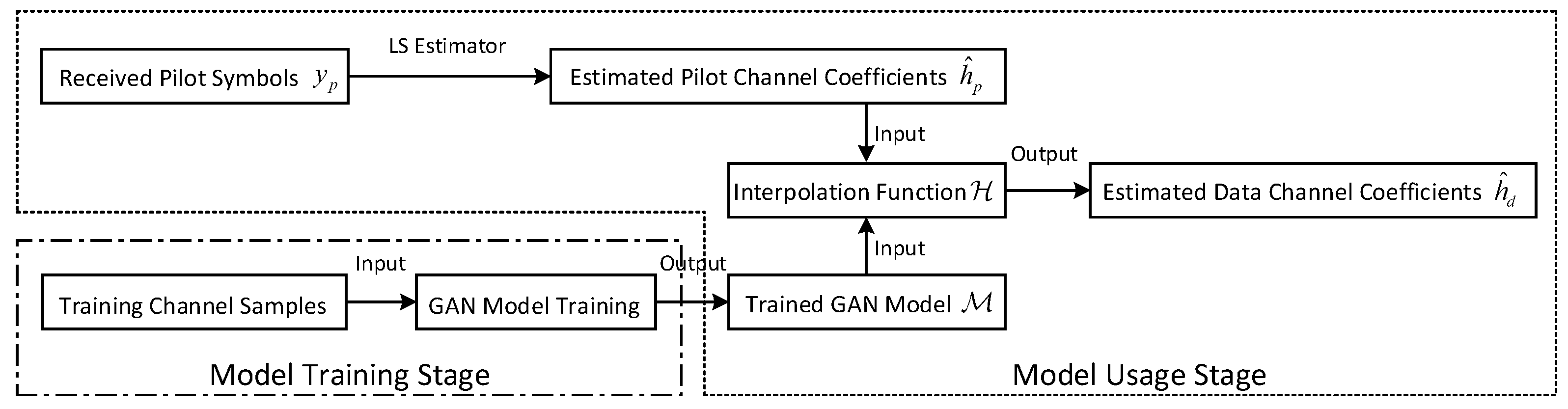
In this section, a novel channel estimation method based on GAN is provided. The pipeline of our proposed channel estimation scheme is illustrated in
Figure 2. As shown in
Figure 2, the procedure contains two stages, which are the model training and model usage stages, respectively. During the model training stage, a designed GAN model is trained to be capable of producing synthetic OFDM channel samples that are similar to the real OFDM channel samples. In particular, the model training stage can be conducted offline or online. For the offline training case, the model can be trained with pre-collected channel samples so that it can be applied directly during communications. In the case of online training, the model is trained with samples collected in the current channel environment, which makes the learned characteristic distribution of channels more in line with the current scenario. Hence, there is a trade-off about deployment latency and synthetic channel samples similarity between offline and online modes. The selection of an appropriate training mode is customized according to different requirements of services. In addition, the joint utilization of both modes is feasible, which can be done by training a preset model offline and fine-tuning it online. During the model usage stage, the already trained GAN model combined with the estimated pilot channel coefficients
is imported into a designed interpolation function
to obtain the data channel coefficients
. The details of these two stages are presented in the following two subsections.
3.1. Model Training Stage: Training A GAN Model to Capture the Distribution of Real Channel
In this subsection, the procedure of generating synthetic channel samples with high similarity to real channel samples by training a GAN model is illustrated in detail. Firstly, the basic concept of GAN is provided as follows.
3.1.1. Basic Framework of GAN
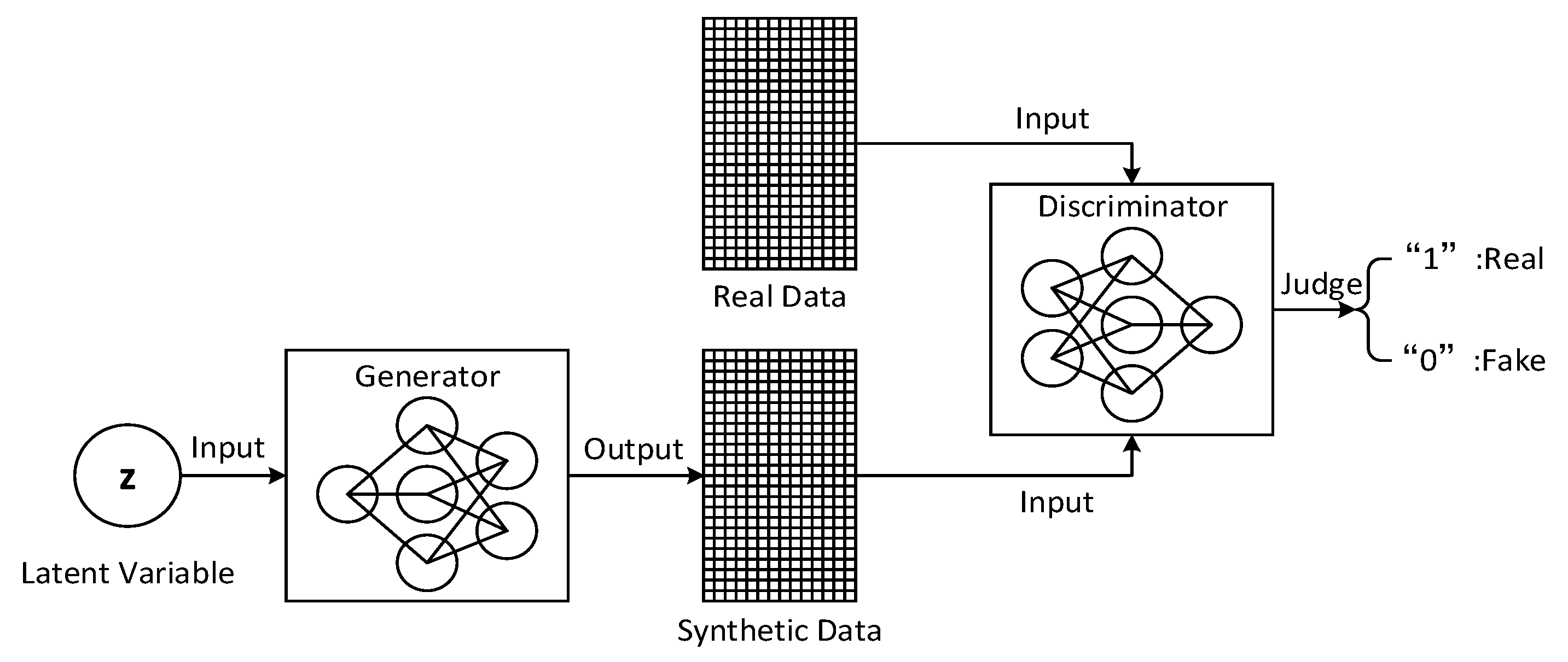
As shown in
Figure 3, the general structure of GAN is depicted. It consists of two independent neural networks, which are named generator
G and discriminator
D [
10], respectively. In particular, the generator aims to learn the mapping relationship from a latent variable
z in low-dimensional space to the real data samples in high-dimensional space. In the ideal case, the trained generator can produce a large variety of different synthetic channel samples that follow the real data distribution. The key goal of discriminator is to distinguish whether the input data come from the real dataset. Generally, to achieve this goal, the output layer of the discriminator network is designed to be a sigmoid function such that a probability value
labeling the input data can be obtained,
. When
approaches 1, it means that the input data sample is most likely to be a real data sample, while when
approaches 0, it means that the input data sample, with high probability, belongs to the synthetic sample set.
Since the generator tries to generate data samples capable of confusing the discriminator while the discriminator aims to distinguish synthetic data samples produced by the generator from the real data samples, the key objectives of the generator and discriminator are in conflict. Therefore, a min-max game problem for training the GAN model can be formulated, which is expressed as [
10]
where
and
denote the parameters of generator and discriminator, respectively,
and
are the output of the generator and discriminator, respectively, and
and
are the probability distribution of the latent variable
z and real dataset, respectively.
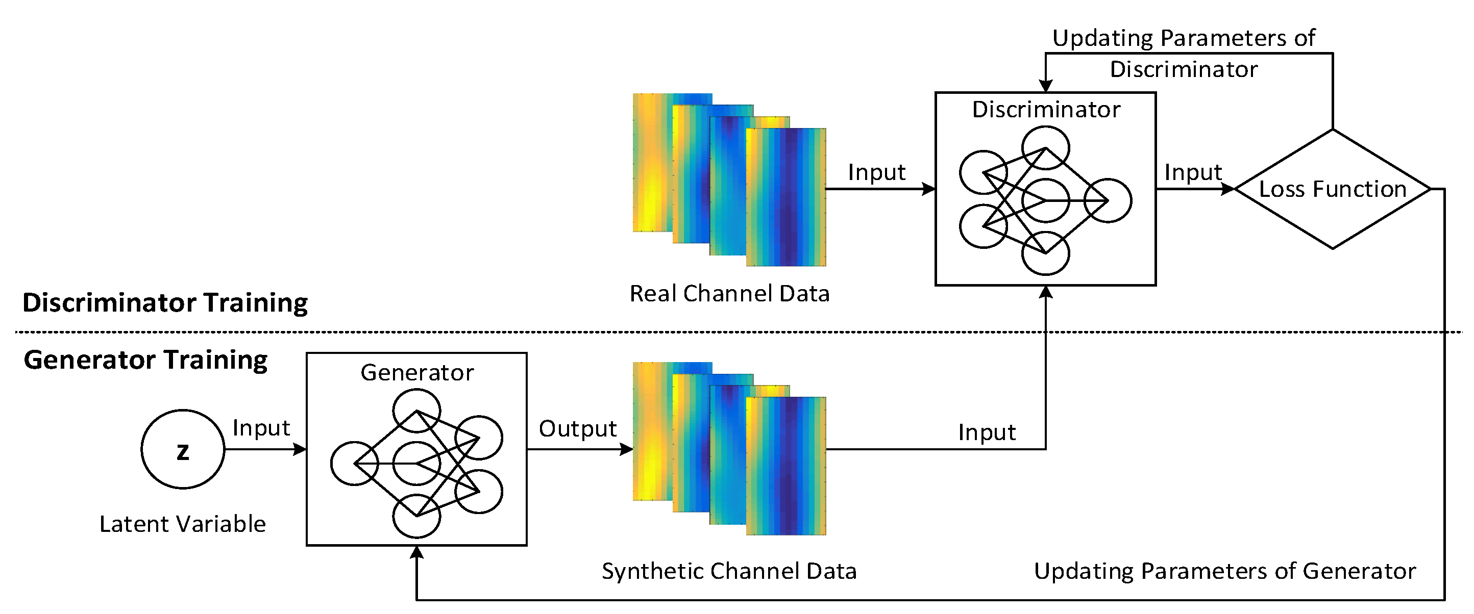
3.1.2. Training Procedure of a GAN Model
The specific procedure of training a GAN model that generates synthetic channel samples is depicted in
Figure 4. As shown in this figure, the training of the generator and discriminator are conducted iteratively. The training procedure can be divided into two cases based on the types of data samples fed into the discriminator. In particular, when real channel data samples are inputted, only the parameters of discriminator need to be updated. The discriminator tries to maximize the output probability
so that every real sample can be identified well, and its training objective can be expressed as
Moreover, when synthetic channel data samples generated by the generator are fed into the discriminator, both the parameters of the generator and discriminator are ready to be updated. Specifically, in terms of the discriminator, its training objective is to minimize the output probability
so that the synthetic samples can be distinguished, which is written as
As for the generator, its training objective is to maximize the output probability
so that the produced synthetic samples can deceive the discriminator to regard themselves as real samples, which is expressed as
Based on the training objectives
in (
7),
in (
8) and
in (
9), the procedure of training a GAN model to generate synthetic channel samples is summarized in Algorithm 1. In Algorithm 1, the generator is trained once when the parameters of the discriminator have finished
R times updates, which is of benefit for balancing the performance between the generator and discriminator during the training procedure and avoiding the mode collapse issue [
27]. The parameters can be updated via using gradient descent methods. In addition, the widely used cross entropy function is usually selected as the loss function for training the GAN model. After the GAN model is converged, stable synthetic channel samples can be generated.
| Algorithm 1 GAN-based synthetic channel samples generation. |
Initialization:, , the maximum number of iterations K, the ratio of training rounds between the discriminator and generator r, batch size , learning rate , the form of loss function , and the convergence threshold . Repeat: For k-th iterations, Sample real channel samples; Generate synthetic channel samples by feeding sampled latent variables z independently into the generator; Feed real samples and synthetic samples into the discriminator, then calculate the loss function with respect to real samples as , and calculate the loss function with respect to synthetic samples as ; Update by following ; Ifk mod r , do generator training: Generate another synthetic channel samples and feed into discriminator; Calculate the loss function ; Update by following .
Termination: When or and . Output: Trained discriminator with parameters and generator with parameters .
|
3.2. Model Usage Stage: Using Generator Model to Achieve Data Channel Estimation
In this subsection, the trained GAN model is used to estimate the data channels with the pilot channels known. The channel recovery problem is similar to the image completion problem in the computer vision domain [
12]. This problem can be solved based on the premise condition that any channel images following the real data distribution can be generated if the generator is well trained. Since there is a one-to-one correspondence between the latent variable and the channel matrix, there is potential to find the target entire channel with the partial pilot channels information known by adjusting the latent variable
z. Thus, the original channel recovery problem
given by (
5) can be transformed into the search problem of an optimal latent variable
, which is expressed as
where
.
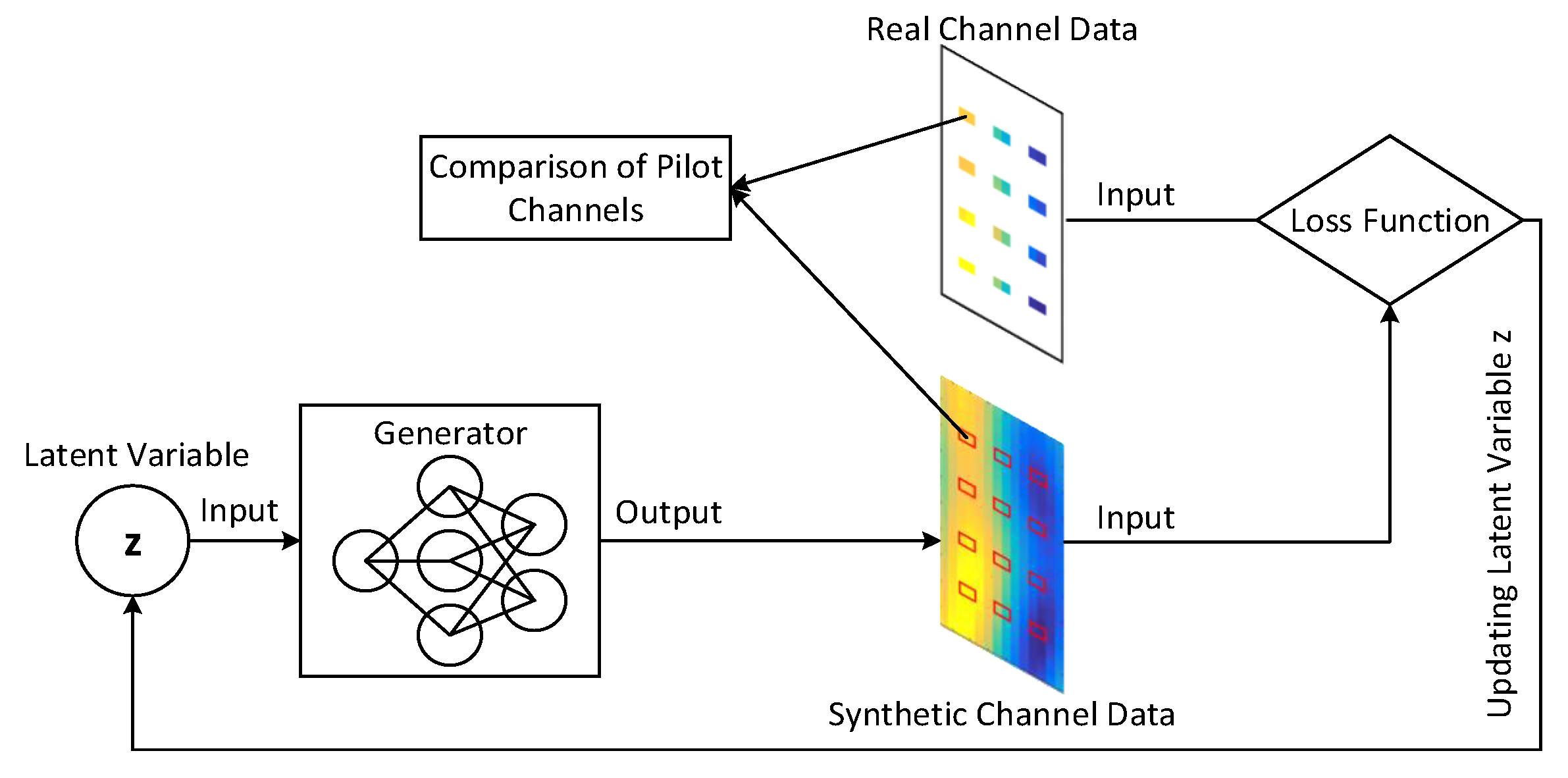
The procedure of recovering data channels to solve
is presented in
Figure 5. Note that only the generator model is involved in channel estimation. During the searching process, the trained generator is used without parameter modification. The entire process can be regarded as the interpolation function
defined in (
5). As shown in
Figure 5, the comparison between the real channels and the generated channels over all pilot positions is conducted to determine the gap between each other. Afterward, the value of latent variable
z can be updated by using gradient descent methods, which makes the new output generated channels at pilot positions closer to the real ones. Once the gap is minimized, an optimal latent variable
that reconstructs the pilot channels faithfully can be found. Hence, the channels over all data positions will be recovered well due to the learned strong correlations among elements. The corresponding algorithm is provided in Algorithm 2.
| Algorithm 2 Generator based Channel Estimation. |
Initialization: Trained generator model , latent variable , learning rate , the form of loss function , the maximum number of iterations L and the convergence threshold . Input: The position indicator of pilot channels , , . Obtain the estimated channel coefficients of all pilot elements based on ( 3); Repeat: For l-th iterations, Generate a synthetic channel sample with latent variable ; Calculate the gap between and over all pilot channels; Feed into the loss function ; Update by following .
Termination: When or . Output: The recovered entire channel matrix .
|
In Algorithm 2, the optional loss function has a wide range, including -norm and -norm and others. When the updating process of latent variable z is terminated, the final version of recovered entire channel matrix with both pilot and data channels can be obtained. Note that the proposed algorithm is available for supporting the implement of any pilot configuration without retraining the neural network since there is no reliance on pilot information during the training process of the GAN model. Therefore, the proposed scheme does not require additional training cost if the pilot configuration changes, which is beneficial for flexible deployment.
4. Simulation Settings and Results
In this section, simulation results are provided to show the performance gain of our proposed GAN-based channel estimation scheme. In particular, the OFDM channel dataset containing
samples is generated by following the TDL-C channel model [
28], which characterizes the Rayleigh fading channel environment in the urban macrocell scenario under the non-line of sight (NLOS) condition. The ratio of the training samples to the total samples is set as
. Power normalization is operated for all samples. The number of subcarriers and symbols within each OFDM block are set as
and
, respectively. The carrier frequency is set as
GHz, and the bandwidth of each subcarrier is set as
kHz. The time interval of an OFDM block is set as
ms. To avoid the inter symbol interference, the cyclic prefix accounting for
of the symbol length is added to the front of each symbol. In addition, to ensure that the maximal propagation delay is not larger than the duration of cyclic prefix, the root mean square (RMS) delay spread is considered to be set as
ns. Moreover, the scenario that the terminal user moving with high speed is also considered, in which two speed cases are simulated, which are
km/h and
km/h, respectively.
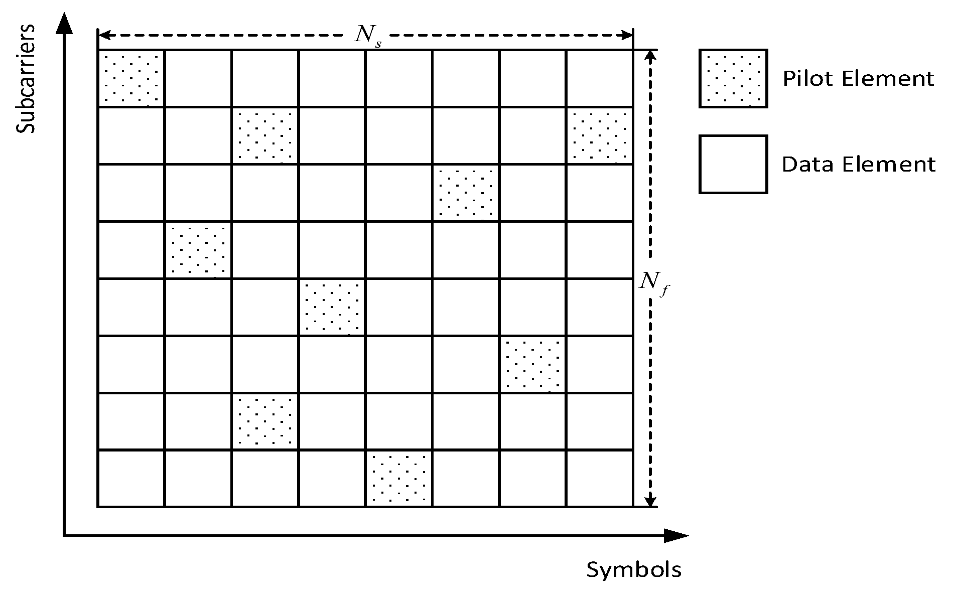
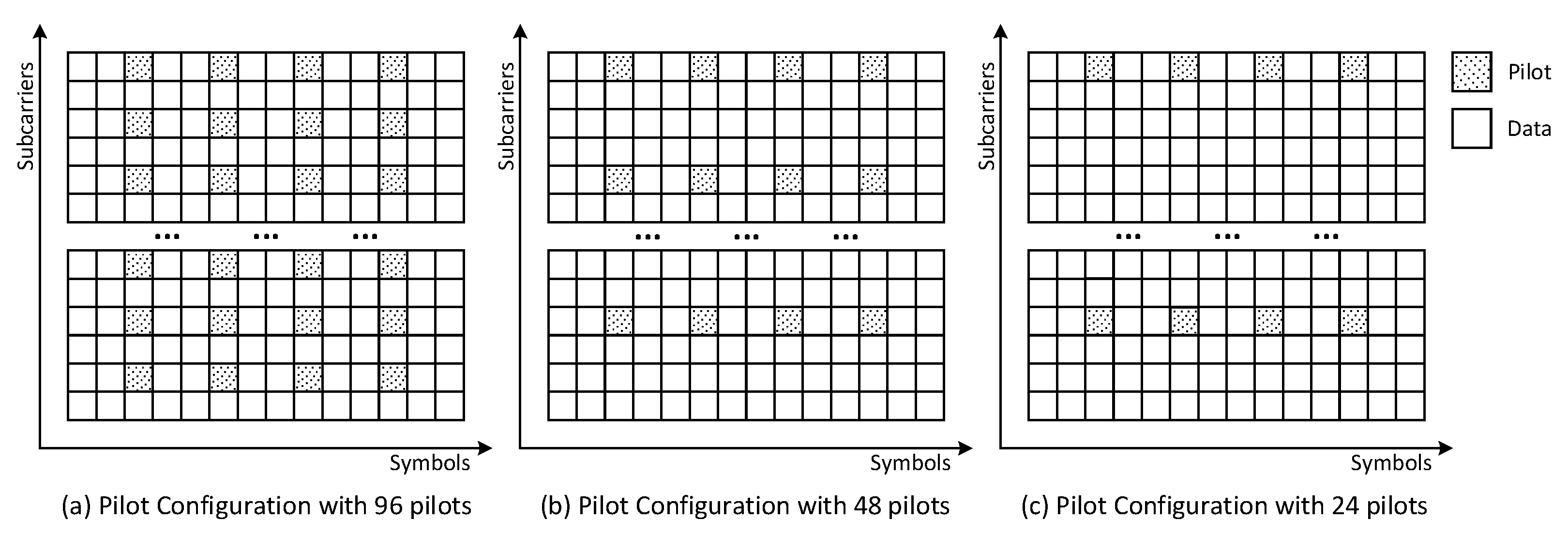
As shown in
Figure 6, three types of pilot configurations with different numbers of pilots are considered in the evaluation of the channel estimation performance. To reduce the cost of pilots and ensure the efficiency of data transmission, the maximum number of pilot elements is limited to 96. In particular, the pilot positions are designed on the same columns for all three configuration schemes, which are the 3, 6, 9, and 12-th columns. The aim of configuring the sparse pilot pattern is to capture the fast-changing trend of the channel environment. The only difference between these three schemes is the row positions of pilots. Specifically, in the cases of pilot configurations (a), (b) and (c), the pilots are inserted every two rows, every four rows, and every eight rows, respectively.
To evaluate the accuracy of the channel estimation, the performance metric needs to be determined at first. The normalized mean square error (NMSE) that has also been used in [
6,
7,
23] is selected as the metric in this paper, and its definition can be expressed as
where
n denotes the index of test sample.
Next, the architecture of the GAN model used in this experiment is shown in detail. The subsequent subsection gives the simulation results.
4.1. GAN Model Architecture
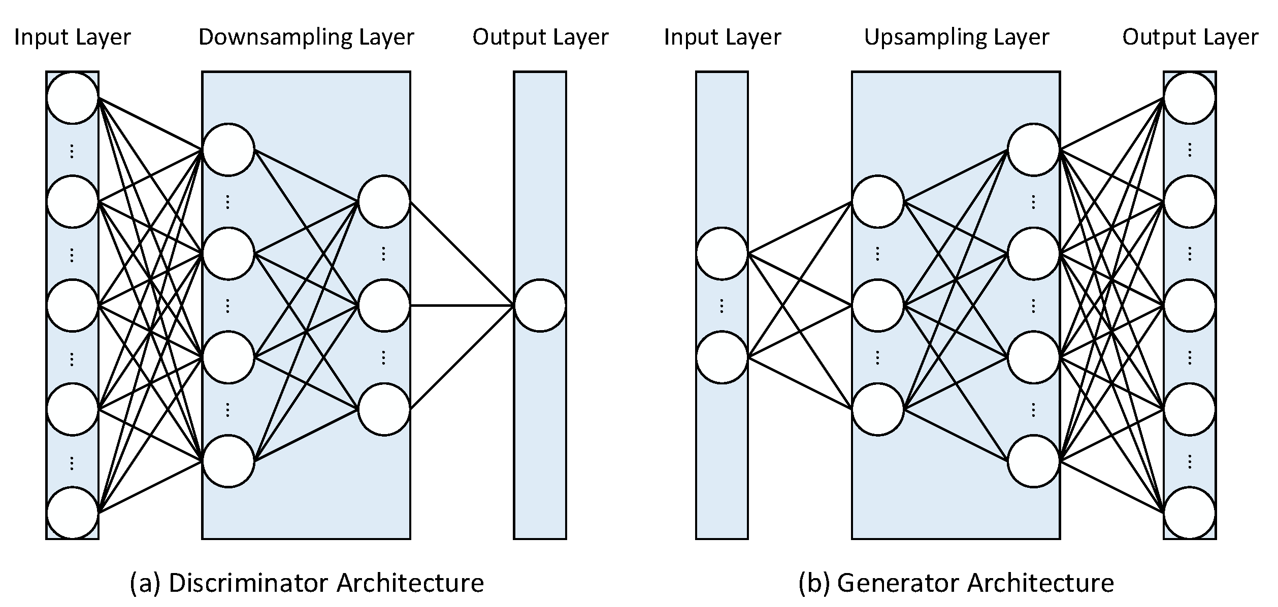
The architectures of discriminator and generator are illustrated in
Figure 7a,b, respectively. As shown in this figure, both models are designed as fully connected networks with five linear layers. In the case of the discriminator, the input channel sample is flattened into a vector from the original matrix. Considering that the coefficient of the channel is with a complex form, an efficient way to handle this is to split it into the real and imaginary parts. In this experiment, the real part and the imaginary part are treated as two different samples. Hence, the input layer is still designed with
neurons. The hidden layer consists of three downsampling layers, which contain 512, 256 and 64 neurons, respectively. The first four layers are each followed by a LeakyReLU active function and a LayerNorm normalized function. Finally, the output layer contains only one neuron followed by a sigmoid function, which outputs a probability
to judge the authenticity of the input samples.
In the case of the generator, the input latent variable
z is designed as a standard Gaussian vector with
dimensions. To evaluate the compression degree of the original channel matrix by the generator, the compression ratio is defined as the ratio of the dimension of
z to the dimension of
h, which is expressed as
Based on (
12), the compression ratio in this experiment is
. It means that the proposed method can also be used for CSI feedback services to reduce the communication overhead drastically. The hidden layer consists of three upsampling layers that are symmetric to the downsampling layers of the discriminator. Similar active and normalized functions are inserted between the first four layers. In the end, the output layer contains 672 neurons connected with the Tanh activation function.
Other hyperparameters are summarized as follows. The ratio of training rounds between discriminator and generator is set as
. To generate synthetic channel samples with high quality, it is recommended to train the GAN model with a large number of epoches [
23,
29]. Thus, the parameters of the GAN model are updated by using the RMSprop optimizer with learning rate
for up to 1000 epoches. The loss function
is set as the binary cross entropy function. In addition, the loss function
in Algorithm 2 is set as the
-norm function.
4.2. Simulation Results
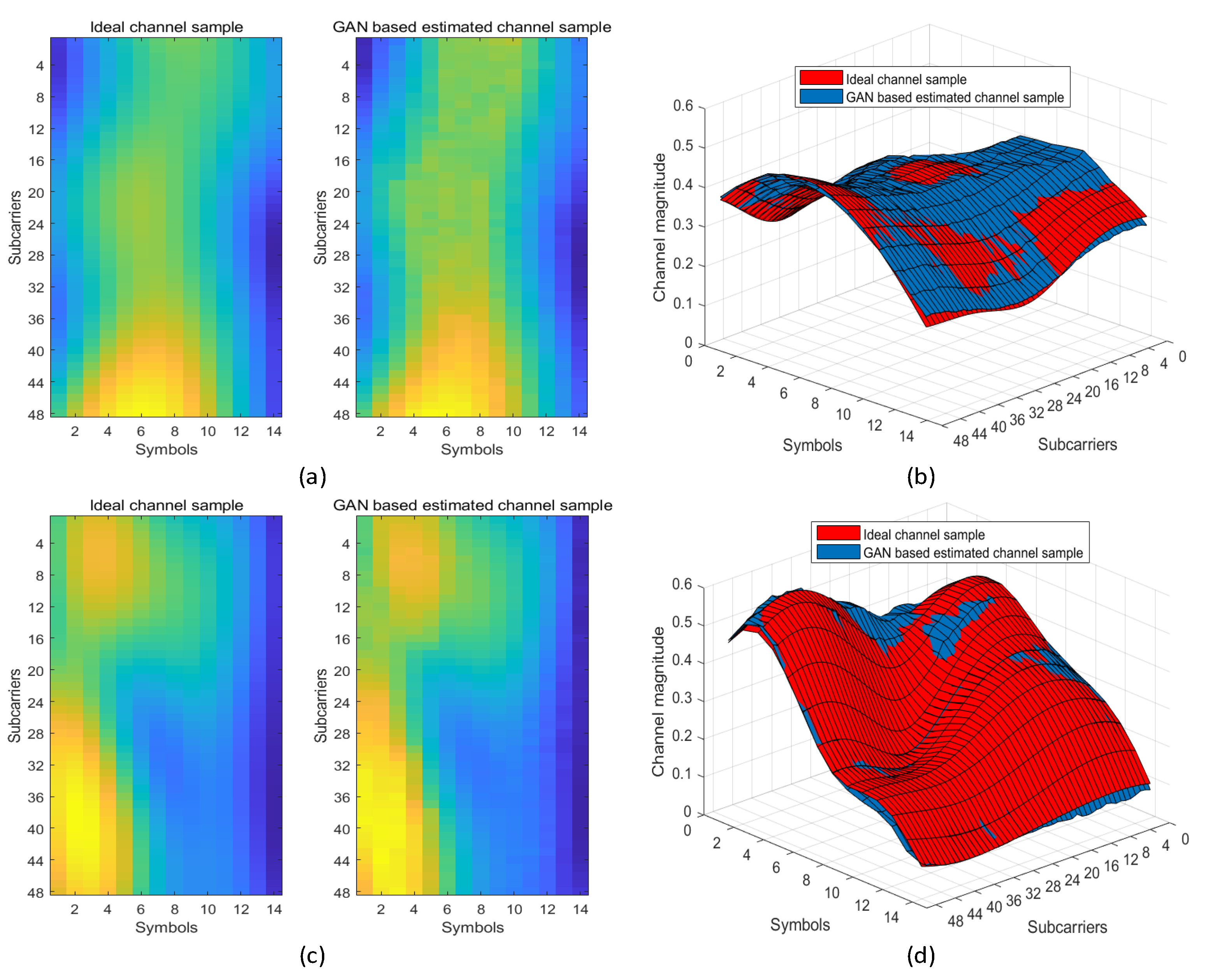
In
Figure 8, the comparisons between the magnitude of channel coefficients estimated by our proposed GAN based method and those of the ground truth channel samples in both medium- and high-speed mobile scenarios are provided. In particular, the pilot configuration setting follows the scheme shown in
Figure 6a. As shown in this figure, the channel changes more dramatically in the high-speed scenario than that in the medium-speed scenario. The channel variation trends of the estimated results in both scenarios coincide well with those of the ground truth results from both the two-dimensional and three-dimensional perspectives. Moreover,
Figure 8b,d show that the estimated results are only with a limited error, which verifies the feasibility of our proposed method.
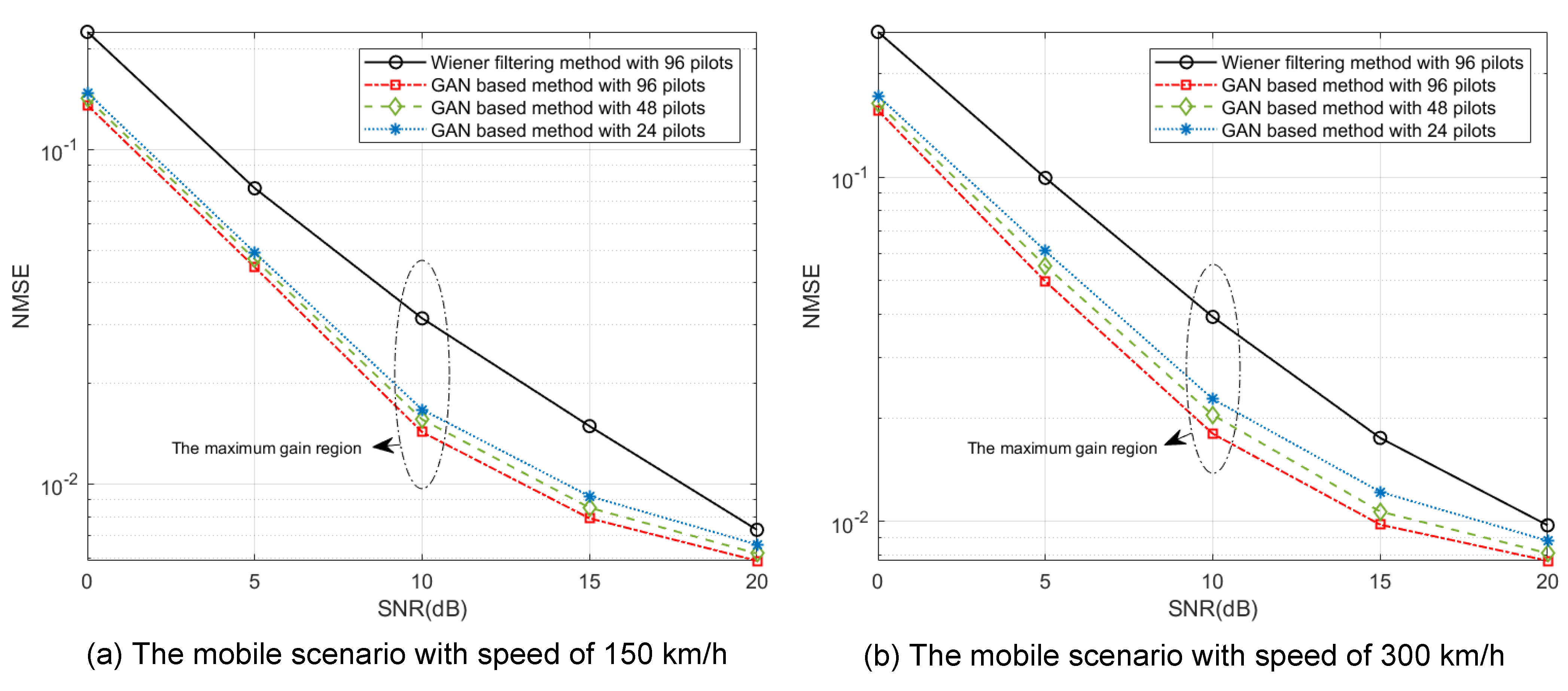
As shown in
Figure 9, the evaluation for the accuracy performance of our proposed GAN-based channel estimation method is provided, where two mobile scenarios with speeds of 150 km/h and 300 km/h are considered in
Figure 9a,b, respectively. In addition, the pilot configuration settings are given in
Figure 6. In particular, the widely used conventional Wiener filtering interpolation method [
30], a method that can achieve the MMSE criteria when SNR is high enough, is selected as the benchmark. The estimated data channels after Wiener filtering can be expressed as
where
denotes the filtering matrix, which is pre-estimated in the link-level simulation platform. In the mobile scenario with speed of 150 km/h shown in
Figure 9a, compared with the conventional method, the GAN-based methods always outperform, even with a fewer number of pilots. However, when SNR is low, neither the conventional method nor the proposed GAN-based method can achieve good performance due to the existence of non-negligible error for the channel coefficients at pilot positions estimated by the LS method. The maximum gain can be obtained when SNR is 10 dB. Specifically, the performance gain is
dB,
dB and
dB when the number of pilot is 96, 48 and 24, respectively. It shows that the proposed method can reduce the pilot overhead by
with only
dB performance loss. As the SNR increases, the performance of the proposed method will converge to a stable level due to the learning ability being limited by the experimental model structure. By re-designing a more complicated network structure, the error will converge to a smaller value.
Moreover, in the mobile scenario with a speed of 300 km/h shown in
Figure 9b, the performance curves follow a similar trend with those in the mobile scenario with a speed of 150 km/h. In particular, the achieved accuracy performance is lower than that in
Figure 9a due to the more variable channel environment. The maximum gain also appears in the case that SNR is 10 dB, where the performance gains under 96, 48 and 24 pilots conditions are
dB,
dB and
dB, respectively. It shows that the estimation error of the proposed method increases 1 dB when
pilots are removed. It can be observed that as the number of pilots decreases, the performance gain decays faster in the high speed scenario than that in the medium-speed scenario; as a result, the accurate acquisition of channel correlation in a complex channel environment needs sufficient pilots.
5. Conclusions
In this paper, we studied the feasibility of using the GAN model to address the channel estimation problem in the scenarios where the channel varies dramatically toward future 6G communication systems. Specifically, the entire estimation process contains two stages, which are the model training stage and the model usage stage. In the model training stage, a pre-designed GAN model is used to learn the channel distribution. In the model usage stage, based on the learned correlation between elements in channel matrix, the data channel coefficients are recovered via matching the generated pilot channel coefficients by the trained GAN model and real pilot channel coefficients by the LS method. Hence, the proposed GAN-based scheme can support the channel estimation for any pilot configuration. Simulation results show that our proposed method can improve the estimation accuracy with a large reduction in the pilots overhead in both medium- and high-speed mobile scenarios. Meanwhile, the corresponding channel matrix is compressed to a low dimension, which is also useful for dramatically reducing the feedback overhead in the CSI feedback service. For future works, the pilot channels’ denoised scheme can be considered to combine with the proposed method to further improve the channel estimation performance, especially in the low SNR cases.


