Study of Local Fatigue Methods (TCD, N-SIF, and ESED) on Notches and Defects Related to Numerical Efficiency

Featured Application

Feasible engineering methods to assess the fatigue strength of irregularly shaped planar imperfections and pore networks by linear–elastic numerical analysis.

Abstract

The fatigue strength of structural components is strongly affected by notches and imperfections. Both can be treated similarly, as local notch fatigue strength methods can also be applied to interior defects. Even though Murakami’s √area approach is commonly used in the threshold-based fatigue design of single imperfections, advanced concepts such as the Theory of Critical Distances (TCD), Notch Stress Intensity Factors (N-SIF), or Elastic Strain Energy Density (ESED) methods provide additional insight into the local fatigue strength distribution of irregularly shaped defects under varying uniaxial load vectors. The latter methods are based on the evaluation of the elastic stress field in the vicinity of the notch for each single load vector. Thus, this work provides numerically efficient methods to assess the local fatigue strength by means of TCD, N-SIF, and ESED, targeting the minimization of the required load case count, optimization of stress field evaluation data points, and utilization of multi-processing. Furthermore, the Peak Stress Method (PSM) is adapted for large opening angles, as in the case of globular defects. In detail, two numerical strategies are devised and comprehensively evaluated, either using a sub-case-based stress evaluation of the defect vicinity with an unchanged mesh pattern and varying load vector on the exterior model region with optimized load angle stepping or by the invocation of stress and strain tensor transformation equations to derive load angle-dependent result superposition while leaving the initial mesh unaltered. Both methods provide numerically efficient fatigue post-processing, as the mesh in the evaluated defect region is retained for varying load vectors. The key functions of the fatigue strength assessment, such as the evaluation of appropriate planar notch radius and determination of notch opening angle for the discretized imperfections, are presented. Although the presented numerical methods apply to planar simulation studies, the basic methodology can be easily expanded toward spatial fatigue assessment.

1. Introduction

Local fatigue approaches, such as the notch stress concept, were originally developed for welded joints, thereby featuring a fictitious notch rounding including a microstructural support effect [1,2,3,4]. Recent contributions also provide strain-based approaches to assess the fatigue life until crack initiation in arbitrarily notched parts [5,6]. If large-scale yielding needs to be considered, fatigue crack growth based on cyclic plastic strain is applicable instead [7].

Conversely, the stress field at the weld toe—or weld root—region can be assessed as a pointed V-notch, including the scale effect [8]. In various components, exterior notches and interior defects can be treated similarly [9,10,11,12,13]. The stress distribution in the vicinity of the V-notch is representative of the fatigue limit. In notched component design, the fatigue stress limit is often evaluated at a characteristic distance from the notch tip, according to the Theory of Critical Distances (TCD) [14,15]. As the stress distribution in sharp V-notched parts is singular, the dimensioning by notch stress intensity factors (N-SIF) depends on the opening angle. Thus, a unified fatigue assessment for different notch angles is possible, either by means of the peak stress method (PSM) as a rapid fatigue assessment tool [16,17] or by averaging the elastic strain energy density (ESED) within a certain control volume [18,19,20,21,22].

In summary, for linear–elastic stress field evaluation of a notched (or imperfected) component under uniaxial loading, the TCD, N-SIF, and ESED methods can all be used. Global approaches, such as Murakami’s method [23,24,25] for single imperfections or the extension towards extreme value statistics [26,27,28,29], account for fatigue strength by evaluation of the projected defect area of the representative defect but do not take the effect of orientation on the global load vector into account.

The basic principles of the TCD, N-SIF, and ESED methods, as local fatigue design approaches, are briefly reviewed in the following.

First, the Theory of Critical Distances (TCD) [14,15] is a local fatigue assessment tool requiring only the evaluation of the stress field at a dedicated point away from the notch tip [30,31]. In the case of the Point Method, the stress is evaluated at a distance of $a_0/2$ from the notch tip. The El Haddad–Smith–Topper parameter $a_0$ [32] is material-dependent and indicates its supporting effect. The evaluated fatigue strength was originally threshold-based [33,34], while a recent extension toward finite life fatigue assessment has been introduced in [35,36,37], and exemplified for macroscopic imperfections in [38].

In the case of notch stress intensity factor (N-SIF)-based design, the fatigue limit is determined by the stress field distribution of V-notches. The stress field singularity at sharp notches $r\to 0$ can be described using William’s eigenvalues ${\mathsf{\lambda }}_1,{\mathsf{\lambda }}_2$ [39] for varying opening angles. If a polar coordinate system originating from the notch tip is aligned to the notch bisector, the N-SIF value quantifies the asymptotic stress distribution in the close neighborhood, as exemplified for Mode I in Equation (1). The numerical N-SIF assessment of sharp V-notches is evaluated accordingly in this study.

$$K_I^V=\sqrt{2 \pi }\underset{r\to 0}{\lim }\left[{\left({\sigma }_{\theta }\right)}_{\theta =0}{r}^{1-{\lambda }_1}\right]$$

(1)

A link between the exact value of the notch stress intensity factor $K_I^V$ of V-notches with varying opening angles and maximum elastic peak stress ${\sigma }_{peak}$ at the notch tip has been presented in [40], as well as analytically proven. A non-dimensional ratio $K_{FE,I}^{*}$ (Equation (2)) exists between the notch stress intensity factor $K_I^V$, the peak stress ${\sigma }_{peak}$, and the edge length of the linear quadrilateral finite element $d$ at the notch tip, powered by $1-{\lambda }_1$ as the notch angle contribution. The non-dimensional ratio is illustrated for Mode I, evaluated as $K_{FE,I}^{*}$ = 1.38.

$$K_{FE,I}^{*}=\frac{K_I^V}{{\sigma }_{peak} d^{1-{\lambda }_1}}$$

(2)

It should be noted that the peak stress method includes the rapid fatigue assessment of the N-SIF for varying V-notch opening angles between $0°\le 2\alpha \le 135°$ and linear element types [41]. As the finite element simulation requires only the linear–elastic material properties, the non-dimensional ratio $K_{FE,I}^{*}$ is solver-independent [42].

For multi-axial stress conditions, an equivalent peak stress can be calculated if synchronous stress contributions are given [43]. In the case of non-proportional loads, a local biaxiality ratio selects the proper peak stress method-based design scatter band [44].

To apply the N-SIF approach to blunt cracks, the stress field is calculated based on the sharp notch stress field by adding a supplementary term [45,46] and linked to the maximum principal stress at the notch tip. Evaluating the blunt V-notch stress intensity factor away from the notch tip, as generalized N-SIF, has been recommended in [47] and, accordingly, is applied in this study. The evaluated $K_{\rho ,I}^V$ is averaged across a distance of approximately $r=r_0\to r_0+0.4\rho$ from the notch tip. The parameters ${\mu }_1$ and ${\tilde{\omega }}_1$ depend on the notch opening angle $2\alpha$, whereas $r_0$ depends also on the notch radius $\rho$. Mode I loading is detailed in Equation (3), for reference.

$$K_{\rho ,I}^V=\sqrt{2 \pi }{r}^{1-{\lambda }_1}\frac{{\left({\sigma }_{\theta }\right)}_{\theta =0}}{1+{\tilde{\omega }}_1{\left(\frac{r}{r_0}\right)}^{{\mu }_1-{\lambda }_1}}$$

(3)

Elastic strain energy density (ESED) fatigue design is based on the distribution of the stress and strain fields away from the notch tip within a certain control volume. An energy-based fatigue assessment for sharp V-notches under fatigue loading has been presented in [48]. Under the plane strain condition, Equation (4) depicts the dependence of the critical radius $R_c$—and, therefore, the control volume $\mathsf{\Omega }$—on the material threshold of the stress intensity factor range $\mathsf{\Delta }{K}_{th}$ for long cracks and the endurance stress range $\mathsf{\Delta }{\sigma }_0$.

$$R_c=\frac{\left(1+\mathsf{\nu }\right)\left(5-8\mathsf{\nu }\right)}{4\mathsf{\pi }}{\left(\frac{\mathsf{\Delta }{K}_{th}}{{\mathsf{\Delta }\mathsf{\sigma }}_0}\right)}^2$$

(4)

The El Haddad–Smith–Topper parameter $a_0$ [32] is linked to the critical control radius $R_c$ by Poisson’s ratio $\mathsf{\nu }$ and the appropriate stress state. For $\mathsf{\nu }=0.3$, this equates to $R_c=0.845a_0$ for plane strain and to $R_c=1.025a_0$ for plane stress condition. The plane strain state leads to a reduced control volume, thus favouring a conservative fatigue assessment. Under the plane strain condition, the range of the elastic strain energy density, averaged over the control volume $\mathsf{\Omega }$, can be expressed analytically for sharp notches [49]. The parameter $e_1$ depends on the notch opening angle $2\alpha$ and Poisson’s ratio $\nu$. The radius of the control volume is given by the critical radius $R_c$, which originates in the case of sharp notches at the notch tip. Equation (5) depicts only the contribution of Mode I.

$$\mathsf{\Delta }W=\frac{e_1}{E}{\left[\frac{\mathsf{\Delta }{K}_I^V}{R_c^{1-{\lambda }_1}}\right]}^2$$

(5)

The total elastic strain energy density can be related to the notch stress intensity factor, or in terms of the peak stress [50,51,52]. To account for the scale effect under non-linear material behavior, either plastic notch stress intensity factors [53,54] or total strain energy density fatigue design utilizing both the elastic and plastic energy fractions [55,56,57] can be exploited. The cumulative value of the strain energy density can be linked to the number of cycles to failure [58,59]. Thus, the crack initiation sites can be well-identified by strain energy density evaluation within a notched component [60,61,62]. Multi-axial loads can be taken into account by evaluating the energy density in critical planes [63,64].

The aim of this work is to provide a methodology to set up numerical methods, realizable using commercially available finite element codes and user-defined scripting, which support the efficient evaluation of irregularly shaped defects under varying uniaxial tensile load vectors. At a glance, numerically efficient fatigue post-processing tools for planar meshes featuring a notched component are based on maintaining an unchanged mesh pattern within the notch vicinity, even for varying load vectors. Thus, local evaluation methods, such as interpolation of nodal stresses at TCD-specific points or calculation of element fractions within a certain control volume for ESED fatigue assessment, may be computed only once for several load cases. As only planar studies are considered in this work, the uniaxial tension load vector is rotated along half of the defect circumference. The applied load angle stepping, as well as the mesh-seed of the defect-afflicted model, determine the overall computation time. Key parameters affecting the calculated fatigue strength distribution, such as the global mesh-seed or control radius $R_c$, are also identified and discussed.

In general, if the chosen local fatigue concept is based only on the stress field, such as the case in the TCD or N-SIF fatigue assessment methods, stress transformation of the basic load steps for varying uniaxial load vectors is recommended in post-processing. Thereby, the nodal stress results are not simulated by means of finite element studies for each load vector but computed through post-processing transformation of the stress or strain tensor.

If the fatigue design is to be based on ESED values, a sub-case-based approach is preferable, which allows for improved accuracy. This implies the splitting of the input model into a defect area with a circular border, which is glued to the rectangular bounding box. The latter bounding box component is rotated for each uniaxial load vector, but the interior part of the model is kept unchanged. Although an increased number of load case simulation runs is needed, the post-processing stage is simplified, as the additional transformations are omitted.

Finally, the overall wall-time demand of the scripts dealing with curvature calculation, stress path evaluation, and control volume computation can be significantly improved through the utilization of multi-processing computation modules.

2. Methodology

As the TCD, N-SIF, and ESED approaches are already well-established in the field of notch fatigue design, the first step toward numerically efficient methods for arbitrarily shaped imperfections is to set up a basic simulation study of a V-notched specimen and validate the results using published data. A sharp notched flat plate under tension loading, with parameters of the double lateral V-shaped notch, in accordance with the peak stress study in [40,41], was used as the basic geometry. The link to the elastic strain energy within the control volume has been detailed in [49]. Blunt V-notch studies relating to N-SIF and ESED assessment have been previously examined in [19]. In summary, the comprehensive analytical equations presented in [19,49] were used to validate the basic V-notched simulation study depicted in Figure 1. A flat plate with a double lateral V-notch was simulated and geometrically defined according to the plate width $W$, notch depth $a$, opening angle $2\alpha$, and (in the case of the blunt notch) radius $\rho$. The depicted linear–elastic simulation features plane-strain condition and unified tension loading in the gross-section of the plate.

The linear–elastic material properties were defined according to Young’s modulus $E=206 \mathrm{GPa}$ and Poisson’s ratio $\nu =0.3$. Moreover, the critical radius was set to $R_c=0.19 \mathrm{mm}$, implying a value of $a_0=0.225 \mathrm{mm}$, in accordance with the data published in [57]. This material dataset was used consistently in all following studies.

The discretized geometry of any arbitrarily shaped planar defect must be assessed for each point along the defect circumference, which can be either treated as sharp V-notch, assuming a small notch root radius (see Equation (1)), or as blunt V-notch for larger root radii, implying a stress evaluation ahead of the notch tip (Equation (3)). The stress field in the vicinity of sharp and blunt V-notches was evaluated as a basic reference example, as detailed in

Table 1. N-SIF and ESED results of a basic study on double-notched V-plate (W = 10 mm, a = 1 mm, 2α = 90°) in plane strain formulation.

Notch Tip Radius	${\mathit{K}}_{\mathit{I}}^{\mathit{V}}{}^{ 1}$	${\mathit{K}}_{\mathit{I}}^{\mathit{V}}{}^{ 2}$	$\mathbf{\Delta }{\mathit{W}}^{ 1}$	$\mathbf{\Delta }{\mathit{W}}^{ 2}$
$\rho =0 \mathrm{mm}$	$2.295{ \mathrm{MPamm}}^{0.456}$	$2.316{ \mathrm{MPamm}}^{0.456}$	$1.681\times {10}^{-5} \mathrm{mJ}/{\mathrm{mm}}^3$	$1.698\times {10}^{-5} \mathrm{mJ}/{\mathrm{mm}}^3$
$\rho =1 \mathrm{mm}$	$2.589{ \mathrm{MPamm}}^{0.456}$	$2.602{ \mathrm{MPamm}}^{0.456}$	$1.282\times {10}^{-5} \mathrm{mJ}/{\mathrm{mm}}^3$	$1.328\times {10}^{-5} \mathrm{mJ}/{\mathrm{mm}}^3$

¹ Simulation results using Ansys^® Build 21.1/Plane183 elements. ² Analytical result using equations given in [49] for sharp and [19] for blunt notches.

. In addition to the numerical results, the published analytical formulae for N-SIF and ESED are included for comparison, based on matching stress paths in the vicinity of the notch tip.

The stress results of the Point Method for the two investigated notches (Figure 1) are given in

Table 2. TCD results of a basic study on double-notched V-plate (W = 10 mm, a = 1 mm, 2α = 90°) in plane strain formulation.

Notch Tip Radius	${\mathit{\sigma }}_{\mathit{\theta }}{\left(\raisebox{1ex}{${\mathit{a}}_0$}\!\left/ \!\raisebox{-1ex}{$2$}\right.\right)}^{ 1}$	${\mathit{\sigma }}_{\mathit{\theta }}{\left(\raisebox{1ex}{${\mathit{a}}_0$}\!\left/ \!\raisebox{-1ex}{$2$}\right.\right)}^{ 2}$
$\rho =0 \mathrm{mm}$	$2.493 \mathrm{MPa}$	$2.476 \mathrm{MPa}$
$\rho =1 \mathrm{mm}$	$2.428 \mathrm{MPa}$	$2.438 \mathrm{MPa}$

¹ Simulation results using Ansys^® Build 21.1/Plane183 elements. ² Analytical result using equations given in [49] for sharp and [19] for blunt notches.

. The simulation result is compared to the analytical approach evaluating the stress ${\sigma }_{\theta }$ along the notch bisector. The distance to evaluate the Point Method was measured from the notch tip and evaluated as $a_0/2=0.113 \mathrm{mm}$ for the investigated plane strain load case.

In summary, the constructed basic simulation tools provided N-SIF, ESED, and TCD results that matched the published analytical equations for sharp and blunt V-notches well. Next, we extended these basic simulation tools toward arbitrarily shaped defects and imperfection networks in a numerically efficient manner.

First, if the stress (or strain) field along a complex-shaped defect is to be evaluated, one of the most straightforward solutions for engineers dealing with finite element codes is to set up individual models. Uniaxial tensile loading is defined as the characteristic load case, where the load vector orientation is changing, implying the study of the stress course within a load angle range of $0°\le \phi <180°$. The principle approach of this method is sketched schematically in Figure 2a and denoted below as Method 1. If only the peak stress at the defect contour is to be evaluated, this first method is applicable. The necessary re-construction of the model can be carried out manually by the operator, or conducted in a script-based manner (e.g., using Abaqus^®, Python [65], or other scripting codes). The main disadvantage of this concept is that the mesh in the vicinity of the defect is not preserved between different studies. This requires additional post-processing effort, as the evaluation nodes in the surrounding defect area are not identical for each load vector study. Thus, it is not easily applicable for stress path-dependent fatigue assessments, such as in the case of the TCD or ESED methods, as the evaluation procedure must be repeated for each single load case. For further reference, in [66], an irregularly shaped planar defect was evaluated through variation of the loading direction in the linear–elastic finite element analysis.

Second, the given finite element model can be split up into an inner region, which is kept unchanged between different load vector studies, and an outer region, which rotates in accordance with the given load vector angle. This approach is denoted as Method 2. For each load case, tension loading along the x- and y-axes is applied, where the load vector coordinate system rotates with the outer region. Both regions are glued together, and the post-processing focuses on the inner region with unchanged mesh entities. This method necessitates an increased number of finite element simulations, but the computing time for each linear–elastic simulation run is rather low and the post-processing effort is minimized due to the defect mesh patterns remaining unchanged. Moreover, each simulation run provides results for two load angles, as two load steps with perpendicular load vectors are solved at once. Figure 2b depicts the schematic principle of this sub-case approach.

Third, the transformation equations for a mechanical stress tensor can be utilized to derive the stresses based on three principle basic load cases for each evaluated load angle $\phi$. Although the number of linear–elastic simulation runs is minimized (three, in the case of planar studies), the post-processing effort is increased. This principle is hereafter denoted as Method 3 and is schematically depicted in Figure 2c. With varying load angle $\phi$ in the plane system, the resulting stress tensor is obtained by superposition of the three basic load cases; namely, unified tension loading in the x-axis, tension in the y-axis, and shear in the xy-plane. The stress transformation equations to transform a plane coordinate system $\left\{x,y\right\}$ by an angle $\phi$ into the rotated system $\left\{ \xi , \eta \right\}$ have been previously detailed in mechanical handbooks [67]. As only uniaxial loading under varying load angle $\phi$ is considered in this study, Equation (6) details the scale factors for tension load in the x-axis $f_{XX}$, tension load in the y-axis $f_{YY}$, and the shear load $f_{XY}$. For example, if the uniaxial load vector is inclined by 45 degrees, all three load scale factors equate to one half. The transformation equations are applied to load angles up to 180 degrees in the uniaxial load study.

$$\begin{gathered} f_{XX}\left(\phi \right)=0.5+0.5 \cos \left(-2 \phi \right) \\ {f}_{YY}\left(\phi \right)=0.5-0.5 \cos \left(-2 \phi \right) \\ {f}_{XY}\left(\phi \right)=-0.5 \sin \left(-2 \phi \right) \end{gathered}$$

(6)

The stress tensor $\stackrel{=}{\sigma }\left(\phi \right)$ is obtained by linear superposition of the weighted tensors for each basic load step. The weights depend on the current load vector angle. Note that this is only valid as long as a linear–elastic material is considered.

$$\stackrel{=}{\sigma }\left(\phi \right)=f_{XX}\left(\phi \right)\stackrel{=}{{\sigma }_{XX}}\left(\phi \right)+f_{YY}\left(\phi \right)\stackrel{=}{{\sigma }_{YY}}\left(\phi \right)+f_{XY}\left(\phi \right)\stackrel{=}{{\tau }_{XY}}\left(\phi \right)$$

(7)

The principle of this transformation-based approach is depicted in Figure 2c. One drawback of this method is its lack of direct application within ESED-based assessments, as the transformation equations are only directly applicable to stress tensors and not to scalar results, such as the elastic strain energy density.

2.1. Analysis of Input Values for Local Fatigue Design Methods

The numerical methods to assess the local fatigue strength of planar defects under varying tension load vectors must provide appropriate geometric parameters, which are needed for the application of the local N-SIF, TCD, or ESED approaches.

2.1.1. Requirements for N-SIF Method

A generalized notch stress intensity factor-based fatigue analysis, as shown in Equation (3), requires the following key inputs for each point of the defect contour:

• Notch opening angle $2\alpha$,
• Notch radius $\rho$,
• Principal stress scalar at the evaluated defect contour edge point, as well as path values to calculate $K_I^V$ (in the case of a sharp notch assessment) and/or $K_{\rho ,I}^V$ (for the blunt notch case).

In addition, the equivalent quadrilateral cell size $d$ of the attached elements for each defect node must be known to apply the peak stress method (Equation (2)). As noted in the introduction, the peak stress method is strictly applicable only for notch opening angles up to $2\alpha \le 135°$. However, defects with a circular or elliptical shape possess arc-length sections with opening angles up to $180°$, or even higher (e.g., in the case of changing from a concave to a convex local shape of the surrounding base material). For the application of the N-SIF method to irregularly shaped defects, convex opening angle values are, therefore, limited to the boundary case as a straight line. Thus, the referred peak stress database in [40] must be extended towards larger opening angles. To check the applicability of the peak stress method for sharp notches, a numerical study using a double V-notched plate under tension was conducted. The scripted parametric study was based on linear–elastic analysis using Ansys^® Build 21.1, invoking the gRPC-interface [68], wherein the notch stress intensity factor was based on the boundary value $K_I^V$, evaluating the stress field ${\sigma }_{\theta \left(\theta =0\right)}\left(r\right)$ along the bisector path. The quadratic element type PLANE183 was utilized, and key options were set according to whether plane strain or plane stress analysis was considered. The peak stress value was based on linear elements and, so, the PLANE182 element type was assigned. The peak stress results are directly comparable to the PLANE42 elements used in [40]. The conducted analysis used the same plate geometry with a thickness of $W=50 \mathrm{mm}$, but we extended the parametric range of the notch opening angle up to $0°\le 2 \alpha \le 165°$ in 12 steps, notch depth range $0.3 \mathrm{mm}\le a\le 10 \mathrm{mm}$ in 98 steps, and the local notch tip mesh size to $0.1 \mathrm{mm}\le d\le 2.9 \mathrm{mm}$ in 15 steps. A limit value of $a/d>2.5$ was considered in this study, thus reducing the number of parametric data points to $945$ for each load angle. In total, about $11,340$ peak stress method simulation runs were performed (Figure 3). It was confirmed that the non-dimensional ratio $K_{FE,I}^{*}=1.38$ was well-applicable for opening angles up to $135°$, if nodal stress results are evaluated. As the observed deviations were more distinctive at notch opening angles $2\alpha \ge 165°$, we concluded a dependency of the new correction factor $K_{FE,I,mod}^{*}$ on the second eigenvalue ${\lambda }_2$, as manifested in Equation (8), as this value was non-singular for values above $103°$. In addition, it was found that, for large opening angles, the number of elements at the notch tip is reduced by automatic free-meshing algorithms; thus, the number of elements $\#d$ at the notch tip, from notch edge to bisector line, must also be addressed. The known value $q=\left(2\pi -2\alpha \right)/\pi$ characterizes the opening angle as a non-dimensional parameter.

$$\begin{gathered} K_{FE,I,mod}^{*}=\raisebox{1ex}{$K_{FE,I}^{*}$}\!\left/ \!\raisebox{-1ex}{$\max \left(1,{\lambda }_2\right)$}\right., \#d=1 \\ {K}_{FE,I,mod}^{*}=\raisebox{1ex}{$K_{FE,I}^{*}0.9q$}\!\left/ \!\raisebox{-1ex}{${\lambda }_2{}^{2/3}$}\right., \#d>1 \end{gathered}$$

(8)

The value of $K_{FE,I}^{*}$ is almost unchanged for opening angles up to $2\alpha =120°$, and the new non-dimensional correction factor $K_{FE,I,mod}^{*}$ takes effect for larger opening angles only, as shown in Figure 3b. The conducted numerical study involves only Mode I tension loading. This enables the application of the peak stress method for imperfections with quite large opening angles, supporting the N-SIF fatigue assessment of coarse meshes.

In conclusion, for local fatigue assessment using N-SIF values, either a sharp or blunt notch approach can be chosen. Both methods require the opening angle for each point along the defect circumference. As imperfections possess, in most cases, a principal circular or elliptical shape, the blunt notch approach ought to be favored. Of course, this enforces a prior applicable determination of the curvature for each point of the defect contour.

2.1.2. Requirements for TCD Method

To apply the Theory of Critical Distances to threshold-based local fatigue assessment, one must evaluate the principal stress at the point at a distance $a_0/2$ away from the notch tip along the bisector axis. For finite life assessment [37], the evaluation distance can be generalized to $L_m\left(N\right)$, instead of the El Haddad length parameter. In practice, TCD-based finite life strength assessment requires evaluation distances on the order of millimeters, which is already in the range of the typical size of the defect of interest. Thus, the stress evaluation path must be evaluated in a manner dependent on the curvature of the defect.

For TCD-based fatigue analysis, the following key values must be provided for each point of the imperfection contour:

• Notch opening angle $2\alpha$ (depending on the evaluated arc-length sector),
• Notch radius $\rho$,
• Principal stress scalars along a path following the notch bisector and extending towards a macroscopic curvature orientation.

In the case of TCD evaluation, the vector paths must be computed for arc-length values up to several millimeters, significantly extending the required geometric dataset of the notch opening angle and notch radius, as previously defined for N-SIF evaluation only in the vicinity of the notch tip.

In pre-processing, fixed points given by the curvature-dependent path may be added to the mesh definition before simulation. As such additional result query points may be placed anywhere in the vicinity of the defect—or even within a region not covered by bulk material, as in the case of adjacent imperfections—it is beneficial to aim for interpolation-based stress results along the TCD evaluation paths.

2.1.3. Requirements for ESED Method

The elastic strain energy density approach involves the calculation of the sum of the elastic strain energy in the control volume, related to the volume. As the control volume can be assessed for sharp or blunt notches (the latter depending on the notch opening angle and the notch radius), it is convenient to adopt relatively small element sizes for changing control volume definition. Alternatively, one may apply a sub-modeling-based technique to obtain the ESED value. The number of elements within the control volume does not affect the ESED result significantly [20]; at least three elements were used in the cited study as the lower limit value. As the control volume definition changes rapidly along the defect circumference, it is possible to use an unchanged coarse mesh pattern and compute the aggregated strain energy within each control volume, based on the related element fractions. For each point of the defect contour, the control volume is computed based on the current notch opening angle and notch radius. The subsequent spherical control volume clips the mesh in the vicinity of the chosen evaluation defect point and the element fractions are stored accordingly for fatigue post-processing. This does not require any re-meshing or sub-modeling of the whole input model, but the change in accumulated elastic strain energy has to be checked for different mesh-seed settings.

As the control volume is affected by the local notch geometry, the following key parameters are required for ESED-based fatigue strength assessment:

• Notch opening angle $2\alpha$ (sharp notch or blunt notch case study),
• Notch radius $\rho$ (blunt notch only),
• Notch bisector vector (in the case of blunt notches, the center of the control volume is shifted by $r_0$ from the notch tip),
• Mesh-based evaluation of element cells within the control sphere, or cells across sphere boundary and their corresponding fractions.

Especially due to the last point, it is important that the mesh in the vicinity of the defect does not change with varying load angle. Otherwise, the computation of lists containing elements that are within or across, as well as their fractions, must be performed for each simulation run, as visualized for different meshes in Figure 2a.

2.2. Software Structure and Modularization

Consolidating the requirements of the N-SIF, TCD, and ESED local fatigue approaches for numerical implementation, it is evident that tasks such as planar curvature computation, evaluating the number and fractions of elements within or across the control volume, and exploiting the principal stresses along varying paths should be set up as common processes for all approaches. Further on, the overall simulation work can be divided into the pre-processing stage, solving of linear–elastic load cases, and post-processing of required datasets. Figure 4 depicts the overall workflow for the processing stages.

The pre-processing stage takes as input only a planar mesh depicting the imperfection (or the imperfection network) to be assessed. Of course, the quality of the input mesh must first be checked to avoid distorted mesh elements with negative Jacobian. The automated workflow for each method is called by a main Tcl wrapper script, which allows one to set up global variables before starting the automated evaluation. In pre-processing, the input variables are the value of the critical radius $R_c$, which is related to the El Haddad length $a_0$ and plane model formulation, the material properties (in terms of Young’s modulus $E$ and Poisson’s ratio $\nu$), a flag to enable multi-processing of user-defined Python 3™ routines, and a flag to distinguish between plane strain and plane stress conditions. In addition, in the case of the sub-case approach (see Method 2 in Figure 2b), the value of the load angle increment $\mathsf{\Delta }\phi$ must also be defined.

The execution of the linear–elastic analysis may be triggered within the pre-processing script; however, as multiple jobs can be put into the queuing system of the high-performance cluster available at Montanuniversität Leoben, solving the linear–elastic problem was treated as a stand-alone step using commercial finite element software.

After conducting the linear analysis, the obtained output databases must be evaluated regarding local fatigue approaches; however, animations of the stress or elastic strain energy density distributions should first be recorded. The latter are not necessary for local fatigue assessment but are helpful for visualizing the change in the highly stressed volume with varying load vectors of irregularly shaped planar imperfections. Global input parameters for post-processing include the El Haddad length parameter $a_0$, which is important for TCD and ESED evaluation. Next, the maximum evaluation distance of the TCD method $L_{m,max}$ for finite life assessment has to be set. In addition, in the case of generating the derived results by superposition (see Method 3 in Figure 2c), the chosen incremental step angle $\mathsf{\Delta }\phi$ must be defined. It should be noted that both methods can use different load step angle increments; however, for comparison of the numerical efficiency between the sub-case and superposition methods, the angle step was kept equal for both methods and each study case.

The conducted local fatigue approaches are finally stored in a common database, which can be used for probabilistic fatigue evaluation by the user. In [66], it was suggested to use an exceedance limit of $97.5\%$ for the maximum fatigue factor. However, continuous probability methods can also be applied to characterize the course of the local fatigue factor along the circumference of the defect; for example, by evaluating the data as a two-parametric beta distribution [69,70].

As linear–elastic studies can be carried out by numerous commercial solvers [42], the pre- and post-processing should be as versatile as possible. Hence, as a general framework for finite element-based software development, Altair^® HyperWorks^® [71] was chosen, while Abaqus^® was selected to solve the linear–elastic study. Other software suites, such as Nastran^®, Optistruct^®, and Ansys^® would lead to similar linear–elastic notch fatigue results [72] and may be used instead. The pre-processing was conducted using HyperMesh^® [73], and the post-processing was powered by HyperView^® [74]; both tasks were completely automated using the integrated Tcl scripting language [75]. As the open-source tool-command-language (Tcl) is a high-level bytecode-interpreted language, the code is interpreted in the first call, and, in subsequent calls, the byte-compiled version is used [76]. The input parameters, such as El Haddad length or load angle stepping, are given as parameters within the calling Tcl script, supporting batch execution of the pre- and post-processing stages. However, it should be noted that the input parameters may be also supplied by a Tk-dialog instead [77].

Scripts calling utility functions in HyperMesh^® or HyperView^®, such as defining a load case in pre-processing, or querying nodal stress results, must use the integrated Tcl environment. Thus, additional Tcl libraries providing mathematical extensions—such as vector-based arithmetic [78]—cannot be invoked. However, Altair^® Compose^® [79] provides an alternative solution, as mathematical functions can be processed using an implementation of the OpenMatrix language [80]. User-defined functions written in the integrated OpenMatrix Language (OML) [81] can be registered to HyperWorks^® products [82] as auxiliary functions, or within the Templex^® script language [83]. The corresponding handle is obtainable from the current process handle, inherited from the root Hyper-works interface handle of each client session [84].

In addition, tasks such as computing the curvature for each point along the defect circumference or evaluating the list of elements in the control volume are defined as modules using the Python language [85]. The Compose^® environment provides an integrated Python compiler and editor, featuring Python version 3.8. This integrated Python version is, again, directly callable by the OML scripting language as synchronous processes. Otherwise, if the modular code design [86] supports asynchronous processes [87], or if multi-processing can be efficiently performed [88], the Python environment can be called externally. This supports the forking of additional sub-processes to significantly speed up the simulation time.

Regarding post-processing, local fatigue approaches necessitate either the evaluation of stress results at nodes or strain energy values of elements. As stresses are an element-based result, one has to address the issue of nodal averaging in post-processing, or request transformation of stress results from elements to nodes during the simulation run of the linear–elastic solver.

Next, computations such as interpolation of nodal stress results to obtain stress values at points along the TCD-path, or strain energy density assessment of element fractions within the ESED-related control volume, must be performed. These fatigue-related post-processing tasks are implemented, as modules, using the Python3™ language. To avoid the need for requesting an extensive amount of additional Ascii outputs by the finite element solver, the binary output database of the solver can be read directly within the Business Edition of Compose^® [89], or obtained as a pickled temporary dataset using the integrated Abaqus–Python interface.

To store the results in a versatile and long-term accessible database format, HDF5™ is used as a data model, library, and file format for managing the result data [90]. In addition, scripts using either the OpenMatrix Language and/or Python can interchangeably access this data model.

Finally, user-defined results are illustrated, either in a point- or cell-based manner, through the visualization tool kit (VTK) [91], using a Python interface (PyVista) [92]. Moreover, the VTK toolbox is invoked to compute spline-based curvatures and evaluate the unstructured grid and poly-data regarding cell and point member lists for control volume evaluation.

In summary, the overall task of numerically efficient implementation of local fatigue approaches (i.e., N-SIF, TCD, and ESED) for complex-shaped planar defects requires the following key software modules, which are subsequently detailed.

• Completion of planar mesh to finite element model for sub-case approach (Method 2, Figure 2b), or results derived by superposition (Method 3, Figure 2c).
• Curvature assessment of planar defect.
• Computation of element cells within or across the control volume.
• Fatigue assessment by local approaches featuring N-SIF, TCD, and ESED methods.

3. Functionality of Key Modules

In the pre-processing stage, only the planar mesh containing the defect contour is needed as a user input for both methods. This first stage—executed by running either the Tcl script ‘pre_submodel_LC_args.tcl’ or ‘pre_derived_LC_args’—processes the workflow depicted in Figure 4 automatically. During the scripted pre-processing in HyperMesh^®, the finite element model is completed: according to the specific requirements of each chosen method, the solver input files are written, and evaluation of the planar curvature and computation of control volume element fractions are also performed for each point along the defect circumference.

In the post-processing stage, in the case of the sub-case approach (Method 2 as shown in Figure 2b), mainly the fatigue post-processing module ‘tools_tcd_ps_esed_main.py’ must be called. However, if the superposition of derived results is chosen as an approach (Method 3, Figure 2c), the derived sub-cases must be generated first by the three basic load steps, using the introduced transformation equations. The enlarged dataset is used for fatigue post-processing. This fatigue post-processing code module is independent of the chosen evaluation method (highlighted in Figure 4 as a common code block).

The functionality of these key modules is outlined subsequently for Methods 2 and 3, and specific modifications are pointed out if one method needs distinct additional features.

3.1. Completion of Model Based on Mesh Input

The planar input mesh has to be in the xy-plane, and both linear and quadratic shape functions are supported, as shown in Figure 5a. The mesh type is assigned according to the chosen (plane stress or plane strain) formulation. In the sub-case approach (Method 2), the mesh is split by a circle and re-meshing is performed for the inner and outer volumes. This can affect the element quality, especially near the defect contour (Figure 5b). In the superposition approach (Method 3), the input mesh pattern is retained.

Boundary conditions are defined only for the corner nodes, and multi-point equations (MPC) within the adjacent corners are set up. This involves the use of the same MPC for both methods in all load cases.

The multi-point constraints are applied to all exterior edges and relate the displacements of the edge node <P> to the corners <A> and <B>. The displacement of the edge node <P> is based on the actual displacements of corner node <A> and corner node <B>, where the relative position $l_{AP}/l_{AB}$ of the edge node on the corner vector is maintained (Equation (9)). The selected solver, Abaqus^®, supports a simplified multipoint constraint keyword ‘SLIDER,P,A,B’, which is called in the generated input file after the ‘*MPC’ section for each edge node.

$$\left({\overline{u}}_P-{\overline{u}}_A\right)l_{AB}=\left({\overline{u}}_B-{\overline{u}}_A\right)l_{AP}$$

(9)

The boundary conditions for the tension load in the x- and y-axes are defined for the four corner nodes. The bottom-left corner is fixed, the bottom-right corner node displacement in the y-direction is set to zero, and the top-left corner node is fixed to zero-displacement in the x-direction. The other degrees of freedom at the boundary edges are defined according to the multi-point constraints. The tension loading is applied as a distributed load on the edges for the tension load cases. These boundary constraints are independent of the chosen method.

As the derived model also requires transverse loading on the edges, the load is applied as distributed surface loading in the xy-shear load case. However, the constraints are further modified, according to our intention to set up only one model with three different load steps, instead of three models dealing only with a single load step each. In Abaqus^®, multi-point constraints cannot be activated or deactivated for certain load steps; therefore, an additional weld connector element—between the corner and a free node with an offset in the z-axis—is put into operation at the top-right corner node (Figure 5c). For the tension load cases, the displacement of the top and right edges is bound to this free node, which is linked itself as a rigid weld connector to the upper-right corner node. Thus, under tension loading, the edge orientations are unchanged. However, in the case of xy-shear loading, the connector element is de-activated by the ‘*MODEL_CHANGE’ option, and a new boundary condition at the top-right corner ensures that this node is moved only on the diagonal axis of the bounding box. Thus, the shear loading is correctly applied.

The displayed deformation scale in Figure 6 was purposely set to a value of 2000× in order to visualize the effect of the applied boundary conditions more clearly for each load case. Unity load magnitude was applied for all load cases and methods.

3.2. Curvature Computation

The evaluation of curvature is a differential geometry task [93]. For each tessellated surface point, it can be computed based on the angles and normal vectors of each attached cell [94]. The mean curvature $H$ and Gaussian curvature $K$ are most commonly evaluated, but the principal values of the surface curvature may also be computed. As curvature assessment is extremely sensitive to triangulation [95], one may use regular grid spacings and smooth the obtained values subsequently. Otherwise, methods featuring non-regular tessellations, such as [96], can be invoked, although the size of the neighborhood evaluation sphere must be known a priori. To obtain the curvature of planar defects, the closed node loop of the defect circumference is defined as a VTK poly-line object, with points of the poly-line mapping the input nodes of the imperfection. As the defect contour often possesses non-regular grid spacing—as in the case of the mesh shown in Figure 5a—the original poly-line is sub-divided using spline interpolation. To minimize the effect of the interpolation window at the start and end of the line, the defect contour-related poly-line is extended as a spatial thread with three turns. The fine-spaced sub-divided poly-line segment of the second turn is projected back to the initial xy-plane. The fine-spaced poly-line is dragged normal to the xy-plane and the obtained poly-data surface is subsequently tessellated. The VTK toolbox can then be utilized to compute the curvature of the evenly tessellated surface representing the defect contour [97]. The mean curvature is calculated for each triangle of the generated surface. Finally, the curvature values are smoothed with different filter lengths in order to study its value change if more neighboring data points are included. The notch radius is evaluated as $\rho =1/\left(2H\right)$, as the second principal curvature is zero. The curvature computation script normalizes the input defect contour first. Thus, the depicted poly-data in Figure 7a lead to a value of one in the curvature map for the circular hole. As the position of the defect contour nodes are unchanged in Methods 2 and 3—both using the initial defect mesh pattern—the curvature-related results were identical for the sub-case method and the superposition method.

The curvature computation was conducted for the four planar defects shown in Figure 7, having different extent, shape, and mesh-seed values. The applied control radius $R_c=0.19 \mathrm{mm}$ was kept constant for all geometries, and the number of sub-divisions for each defect contour poly-line and applied filter distances varied. The circular defect in Figure 7a has a maximum extent of two millimeters (respectively one-millimeter radius), and the defect circumference was defined using 42 points. The elliptical defects in Figure 7b,c are geometrically identical, but the latter was rotated by thirty degrees in order to demonstrate that the curvature calculation is independent of the center axis of the defect. The ellipse has a maximum extent of four millimeters and 100 points along the circumference. The elongated planar defect shown in Figure 7d represents an arbitrarily shaped imperfection with a maximum extent of about 22 millimeters, with its geometry defined by 178 points along the circumference.

The applicable curvature for each point of the refined poly-line was determined by studying the effect of varying filter lengths. The Gaussian filter distance was stepwise increased, thus changing the computed curvature to lower values. This is clearly visible in the case of the elliptical hole-in-plate cases (see Figure 7b,c). The obtained curvature was evaluated as the mean value of the contiguous filter distance block with similar curvature values. For the circular hole-in-plate (Figure 7a), the thereby evaluated radius was quite close to one, as the obtained curvature map was nearly constant. For both elliptical holes (Figure 7b,c), the filter index was comparably low at the start point of the defect loop and opposite to it, indicating the semi-major axis, while increasing for the semi-minor axis at the perpendicular vertices. In the case of the elongated defect (Figure 7d), the curvature map also indicated the vertices with extreme curvature quite well. It should be noted that the depicted normalized curvature maps in Figure 7 visualize the curvature values over the refined and equispaced poly-line data. Thus, arc-length differences between two adjacent vertices are no longer effective for curvature computation (compare with Figure 7a, containing such mesh irregularities on purpose). The computed curvature values were mapped back to the original points of the defect contour and stored in the output database.

In addition to the notch radius $\rho$ of each point along the defect contour, the notch opening angle $2\alpha$ must also be computed. This is obtained by filtering the previously computed adjacent curvature values, thus retrieving sections where the curvature value is within certain bounds. The implemented filter distance and limit value depend on the spacing of the defect contour points, as well as the control radius (as a smoothing parameter).

To illustrate the effect of chosen defect contour discretization distance on computed notch radius,

Table 3. Effect of mesh-seed and control radius on computed curvature for elliptical hole-in-plate (refer to Figure 7b).

Points on Ellipse	Extreme Arc-Lengths	Rc	Semi-Major Axis Radius	Semi-Minor Axis Radius
50	65 µm/251 µm	0.190 mm 1	6.97 mm	0.65 mm
		0.251 mm	6.69 mm	0.65 mm
		0.065 mm	7.59 mm	0.83 mm
100	32 µm/126 µm	0.190 mm 1	7.37 mm	0.34 mm
		0.126 mm	7.75 mm	0.34 mm
		0.032 mm	7.91 mm	0.37 mm
200	16 µm/63 µm	0.190 mm 1	7.96 mm	0.22 mm
		0.063 mm	7.98 mm	0.20 mm
		0.016 mm	7.23 mm	0.22 mm
400	8 µm/31 µm	0.190 mm 1	7.21 mm	0.16 mm
		0.031 mm	7.99 mm	0.16 mm
		0.008 mm	7.99 mm	0.15 mm

¹ Effect of cell size on curvature is deducible as $R_c=0.19 \mathrm{mm}$, which is used for all geometries.

lists the results of a short study on the elliptical model shown in Figure 7b. The elliptical shape of the defect was obtained by linearly transforming the points of an evenly spaced circle with a matrix $M$, given in compressed sparse column notation. The indices for columns and rows are zero-based.

$$M=\csc \_\mathrm{matrix}\left(\left[2,0.5,1,1\right],\left[0,1,2,3\right],\left[0,1,2,3\right]\right)$$

(10)

The circle with a radius of one millimeter was thereby linearly transformed into an ellipse. Both semi-axis lengths were evaluated as $a=2 \mathrm{mm}$ and $b=0.5 \mathrm{mm}$, and the corresponding radii were ${\rho }_a=0.125 \mathrm{mm}$ and ${\rho }_b=8 \mathrm{mm}$. The study detailed in Table 3 included the variation in the number of points, as well as the critical radius $R_c$ as a smoothing parameter. If the critical radius is around the size of the minor semi-axis value, the integrated curvature smoothing becomes dominant and levels the computed radii. However, if the defect contour mesh is refined or the control radius is decreased, the computed curvature values are close to the elliptical semi-axis radii ${\rho }_a$ and ${\rho }_b$.

Based on the curvature computation of the elliptical geometry, it can be derived that the average distance between two points of the defect contour should be about the size of the expected radius. The value of the critical radius $R_c$ affects the applied Gaussian filter length regarding the computed curvature; however, this is integrated on purpose as an increase in the El Haddad length $a_0$; respectively, the critical radius $R_c$ has an increasing notch supporting effect as well.

The course of the local notch radius $\rho$ and notch opening angle $2\alpha$ is given in Figure 8 for the previously introduced three geometries (i.e., circular, elliptical hole-in-plate, and elongated defect). In the circular case, the notch radius was evaluated correctly, showing negligible variations in the zone of irregularly spaced cell segments of the defect contour. The constant notch opening angle $2\alpha$ for the circle is correct, as the curvature is constant along the circumference, and it can be treated as a U-notch. The ellipse, with 100 data points along the defect contour, exhibited values for the curvature distribution as evaluated for both semi-axes in Table 3. The opening angle of points near the semi-major axis was close to 180 degrees, whereas data points near the semi-minor axis exhibited minimal opening angles. The limitation of the notch radius to convex values was recognizable for the elongated defect, which also possessed concave sections. In these regions, the notch opening angle was limited to a maximum value of 180 degrees, and the notch radius was set to an upper limit of four times the maximum extension of the evaluated defect contour.

Although the notch radius and notch opening angle are the two key parameters for the evaluated defect contour, further geometric parameters, such as ${\lambda }_1$, ${\lambda }_2$, $r_0$, ${\mu }_1$, and ${\tilde{\omega }}_1$, involved in sharp and blunt notch N-SIF evaluation, are also computed within this task. Figure 9 depicts the course of William’s eigenvalues ${\lambda }_1$ and ${\lambda }_2$, as well as the distance $r_0$ from the center of the control volume $\mathsf{\Omega }$ to the notch tip. The distance $r_0$ is important for ESED-based evaluation of blunt notches, as it significantly affects the size of the control volume.

Finally, the planar curvature evaluation must provide vector paths for each point of the defect contour. Although one could define the vector as the cross-product of the two adjacent cells, this simplification is not meaningful when the evaluation distance increases, as in the case of finite-life assessment using the TCD approach. The course of vector paths originating from defect points is displayed in Figure 10. Each computed vector path was affected by the local curvature distribution in the vicinity of the corresponding defect contour starting point and was linearly extrapolated for increasing evaluation distances.

In summary, the planar curvature evaluation focuses on the notch radius and notch opening angle, but provides more geometry-related data, which are stored in the common output database ‘<File>_DEFECT.h5’, as shown in the workflow depicted in Figure 4. The output of the planar curvature evaluation is used in all local fatigue methods.

3.3. Control Volume Assessment

Computing the number and fraction of cells within the control volume $\mathsf{\Omega }$ requires, as input, the geometric parameters of every point along the defect circumference. Hence, the control volume assessment is conducted in sequence with the curvature computation block. The assessment is distinct between sharp and blunt notch evaluation. The center of the control sphere is located at the assessed point of the defect contour in the sharp notch case, but away from the notch tip for a blunt notch (see Figure 1 for reference). The radius of the control sphere is commonly defined as $r_{sphere}=r_0+R_c$.

To speed up the evaluation of the elastic strain energy density within the control volume for each defect point, the VTK point and cell datasets of the original mesh are used without additional re-meshing. For each cell across the control volume, its fraction is computed by sub-division of the cell to an edge length of less than two micrometers and counting the derived points within the control volume as spheres with a radius $r_0+R_c$. Figure 11 displays the fraction of cells for the starting point of the defect contour for circular, elliptical, and elongated defect geometries.

In sharp notch assessment, the center of the control sphere is always pinned to the evaluated point of the defect contour, implying a value of $r_0=0 \mathrm{mm}$.

However, in the case of blunt-notch assessment, the value of $r_0$ varies significantly (compare to Figure 9). If the control volume $\mathsf{\Omega }$ clips the cell boundary even a fraction, the cell is included in the member list. Only the cells which are within the control volume and chained to the assessed point of the defect loop are considered. For blunt notches, the center of the control volume sphere is shifted from the defect point along the vector path illustrated in Figure 10. This leads to a pronounced dependency of the control volume on the evaluated local curvature in blunt notch assessment.

The selection of cells for each point of the defect contour is conducted using the VTK database of the planar input mesh. Although the element selection and partitioning may be also done in HyperView^® using Tcl™ scripting, the VTK toolkit implementation in Python presents significant time benefits in computing the clipped cell fraction, due to its enhanced libraries and multi-processing features. Nevertheless, the selection and computing of cell fractions is computationally expensive. The obtained lists are stored in the common VTK database ‘<File>.h5’, as depicted in Figure 4. These element fractions are further used in the ESED fatigue assessment.

The control volume $\mathsf{\Omega }$ of a bilateral notched plate, as shown in Figure 1, is used as a reference to check the fractional computation procedure. The corresponding defect geometry was a circular hole-in-plate, as depicted in Figure 7a. Partitioning of the geometry led to circular sectors for the sharp and blunt notch control volumes, where ${\mathsf{\Omega }}_{sharp,circle}=0.059 {\mathrm{mm}}^2$ and ${\mathsf{\Omega }}_{blunt,circle}=0.184 {\mathrm{mm}}^2$.

Table 4. Effect of mesh-seed on evaluated control volume for sharp and blunt notch assessment of circular hole-in-plate geometry.

Points on Circle	Average Mesh-Seed	Sharp Notch Study 1	Blunt Notch Study 1
42	0.15 mm	0.062 mm²	0.185 mm²
78	0.10 mm	0.061 mm²	0.183 mm²
98	0.08 mm	0.061 mm²	0.185 mm²
131	0.06 mm	0.060 mm²	0.186 mm²
196	0.04 mm	0.060 mm²	0.185 mm²
392	0.02 mm	0.060 mm²	0.187 mm²

¹ Standard value of control radius $R_c=0.19 \mathrm{mm}$ is consequently used.

depicts the computed control volumes using the initial free-mesh pattern and fractioning of the cells, instead of partitioning. The control volume was correctly evaluated and independent of the mesh-seed-to-control-radius ratio.

3.4. Local Fatigue Assessment

The local fatigue assessment code block was applied for the sub-case method (compare to Figure 2b) and the superposition method of derived load cases (compare to Figure 2c) in the same manner. The principal difference between the two methods is how the result input database for each evaluation load angle, denoted as ‘<File>_#.mat’, was generated.

As the investigated local fatigue approaches evaluate the nodal stress distribution, it is important to study whether numerical model parameters, such as the load angle step $\mathsf{\Delta }\phi$, the mesh-seed, and the mesh bounding box size, affect the stress results. Thus, the evaluation of nodal stress values along the defect contour was first investigated.

The comparative notch stress evaluation was carried out for both numerical methods using the three basic geometries: Circular hole-in-plate (Figure 7a), elliptical hole-in-plate (Figure 7b), and elongated defect (Figure 7d). In addition, as a reference for the circular hole-in-plate model, the maximum principle stress at the notch tip for the bilateral blunt notched plate in Figure 1b was obtained as ${\sigma }_{tip}=3.03 \mathrm{MPa}$.

As the sub-case method requires the definition of the load angle increment $\mathsf{\Delta }\phi$ before pre-processing, the following rule of thumb can be applied to estimate this value. The initial load angle increment $\mathsf{\Delta }{\phi }_{init}$ is the ratio of the circumference of the cells of the defect contour to the product of their number and mean defect radius. As the sub-case (as well as the superposition method) requires incremental steps divided within 90$°$, common values include $\mathsf{\Delta }\phi =1, 3, 5, 10, 15, 30, \mathrm{and} 45°.$ Values below 1$°$ are also requestable, but the computation effort increases accordingly.

$$\mathsf{\Delta }{\phi }_{init}~\frac{{\sum }_{j=0}^n{d}_{j,j+1}}{n}\frac{2}{D_{avg}}$$

(11)

The linear mesh of the hole-in-plate model shown in Figure 7a has 41 points in the defect loop, the computed circumference is $6.28 \mathrm{mm}$, and the mean extent is $2 \mathrm{mm}$. This equates to a value of $\mathsf{\Delta }\phi ~ 8.8°$, implying that an incremental load angle of $\mathsf{\Delta }\phi =5°$ should be well-applicable.

The stress distribution along the circular defect contour is shown as level plots in Figure 12a for both methods. Figure 12b depicts the maximum principle stress course for selected load angle values of $\phi =0°, 45°, 90°, \mathrm{and} 135°$. As the investigated mesh is quite coarse, the notch tip stress was not reached. The maximum stress along the defect contour was evaluated as ${\sigma }_{FE.M2.max}=2.91 \mathrm{MPa}$ for the sub-case method, labeled with the index M2. For the superposition method, indexed by M3, the maximum stress was evaluated as ${\sigma }_{FE.M3.max}=2.86 \mathrm{MPa}$. As this peak value is affected by the mesh density and applied load vector, it is recommended to evaluate the exceedance limit of the maximum principal course along the defect contour for each load angle. An exceedance probability of 97.5% was chosen, as suggested in [66]. This led to a mean value ${\overline{\sigma }}_{FE,M2,\mathsf{\Delta }\phi :5°}=2.67 \mathrm{MPa}$ and standard deviation ${\widehat{\sigma }}_{FE,M2,\mathsf{\Delta }\phi :5°}=0.07 \mathrm{MPa}$ in the sub-mesh-method case. For the superposition method, the corresponding mean and standard deviation values for the same level of exceedance probability were ${\overline{\sigma }}_{FE,M3,\mathsf{\Delta }\phi :5°}=2.74 \mathrm{MPa}$ and ${\widehat{\sigma }}_{FE,M3,\mathsf{\Delta }\phi :5°}=0.05 \mathrm{MPa}$.

To check the convergence of the maximum notch tip stress, a refined mesh with quadratic elements was used for the circular hole-in-plate model. This increased the number of vertices within the circular defect to 800, including mid-nodes. The fine-meshed model possessed an average cell edge length of $d_{j,j+1}=3.9 \mu \mathrm{m}$ within the defect node loop. The maximum notch tip stress of the fine-meshed hole-in-plate model for the sub-case method was ${\sigma }_{FE.M2.max}=3.01 \mathrm{MPa}$, and that for the superposition method was ${\sigma }_{FE.M3.max}=3.17 \mathrm{MPa}$. The mean and standard deviation for the sub-case method were ${\overline{\sigma }}_{FE,M2,\mathsf{\Delta }\phi :5°}=2.98 \mathrm{MPa}$ and ${\widehat{\sigma }}_{FE,M2,\mathsf{\Delta }\phi :5°}=0.01 \mathrm{MPa}$, whereas the superposition method yielded ${\overline{\sigma }}_{FE,M2,\mathsf{\Delta }\phi :5°}=3.02 \mathrm{MPa}$ and ${\widehat{\sigma }}_{FE,M2,\mathsf{\Delta }\phi :5°}=0.06 \mathrm{MPa}$. The numerical simulation results of both methods matched the previously calculated notch tip stress ${\sigma }_{tip}=3.03 \mathrm{MPa}$ of the bilaterally V-notched plate satisfactorily (see Figure 1b as model reference). Comparing the scatter bands and maximum peak values for both methods, it is evident that, in the case of the superposition method, the overall stress peak and scatter index were slightly enhanced. The maximum single stress peak increased up to 5%, in the case of the superposition method, while the mean value was almost unaffected.

To illustrate the effect of the load step increment $\mathsf{\Delta }\phi$, the stress distributions of the circular hole-in-plate models were evaluated according to the notch tip exceedance limits in

Table 5. Effect of load angle step on evaluated stress distribution of coarse-meshed circular hole-in-plate (refer to Figure 7a) for sub-case and superposition methods.

$\mathbf{Load} \mathbf{Angle} \mathbf{Stepping} \mathbf{\Delta }\mathit{\phi }$	Evaluation Method	Max Notch Tip Stress	Exceedance Limit 97.5% 1
3°	Sub-case (M2)	2.91 MPa	2.67 MPa/0.07 MPa
	Superposition (M3)	2.86 MPa	2.74 MPa/0.05 MPa
5°	Sub-case (M2)	2.91 MPa	2.67 MPa/0.07 MPa
	Superposition (M3)	2.86 MPa	2.74 MPa/0.05 MPa
10°	Sub-case (M2)	2.90 MPa	2.67 MPa/0.06 MPa
	Superposition (M3)	2.85 MPa	2.71 MPa/0.07 MPa
15°	Sub-case (M2)	2.90 MPa	2.67 MPa/0.06 MPa
	Superposition (M3)	2.86 MPa	2.70 MPa/0.07 MPa
30°	Sub-case (M2)	2.90 MPa	2.68 MPa/0.06 MPa
	Superposition (M3)	2.82 MPa	2.74 MPa/0.05 MPa

¹ The exceedance limit is evaluated as a data tuple of mean value and standard deviation.

. As tension unity load was applied to the hole-in-plate model, the maximum notch tip stress can also be interpreted as the stress concentration factor. It is recognizable that the calculated initial load stepping value $\mathsf{\Delta }\phi$, compared to Equation (10), is well-applicable. The further refined load stepping increments of $\mathsf{\Delta }\phi =3°$ and $\mathsf{\Delta }\phi =5°$ did not increase the accuracy of the notch tip stress evaluation. Even a coarse load step increment of $\mathsf{\Delta }\phi =10°$ led to similar results, as the circular defect possesses a constant curvature value.

In addition, the change in stress distribution in the case of the elliptical hole-in-plate was studied. Both methods presented a similar stress distribution, as depicted in Figure 13, for a constant load step angle of $\mathsf{\Delta }\phi =5°$.

As the major axis of the ellipse was aligned horizontally (compare to Figure 7b for the finite element model), the load angles of $\phi =0°$ and $\phi =90°$ were mutually included for all models. However, the evaluated stress course along the defect contour ought to be affected by the value of the load angle stepping $\mathsf{\Delta }\phi$ and its corresponding local curvature.

Table 6. Effect of load angle stepping on evaluated stress distribution of coarse-meshed elliptical hole-in-plate (refer to Figure 7b) for sub-case and superposition methods.

$\mathbf{Load} \mathbf{Angle} \mathbf{Stepping} \mathbf{\Delta }\mathit{\phi }$	Evaluation Method	Max Notch Tip Stress	Exceedance Limit 97.5% 1
3°	Sub-case (M2)	8.18 MPa	4.58 MPa/2.04 MPa
	Superposition (M3)	8.06 MPa	4.96 MPa/2.21 MPa
5°	Sub-case (M2)	8.18 MPa	4.59 MPa/2.05 MPa
	Superposition (M3)	8.03 MPa	4.96 MPa/2.21 MPa
10°	Sub-case (M2)	8.13 MPa	4.59 MPa/2.04 MPa
	Superposition (M3)	8.02 MPa	4.97 MPa/2.21 MPa
15°	Sub-case (M2)	8.18 MPa	4.58 MPa/2.04 MPa
	Superposition (M3)	8.02 MPa	4.98 MPa/2.21 MPa
30°	Sub-case (M2)	7.60 MPa	4.57 MPa/2.05 MPa
	Superposition (M3)	8.02 MPa	4.97 MPa/2.25 MPa

¹ The exceedance limit is evaluated as a data tuple of mean value and standard deviation.

details the effect of load angle stepping on the notch stress results. In detail, the maximum notch tip stress is depicted, as well as the mean and standard deviation over all load vectors exceeding a probability level of 97.5%. Although the maximum notch tip stress values varied slightly, the exceedance limits were still quite unaffected. This can be explained by the comparably smooth change in the local curvature of the ellipse.

The course of the local stress field is depicted in Figure 14 for the elongated defect shape. The stress distribution is more irregular, but the maximum stress level was in the same order as that of the elliptical defect.

No significant changes in the evaluated maximum stress or stress exceedance limits were observed for the elongated defect, as detailed in

Table 7. Effect of load angle step on evaluated stress distribution of coarse-meshed elongated defect in a plate (refer to Figure 7d) for sub-case and superposition methods.

$\mathbf{Load} \mathbf{angle} \mathbf{Stepping} \mathbf{\Delta }\mathit{\phi }$	Evaluation Method	Max notch Tip Stress	Exceedance Limit 97.5% 1
3°	Sub-case (M2)	6.80 MPa	4.03 MPa/1.04 MPa
	Superposition (M3)	6.89 MPa	4.20 MPa/1.07 MPa
5°	Sub-case (M2)	6.79 MPa	4.03 MPa/1.04 MPa
	Superposition (M3)	6.89 MPa	4.21 MPa/1.08 MPa
10°	Sub-case (M2)	6.79 MPa	4.03 MPa/1.04 MPa
	Superposition (M3)	6.89 MPa	4.21 MPa/1.08 MPa
15°	Sub-case (M2)	6.79 MPa	4.02 MPa/1.06 MPa
	Superposition (M3)	6.85 MPa	4.24 MPa/1.05 MPa
30°	Sub-case (M2)	6.79 MPa	4.03 MPa/1.00 MPa
	Superposition (M3)	6.62 MPa	4.20 MPa/0.97 MPa

¹ The exceedance limit is evaluated as a data tuple of mean value and standard deviation.

. It can be reasoned that even the lowest applied angle step value of 3° is too large to cover the effect of small notches on singular notch tip peak values: the defect contour node loop covered 178 points, and the average diameter of the elongated defect was equal to about $D_{avg}=16.2 \mathrm{mm}$, leading to a recommended stepping angle of $\mathsf{\Delta }{\phi }_{init}=2°$, below the investigated lowest angle of 3°. Again, both methods presented similar values for the maximum notch tip stress and stress exceedance limits.

In addition to the applied load stepping value, the effect of the surrounding bounding box was also studied. The input mesh of the circular hole in Figure 7a was used, but the bounding area was increased. The extent of the unchanged defect contour was $D_{avg}=2 \mathrm{mm}$. An increasing ratio of bounding-box-to-defect-extent also changed the maximum notch tip stress gradually, as shown in Figure 15. The study was conducted using a load angle step value of $\mathsf{\Delta }\phi =10°$, which was considered to be well-applicable to the coarse mesh, as detailed in Table 5. For the sub-case method, the mean value was slightly increased. The observed variations in the scatter index were related to the re-meshing procedure for each bounding box variation. The superposition method clearly exhibited that the evaluated maximum unified stress level at the notch tip decreased with the increasing size of the bounding box. Thus, a bounding-box-to-defect-extent ratio of about 10 should be maintained in order to reduce such a boundary-box-size-related effect.

3.4.1. Notch Stress Intensity Factor

The course of the notch stress intensity factor, as a local fatigue approach, was studied for the three basic geometries. The N-SIF can be used to assess either a sharp or blunt notch. In the case of sharp notch assessment, two adjacent nodes of the defect loop define the notch opening angle. In blunt notch assessment, the previously calculated curvature values are used (Figure 8 and Figure 9). As the N-SIF result $K_I^V$ depends on the corresponding notch opening angle, the subsequent plots were consistently evaluated as peak stresses in terms of ${\sigma }_{PS,I}=K_I^V/\left(K_{FE,I}^{*} d^{1-{\lambda }_1}\right)$.

The sharp notch and blunt notch N-SIF assessments used the interpolated stress path values to calculate the boundary values for each case, according to Equations (1) and (3). In the case of the PSM, only the nodal stress at each point of the defect contour was evaluated. Figure 16 displays the computed results for sharp notch peak stress assessment of the three geometries. The incremental load step angle was set to a value of $\mathsf{\Delta }\phi =10°$ for these calculations. The computations were performed for the sub-case and the superposition method, and each method is visualized according to the course of the computed peak stress along the defect contour.

The assessed N-SIF values for sharp notches corresponded to the curvature course. For example, the elongated defect exhibited the highest curvature as well as the highest peak stress. The N-SIF results for the blunt notch study are shown in Figure 17. Although the tendency for each geometry was similar to the sharp notch results, the evaluated peak stress values were significantly decreased when the stress concentration was assessed for the blunt notch.

The PSM-based fatigue assessment is shown in Figure 18, evaluating only the stress values at the defect loop, which led to similar results as the blunt notch study. As the peak stress method takes only the adjacent elements of each node within the defect loop into account, the corresponding opening angles were evaluated according to a sharp notch case.

In conclusion, the notch stress intensity-factor assessment using the computed boundary value, as denoted by Equation (3), is well-applicable, especially if the N-SIF is evaluated according to the blunt notch factor $K_{\rho ,I}^V$, as shown in Figure 17. For the blunt bilaterally V-notched plate in Figure 1b, a peak stress value of ${\sigma }_{PS,I,notch}=1.88 \mathrm{MPa}$ was obtained. This reference value roughly matched the blunt N-SIF results for the hole-in-plate model, as given in Figure 18a. In detail, the 97.5% exceedance limit for the circular defect was ${\overline{\sigma }}_{PS,M2,\mathsf{\Delta }\phi :10°}=2.61 \mathrm{MPa}$ and ${\overline{\sigma }}_{PS,M3,\mathsf{\Delta }\phi :10°}=2.67 \mathrm{MPa}$ in the blunt notch N-SIF study, and ${\overline{\sigma }}_{PSM,M2,\mathsf{\Delta }\phi :10°}=1.94 \mathrm{MPa}$ and ${\overline{\sigma }}_{PSM,M3,\mathsf{\Delta }\phi :10°}=2.36 \mathrm{MPa}$ in the PSM result. Although the evaluated circular defect fatigue results, in terms of peak stresses, did not exactly match the V-notched plate reference study, the N-SIF approach can be used for the comparative calculation of fatigue limits under varying defect geometries. In particular, the rapid PSM method is applicable when considering coarse mesh-seeds, as demonstrated in Figure 18 for the three different defect geometries.

3.4.2. Theory of Critical Distances

Local fatigue assessment utilizing the TCD requires the stress results along the vector path for each point in the defect loop. To check the accuracy of the implemented interpolation method for nodal stresses, coarse- and fine-meshed circular hole-in-plate models were evaluated along the TCD vector path. The coarse-meshed circular hole-in-plate model is depicted in Figure 7a, possessing an average arc-length of the points within the defect loop of ${\overline{d}}_{CIR,coarse}=153 \mathsf{\mu }\mathrm{m}$, while the fine-meshed circular defect possesses an edge length of ${\overline{d}}_{CIR,fine}=8 \mathsf{\mu }\mathrm{m}$. Figure 19 depicts the statistical evaluation of the stress course along the vector path evaluated as the maximum TCD stress value for each load vector. The applied incremental load step was set to $\mathsf{\Delta }\phi =3°$. As the fine mesh captures the stress gradient near the surface, the fatigue-characterizing stress was increased for the coarse mesh. The reference TCD stress value of the bilateral blunt notched V-plate is given in Table 2, as ${\sigma }_{TCD.CIR.ref}=2.44 \mathrm{MPa}$, and the evaluated Point Method stress values for the hole-in-plate model in Figure 19 were satisfyingly close for both simulation methods. As previously noticed in the nodal stress evaluation at the defect loop, the superposition approach led to a minor exceedance of the computed TCD stress, by about 2%, compared to the sub-case method.

Again, local fatigue assessment was computed for the three basic geometry defects using coarse mesh-seeds. Figure 20, Figure 21, Figure 22 and Figure 23 depict the course of the Point Method stresses for the circular and elliptical hole-in-plate models, as well as for the elongated defect model. The Point Method stresses were evaluated not only at $a_0/2$, but also up to an accumulated arc-length of $L_{m,max}=3 \mathrm{mm}$ in the simulation. The upper limit did not exceed the bounding box of the model.

The depicted Point Method stress maps were evaluated with 10° as the incremental load angle step. Figure 20 characterizes the Point Method stress at a distance $L_m=a_0/2$. No significant differences between the sub-case method and the superposition approach were observed; although, when considering the superposition of the derived load cases, the TCD stress maps were slightly increased. The TCD stresses were computed along each normal path (compare Figure 10), and the maximum Point Method stress was stored for each load angle. The 97.5% exceedance limit of the Point Method stresses of all evaluated load angles was subsequently determined.

For the circular hole-in-plate, the mean values were ${\overline{\sigma }}_{TCD,M2,CIR}=2.35 \mathrm{MPa}$ and ${\overline{\sigma }}_{TCD,M3,CIR}=2.40 \mathrm{MPa}$, while the standard deviations were ${\widehat{\sigma }}_{TCD,M2,CIR}=0.06 \mathrm{MPa}$ and ${\widehat{\sigma }}_{TCD,M3,CIR}=0.05 \mathrm{MPa}$ (note: the results are designated with label M2 for the sub-case method and label M3 for the superposition method). Both methods matched the reference value of ${\sigma }_{TCD.CIR.ref}=2.44 \mathrm{MPa}$ quite well for the circular hole-in-plate, even though coarse meshes were applied.

In the case of the elliptical hole-in-plate, the mean values were ${\overline{\sigma }}_{TCD,M2,ELL}=3.18 \mathrm{MPa}$ and ${\overline{\sigma }}_{TCD,M3,ELL}=2.83 \mathrm{MPa}$, while the standard deviations were ${\widehat{\sigma }}_{TCD,M2,ELL}=0.99 \mathrm{MPa}$ and ${\widehat{\sigma }}_{TCD,M3,ELL}=0.74 \mathrm{MPa}$. Thus, the Point Method-based fatigue limit of the elliptical defect was lower than for the circular defect, which is in agreement with the N-SIF results.

The elongated defect led to mean values of ${\overline{\sigma }}_{TCD,M2,DEF}=3.89 \mathrm{MPa}$ and ${\overline{\sigma }}_{TCD,M3,DEF}=3.98 \mathrm{MPa}$, while the standard deviations were ${\widehat{\sigma }}_{TCD,M2,DEF}=0.94 \mathrm{MPa}$ and ${\widehat{\sigma }}_{TCD,M3,DEF}=0.98 \mathrm{MPa}$. The elongated defect contour presented the highest Point Method stress distribution and, therefore, the lowest fatigue strength endurance limit of the three geometries.

If an increased evaluation arc-length is set for the TCD, the obtained stresses will decrease, due to the reduced stress concentration effect. Figure 21 characterizes the Point Method stress distribution at a distance of $L_m=1 \mathrm{mm}$, which implies a finite life fatigue assessment.

For the circular hole-in-plate, the mean values were ${\overline{\sigma }}_{TCD,M2,CIR}=1.29 \mathrm{MPa}$ and ${\overline{\sigma }}_{TCD,M3,CIR}=1.31 \mathrm{MPa}$, while the standard deviations were ${\widehat{\sigma }}_{TCD,M2,CIR}=0.01 \mathrm{MPa}$ and ${\widehat{\sigma }}_{TCD,M3,CIR}=0.01 \mathrm{MPa}.$

In the case of the elliptical hole-in-plate, the mean values were ${\overline{\sigma }}_{TCD,M2,ELL}=1.39 \mathrm{MPa}$ and ${\overline{\sigma }}_{TCD,M3,ELL}=1.40 \mathrm{MPa}$, while the standard deviations were ${\widehat{\sigma }}_{TCD,M2,ELL}=0.15 \mathrm{MPa}$ and ${\widehat{\sigma }}_{TCD,M3,ELL}=0.15 \mathrm{MPa}$.

The elongated defect led to mean values of ${\overline{\sigma }}_{TCD,M2,DEF}=2.46 \mathrm{MPa}$ and ${\overline{\sigma }}_{TCD,M3,DEF}=2.45 \mathrm{MPa}$, while the standard deviations were ${\widehat{\sigma }}_{TCD,M2,DEF}=0.35 \mathrm{MPa}$ and ${\widehat{\sigma }}_{TCD,M3,DEF}=0.34 \mathrm{MPa}$. The elongated defect contour still presented the highest Point Method stress distribution, which is expected as the elongated defect maximal extent is about ten times the circular hole; thus, the stress concentration is more pronounced, even at an increased evaluation distance.

Finally, the effect of stress condition—namely, plane stress vs. plane strain—on the examined planar defects was studied. The evaluation distance was set to $L_m=a_0/2$, making the plane stress results directly comparable to Figure 20. Statistical evaluation of the Point Method stress results yielded values with similar scatter indices; thus, only the mean values are given in the following.

For the circular hole-in-plate, the mean values were ${\overline{\sigma }}_{TCD,M2,CIR}=2.41 \mathrm{MPa}$ and ${\overline{\sigma }}_{TCD,M3,CIR}=2.43 \mathrm{MPa}$.

The elliptical hole-in-plate led to ${\overline{\sigma }}_{TCD,M2,ELL}=3.69 \mathrm{MPa}$ and ${\overline{\sigma }}_{TCD,M3,ELL}=2.81 \mathrm{MPa}$.

The elongated defect exhibited the highest mean Point Method stress values, according to ${\overline{\sigma }}_{TCD,M2,DEF}=4.27 \mathrm{MPa}$ and ${\overline{\sigma }}_{TCD,M3,DEF}=4.45 \mathrm{MPa}$.

In general, the evaluated Point Method stresses were minorly affected by the choice of element formulation. In the case of plane stress, the obtained Point Method stress results were about 7% higher than those for plane strain formulation. The difference was more pronounced when the notch stress concentration increased, which is expected, due to continuum mechanics.

3.4.3. Elastic Strain Energy Density

The ESED is computed as the accumulated elastic strain energy divided by the control volume. It can be computed considering the sharp or blunt notch case, which affects the size and location of the control volume $\mathsf{\Omega }$, as depicted for the V-notch in Figure 1. To prove the validity of the constructed simulation model, computation of the elastic strain energy density was conducted for the circular hole-in-plate model (see Figure 7a). The standard value of $R_c=0.19 \mathrm{mm}$ and plane strain formulation were used for the simulation. The computed blunt notch ESED had a maximum value of $\mathsf{\Delta }\overline{W}=1.126\cdot {10}^{-5} \mathrm{mJ}/{\mathrm{mm}}^3$, which can be directly compared to the blunt notch ESED reference simulation value of $\mathsf{\Delta }{\overline{W}}_{ref}=1.1282\cdot {10}^{-5} \mathrm{mJ}/{\mathrm{mm}}^3$, as given in Table 1 for the bilateral blunt V-notched plate. The simulation result for the circular hole-in-plate model was about 15% lower than the reference ESED for the double V-notched plate. Figure 22 shows the stress and displacement contour plots of the V-notched plate and circular hole-in-plate model.

Table 8. Evaluated elastic strain energy density by manual partitioning of the control volume of circular hole-in-plate model with $\rho =1 \mathrm{mm}$ (mesh ‘circle_fine_quad_R1mm_v1_M2_rot0_single’).

Evaluation of *	$\mathbf{Control} \mathbf{Volume} \mathbf{\Omega }$	$\# \mathbf{Cells} \mathbf{in} \mathbf{\Omega }$	Cell Edge Length	$\mathbf{ESED} \mathbf{\Delta }\mathit{W}$
sharp notch	0.058 mm³	30	~45 µm	$1.374\times {10}^{-5} \mathrm{mJ}/{\mathrm{mm}}^3$
blunt notch	0.183 mm³	88	~45 µm	$1.126\times {10}^{-5} \mathrm{mJ}/{\mathrm{mm}}^3$

* The size and origin of the control sphere are set as sharp notch or blunt notch (see Figure 1).

provides details about the number of cells within the control volume, as well as the average mesh-seed.

This difference in elastic strain energy density between the V-notched plate and the circular hole-in-plate was not negligible. As a fine-meshed circular hole-in-plate model with 800 points on the defect loop was used, the corresponding number of elements in the control volume was quite high, as detailed in Table 8. With reference to the results in Table 4, the control volume was evaluated correctly for the hole-in-a-plate model. The evaluated notch stress results in Figure 22a also matched, so, the observed difference was considered to be related to the strain field in the vicinity of the notch.

The distinction in ESED value of the V-notched plate, compared to the circular defect, was based on differences in the strain field, which can be visualized by comparing the notch tip displacement in Figure 22b. The circular hole-in-plate exhibited a decreased stiffness in the notch vicinity, with the evaluated change in local displacement at the notch tip being up to 16%. This relates roughly to the strain field as well, which affects the elastic strain energy within the control volume. The evaluated ESED values in Table 8 for the circular hole-in-plate model were, therefore, valid; as the observed difference was caused by a changing local strain field depending on the macro-geometry. Figure 23 depicts the ESED evaluation for the fine-meshed circular hole-in-plate model, including some plots of the elastic strain energy density course. The maximum peak of the ESED result in the sharp notch case was obtained as $\mathsf{\Delta }{W}_{max,sharp}=1.368\cdot {10}^{-5} \mathrm{mJ}/{\mathrm{mm}}^3$ while, for the blunt case, it was $\mathsf{\Delta }{W}_{max,blunt}=1.126\cdot {10}^{-5 }\mathrm{mJ}/{\mathrm{mm}}^3$. For an exceedance limit of 97.5%, the calculated elastic strain energy density mean values of the fine-meshed hole-in-plate model were $\mathsf{\Delta }{\overline{W}}_{sharp}=1.332\cdot {10}^{-5} \mathrm{mJ}/{\mathrm{mm}}^3$ and $\mathsf{\Delta }{\overline{W}}_{blunt}=1.062\cdot {10}^{-5} \mathrm{mJ}/{\mathrm{mm}}^3$, accordingly.

As the elastic strain energy density is computed based on the fractions of the element cells belonging to the evaluated defect point-related control volume $\mathsf{\Omega }$,

Table 9. Effect of mesh-seed on evaluated ESED for sharp and blunt notch assessment of circular hole-in-plate geometry.

Points on Circle	Average Mesh-Seed	$\mathbf{ESED} \mathbf{\Delta }{\overline{\mathit{W}}}_{\mathit{s}\mathit{h}\mathit{a}\mathit{r}\mathit{p}}{ }^1$	$\mathbf{ESED} \mathbf{\Delta }{\overline{\mathit{W}}}_{\mathit{b}\mathit{l}\mathit{u}\mathit{n}\mathit{t}}{ }^1$
42	0.15 mm	$1.157\times {10}^{-5} \mathrm{mJ}/{\mathrm{mm}}^3$	$0.954\times {10}^{-5} \mathrm{mJ}/{\mathrm{mm}}^3$
78	0.10 mm	$1.214\times {10}^{-5} \mathrm{mJ}/{\mathrm{mm}}^3$	$1.012\times {10}^{-5} \mathrm{mJ}/{\mathrm{mm}}^3$
98	0.08 mm	$1.215\times {10}^{-5} \mathrm{mJ}/{\mathrm{mm}}^3$	$1.014\times {10}^{-5} \mathrm{mJ}/{\mathrm{mm}}^3$
131	0.06 mm	$1.227\times {10}^{-5} \mathrm{mJ}/{\mathrm{mm}}^3$	$1.019\times {10}^{-5} \mathrm{mJ}/{\mathrm{mm}}^3$
196	0.04 mm	$1.227\times {10}^{-5} \mathrm{mJ}/{\mathrm{mm}}^3$	$1.019\times {10}^{-5} \mathrm{mJ}/{\mathrm{mm}}^3$
392	0.02 mm	$1.227\times {10}^{-5} \mathrm{mJ}/{\mathrm{mm}}^3$	$1.019\times {10}^{-5} \mathrm{mJ}/{\mathrm{mm}}^3$

¹ Standard value of control radius $R_c=0.19 \mathrm{mm}$ is consequently used.

summarizes the effect of the mesh density setting for the circular hole-in-plate model using an increased incremental load step of $\mathsf{\Delta }\phi =30°$. The computation used the same settings as the control volume verification study detailed in Table 4, evaluating the elastic strain energy as an exceedance limit of 97.5% for each simulated load vector. Based on the ratio of the average mesh-seed-to-control radius, it is sufficient to use a mesh-seed of about one-third of the control radius $R_c$ to assess the ESED properly. Further mesh refinement does not improve the accuracy. It should be noted that the results listed in Table 9 are based on computing the cell fraction of the initial mesh, and do not include additional partitioning or sub-modeling of the initial free-mesh pattern in the control volume.

Even for the coarse mesh with 42 points on the defect loop, the deviation in computed elastic strain energy density within the control volume was not severe, as the obtained ESED value was only about 5% lower; see Figure 24. Thus, the ESED fatigue assessment can be applied with a coarser mesh pattern than when using the TCD method.

To evaluate the elastic strain energy density for the superposition of derived load cases, referring to Method 3 in Figure 2c, it is not valid to use the stress tensor transformation equations for the scalar ESED results. Figure 25 depicts the contour plots of the coarse-meshed model of a circular hole ($\rho =1 \mathrm{mm}$), with an angle step of $\mathsf{\Delta }\phi =45°$. The ESED scalar computation is applicable for load vector angles of $\phi =0°$ and $\phi =90°$, which are both computed at the first tension load case without shear contribution. However, for other load vectors, the superposition of the three basic load cases is invoked and, thus, the derived results are misleading.

To apply the elastic strain energy density fatigue assessment to the superposition method as well, both the stress and strain tensors and, subsequently, the absolute maximum scalar value of the ESED tensor must be computed. The weighting of the stress tensor is defined in Equation (7), and the strain tensor is transformed similarly.

$$\stackrel{=}{ϵ}\left(\phi \right)=f_{XX}\left(\phi \right)\stackrel{=}{{ϵ}_{XX}}\left(\phi \right)+f_{YY}\left(\phi \right)\stackrel{=}{{ϵ}_{YY}}\left(\phi \right)+f_{XY}\left(\phi \right)\stackrel{=}{{\gamma }_{XY}}\left(\phi \right)$$

(12)

The cell-based computation of the stress $\stackrel{=}{\sigma }\left(\phi \right)$ and strain tensor $\stackrel{=}{ϵ}\left(\phi \right)$ involves the calculation of the elastic strain energy density tensor $\mathsf{\Delta }\stackrel{=}{W}\left(\phi \right)$. The maximum principal value is obtained by eigenvalue decomposition of the matrix.

$$\mathsf{\Delta }\stackrel{=}{W}\left(\phi \right)=\frac{\stackrel{=}{\sigma }\left(\phi \right)\cdot \stackrel{=}{ϵ}\left(\phi \right)}{2}$$

(13)

This additional calculation is done within the transformation step of the Abaqus^® output odb-database to load angle referencing mat-files by extending the ‘readcae_result.oml’ script for the superposition method. Other program modules are not affected.

To visualize this cell-based computation of the elastic strain energy density within post-processing, additional output files can be generated by querying the element results in HyperView^®. Figure 26 depicts the tensor-based superposition results for the circular hole-in-plate model, as introduced in Figure 7a. As the tensors are computed per element, nodal averaging is not set to be active in these sub-figures. Each sub-figure depicts the maximum principal values of the element results.

As the elastic strain energy density fatigue assessment is applicable for both methods, the result distribution was examined for the three basic geometries (circular hole, elliptical hole, and elongated defect). The load angle step was set to $\mathsf{\Delta }\phi =10°$ for the elastic strain energy density simulation of the three defect geometries.

The averaged ESED value was computed for each control volume $\mathsf{\Omega }$, as defined by the corresponding point of the defect contour. Assessing the points of the defect contour as a sharp notch implies that each control volume originates at the corresponding defect point. Figure 27 summarizes the obtained ESED charts for the sharp notch case.

For the circular hole-in-plate model, the mean values of the elastic strain energy density distribution in the sharp notch case were $\mathsf{\Delta }{\overline{W}}_{sharp.M2.CIR}=1.256\times {10}^{-5} \mathrm{mJ}/{\mathrm{mm}}^3$ and $\mathsf{\Delta }{\overline{W}}_{sharp.M3.CIR}=1.156\times {10}^{-5} \mathrm{mJ}/{\mathrm{mm}}^3$. The evaluated standard deviations were negligible for this geometry, for both simulation methods.

The elliptical hole-in-plate model led to mean values of $\mathsf{\Delta }{\overline{W}}_{sharp.M2.ELL}=2.012\cdot {10}^{-5} \mathrm{mJ}/{\mathrm{mm}}^3$ and $\mathsf{\Delta }{\overline{W}}_{sharp.M3.ELL}=1.769\times {10}^{-5} \mathrm{mJ}/{\mathrm{mm}}^3$, with standard deviation values of $\mathsf{\Delta }{\widehat{W}}_{sharp.M2.ELL}=0.972\times {10}^{-5} \mathrm{mJ}/{\mathrm{mm}}^3$ and $\mathsf{\Delta }{\widehat{W}}_{sharp.M3.ELL}=0.872\times {10}^{-5} \mathrm{mJ}/{\mathrm{mm}}^3$. As the ellipse had a varying curvature, the ESED changed along the defect circumference for each load vector, accordingly.

The elongated defect exhibited the highest elastic strain energy density results, with mean values of $\mathsf{\Delta }{\overline{W}}_{sharp.M2.DEF}=3.481\times {10}^{-5 }\mathrm{mJ}/{\mathrm{mm}}^3$ and $\mathsf{\Delta }{\overline{W}}_{sharp.M3.DEF}=2.917\times {10}^{-5} \mathrm{mJ}/{\mathrm{mm}}^3$, while the standard deviations were $\mathsf{\Delta }{\widehat{W}}_{sharp.M2.DEF}=1.604\times {10}^{-5} \mathrm{mJ}/{\mathrm{mm}}^3$ and $\mathsf{\Delta }{\widehat{W}}_{sharp.M3.DEF}=1.424\times {10}^{-5} \mathrm{mJ}/{\mathrm{mm}}^3$. The local fatigue strength relations of the three geometries, in terms of ESED, matched the observed stress-based TCD results. The difference in elastic strain energy distribution between the sub-case method (M2) and the superposition method (M3) was more pronounced when the local stress concentration factor increased. In the case of the circular defect, the superposition method yielded a decrease in ESED of about 8%, while the mean value for the elongated defect exhibited a reduction of up to 20% in the case of sharp notch ESED assessment.

If a blunt notch ESED evaluation is required, the calculated curvature volume of each point of the defect does not originate at the defect but, instead, on the vector path dependent on the local curvature value. Figure 28 visualizes the change of ESED values in the blunt notch ESED fatigue assessment. The elastic strain energy density values for the three geometries significantly decreased when blunt notch fatigue assessment was conducted.

For the circular hole-in-plate, the mean values of the elastic strain energy density distribution in the blunt notch case were $\mathsf{\Delta }{\overline{W}}_{blunt.M2.CIR}=1.039\times {10}^{-5} \mathrm{mJ}/{\mathrm{mm}}^3$ and $\mathsf{\Delta }{\overline{W}}_{blunt.M3.CIR}=0.957\times {10}^{-5} \mathrm{mJ}/{\mathrm{mm}}^3$; the evaluated standard deviations were again negligible.

The elliptical hole led to mean values of $\mathsf{\Delta }{\overline{W}}_{blunt.M2.ELL}=1.484\times {10}^{-5} \mathrm{mJ}/{\mathrm{mm}}^3$ and $\mathsf{\Delta }{\overline{W}}_{blunt.M3.ELL}=1.290\times {10}^{-5} \mathrm{mJ}/{\mathrm{mm}}^3$, and the related standard deviations were obtained as $\mathsf{\Delta }{\widehat{W}}_{blunt.M2.DEF}=0.602\times {10}^{-5} \mathrm{mJ}/{\mathrm{mm}}^3$ and $\mathsf{\Delta }{\widehat{W}}_{blunt.M3.DEF}=0.523\times {10}^{-5} \mathrm{mJ}/{\mathrm{mm}}^3$.

The elongated defect elastic strain energy density mean values were evaluated as $\mathsf{\Delta }{\overline{W}}_{blunt.M2.DEF}=2.557\times {10}^{-5} \mathrm{mJ}/{\mathrm{mm}}^3$ and $\mathsf{\Delta }{\overline{W}}_{blunt.M3.DEF}=2.170\times {10}^{-5} \mathrm{mJ}/{\mathrm{mm}}^3$, and the related standard deviations were $\mathsf{\Delta }{\widehat{W}}_{blunt.M2.DEF}=1.179\times {10}^{-5} \mathrm{mJ}/{\mathrm{mm}}^3$ and $\mathsf{\Delta }{\widehat{W}}_{blunt.M3.DEF}=0.936\times {10}^{-5} \mathrm{mJ}/{\mathrm{mm}}^3$. The blunt notch ESED fatigue assessment yielded decreased values, compared to the sharp notch study, which is more applicable to blunt defect geometries. Again, the elastic strain energy density result of the superposition method was decreased (by about 16%), compared to the more accurate sub-case method. As the control volume was significantly increased in the blunt notch case, the effect of local geometry curvature was diminished, compared to the respective sharp notch ESED results for both methods.

In summary, from the elastic strain energy evaluation, it can be stated that the sub-case method provided the most accurate solutions, while the superposition approach provided results that were decreased by about 15%, depending on the defect curvature. In general, the ESED assessment in the sharp notch case yielded higher values than the blunt notch case, reflecting the findings of the N-SIF evaluation for the three defect geometries.

4. Discussion on Numerical Efficiency

The overall computation time for local fatigue assessment of a model with defects defines the measure of numerical efficiency. This includes pre-processing, solving, and post-processing time efforts for a combined TCD, N-SIF, and ESED assessment of an input mesh with one or more planar imperfections. The approaches according to Figure 2—namely, Method 1 consisting of individual models per load angle, Method 2 as the sub-case approach, and Method 3 as the superposition procedure—were directly compared.

The computation time for Method 1 was assumed to be equal to the superposition method at a load step angle increment of $\mathsf{\Delta }\phi =90°$, as only one load step is evaluated per model in this case. For Method 1, the curvature computation routine is only counted once, as it is assumed that the evaluated notch geometry results are also valid for other load angles. However, the computation time of the element fractions within the control volume must be considered for each load angle. Alternatively, sub-modeling can be used within Method 1 for the control volume, but the time effort for this additional sub-modeling step ought to be on the same scale.

Table 10. Measured computational effort for pre-processing of the three characteristic defect geometries using single-core processing for one load vector ($\phi =0°$ ).

Input Mesh	Method #	Overall	Curvature	Cell Fractions	# Vertices	# Elements
circle_lin_ R1mm_v1	1 *	15 s	2 s	5 s	42	796
	2	14 s	2 s	4 s	42	442
	3	15 s	2 s	5 s	42	796
ellipsis_ lin_rot0deg_v1	1 *	65 s	9 s	47 s	100	4770
	2	40 s	9 s	23 s	100	1603
	3	65 s	9 s	47 s	100	4770
defect_elongated_ lin_v1	1 *	155 s	25 s	120 s	178	7954
	2	108 s	24 s	72 s	178	3535
	3	155 s	25 s	120 s	178	7954
circle_fine_ lin_R1mm	1 *	992 s	118 s	850 s	400	20,093
	2	469 s	118 s	335 s	400	6533
	3	992 s	118 s	850 s	400	20,093
defect_elongated_ fine_lin_v1	1 *	1460 s	95 s	1320 s	356	31,656
	2	618 s	93 s	504 s	356	13,519
	3	1460 s	95 s	1320 s	356	31,656

* Computation time estimated for single load vector based on superposition method.

depicts the pre-processing time for the three basic defect geometries, with reference to Figure 10. Single-processing was used for all computations in order to highlight the influencing factors; the measured elapsed time includes only the evaluation of a single load vector. First, it is deducible that the curvature computation effort scales with the number of points in the defect loop, and the chosen evaluation method has no effect on the measured time effort to compute curvature. Second, the evaluation of cell fractions within the control volume depends not only on the number of vertices but also on the total element count within the mesh. This is also reasonable, as the whole input mesh is used as input for each control volume to obtain the appropriate cell fraction lists. In the case of manually setting up a model for each load vector, as in Method 1, the time effort relates to referencing the measured values of the superposition method. In conclusion, the overall pre-processing time effort is quite similar between the methods, but the fraction of control-volume-related calculation becomes more pronounced for larger models.

The time to solve the finite element input files of the meshes in Table 6 using Abaqus^® with two cores was around 12–15 s. Even when the model element count increased to 100,000 elements, the computation time was only about 20 s. Thus, the time effort for solving the linear–elastic problem can be set conservatively to about 20 s per load angle.

The post-processing differed between the methods, as shown in

Table 11. Measured computational effort for post-processing of the three characteristic defect geometries using single-core processing for one load vector ($\phi =0°)$.

Input Mesh	Method #	Overall	Derive Sub-Cases	Animation	Odb2Mat	Local Fatigue Assessment
circle_lin_ R1mm_v1	1 *	21 s	0 s	1 s	4 s	16 s
	2	9 s	0 s	1 s	4 s	3 s
	3	24 s	3 s	3 s	1 s	16 s
ellipsis_ lin_rot0deg_v1	1 *	73 s	0 s	1 s	5 s	67 s
	2	33 s	0 s	1 s	5 s	26 s
	3	76 s	4 s	3 s	1 s	67 s
defect_elongated_ lin_v1	1 *	148 s	0 s	1 s	5 s	142 s
	2	95 s	0 s	1 s	5 s	88 s
	3	151 s	5 s	3 s	1 s	142 s
circle_fine_ lin_R1mm	1 *	536 s	0 s	1 s	7 s	528 s
	2	169 s	0 s	1 s	7 s	161 s
	3	539 s	5 s	5 s	1 s	528 s
defect_elongated_ fine_lin_v1	1 *	740 s	0 s	1 s	8 s	731 s
	2	271 s	0 s	1 s	8 s	260 s
	3	746 s	7 s	7 s	1 s	731 s

* Computation time estimated for single load vector based on sub-case method, except local fatigue assessment time is taken from superposition method.

. The sub-case procedure (Method 2) spends only a fraction of the total time to read the Abaqus^® output as odb-files, and most time effort is put into the local fatigue assessment. It is evident that the local fatigue assessment depends not only on the number of defect points but also on the total element count, as the stress results are interpolated to the points of each vector-path. In the case of the superposition procedure (Method 3), the generation of derived sub-cases must be computed first. The time effort for animation output is about 1% in the case of Method 2, but slightly more for Method 3, as the previously derived sub-cases must be recorded in a per-load step manner first. To the obtained time measures for Method 1, the time fractions of Method 2 are largely applicable, as no additional sub-case generation is needed for a single load vector study. In the case of local fatigue assessment by Method 1, it is assumed that the original mesh is unchanged; thus, the time contribution regarding local fatigue assessment was taken from Method 3, having the same mesh element count.

Regarding the time effort to assess the fatigue strength limit under variable load vectors, the subsequent computation used a load angle increment of $\mathsf{\Delta }\phi =10°$. In addition,

Table 12. Time effort for pre-processing, solving, and post-processing of three characteristic defect geometries using single- and multi-core processing for load vector step of $\mathsf{\Delta }\phi =10°$.

Input Mesh	Method #	Overall (SP/MP **)	Pre-Processing (SP/MP **)	Solving ***	Post-Processing (SP/MP **)
circle_lin_ R1mm_v1	1 *	702 s/--	132 s/--	360 s	210 s/--
	2	227 s/221 s	20 s/17 s	180 s	27 s/24 s
	3	104 s/97 s	16 s/14 s	40 s	48 s/43 s
ellipsis_ lin_rot0deg_v1	1 *	1659 s/--	569 s/--	360 s	730 s/--
	2	287 s/252 s	46 s/29 s	180 s	61 s/43 s
	3	239 s/183 s	68 s/32 s	40 s	131 s/111 s
defect_elongated_ lin_v1	1 *	3165 s/--	1325 s/--	360 s	1480 s/--
	2	449 s/317 s	112 s/51 s	180 s	157 s/86 s
	3	427 s/324 s	159 s/108 s	40 s	228 s/176 s
circle_fine_ lin_R1mm	1 *	14,578 s/--	8858 s/--	360 s	5360 s/--
	2	1041 s/620 s	482 s/170 s	180 s	379 s/270 s
	3	1995 s/1061 s	976 s/306 s	40 s	979 s/715 s
defect_elongated_ fine_lin_v1	1 *	21,505 s/--	13,745 s/--	360 s	7400 s/--
	2	1299 s/707 s	637 s/212 s	180 s	482 s/315 s
	3	2579 s/1187 s	1439 s/440 s	40 s	1100 s/707 s

* Computation time calculated based on estimations for a single load vector (compare with Table 6 and Table 7), multiplied by the number of load vector increments. Only single-core processing is assumed. ** SP: Single-core processing; MP: Multi-core processing of functions implemented in Python. *** The computing effort to solve the linear–elastic models in Method 2 can be significantly reduced if multiple jobs can be solved in parallel.

details the effect of enabling multi-processing. The used computing hardware features up to 24 cores; however, these were addressed only by the parallelized workers in the Python code functions, as indicated in Figure 4. The averaged degree of utilization invoking multi-processing, observed as a one-minute load average, was up to 13, depending on the time fraction spent in the multi-processing modules. The peak computing load factor reached the available number of cores in multi-processing, reflecting the computing power of the invoked Python workers.

The comparison in Table 12 indicates that both of the developed methods—either the sub-case procedure (Method 2) or superposition procedure (Method 3)—are preferable over Method 1, which sets up individual models for each load vector, in terms of computational burden. This benefit of multiple workers in the Python code is clearly recognizable for Methods 2 and 3. If the planar model possesses a refined mesh with tens of thousands of elements, multi-processing can further reduce the comparative overall computing time.

Finally, Figure 29a illustrates the application of the developed sub-case method to a pore network, following ASTM standard E446 class A1. X-ray images of such imperfections are used to classify the casting quality of parts; however, reconstruction of X-ray images may lead to different results [98], which should be related to their local fatigue strength. The introduced methods provide the ability to handle single pores, as well as pore networks, quite efficiently. For this application, the overall pre-processing time was $1313 \mathrm{s}$, the time for linear–elastic solving was about $540 \mathrm{s}$, and the post-processing time was evaluated as $3552 \mathrm{s}$. The evaluated pore network consisted of eight imperfections, which possess quite globular shapes. The depicted fatigue assessment in Figure 29b utilized the Theory of Critical Distances, where an average exceedance stress limit of ${\overline{\sigma }}_{TCD.M2}=2.73 \mathrm{MPa}$ was observed for defect number two. The corresponding orientation of this most damaging load vector was evaluated as ${\phi }_{95\%.max}=100°$. The maximum TCD stress along the circumference was obtained as ${\sigma }_{top}=8.97 \mathrm{MPa}$, confirming that exceedance values are more applicable when comparing the defect notch sensitivity of irregularly shaped imperfections. The other defects exhibited a similar fatigue loading, and only defect number three was less stressed.

5. Conclusions

To assess the fatigue life of planar imperfections, local approaches such as TCD, N-SIF, and ESED can be utilized on linear–elastic simulation results. In addition to constructing a new model for each load vector angle, two alternative methods were introduced, which both exhibited significantly reduced computational effort. This benefit in numerical efficiency was based mainly on the idea of keeping the mesh in the vicinity of the defect contour unchanged for varying uniaxial load vectors. The key functions of the implemented methods were discussed through representative examples, where the evaluation strategy involved distinguishing between sharp and blunt notch assessment. Even if the defect possesses a smooth geometry, the sharp notch evaluation procedure is computed for each defect point as V-notch; the corresponding opening angle is defined by the neighboring cell edges. Conversely, the blunt notch procedure evaluates the geometry close to the defect point and defines the notch radius and notch opening angle, which are subsequently used in the fatigue assessment. Thus, the local curvature is a key parameter in assessing the fatigue strength of planar imperfections under varying uniaxial load vectors. Moreover, the value of El Haddad’s length, as an intrinsic material parameter related to the critical radius, affects the filter length applied in curvature evaluation. The material’s notch sensitivity is, therefore, integrated into the blunt notch fatigue assessment approaches.

Both the sub-case and superposition methods were shown to be applicable to all fatigue approaches, but preferences may be given as follows:

• Notch stress intensity factor results using the computed boundary value are well-applicable, especially if the defect is evaluated as a blunt notch. A fine mesh-seed in the vicinity of the notch is encouraged in order to compute the boundary value by extrapolation. About three elements per length of critical radius are recommended.
• Fatigue results by evaluating the stress field according to the Theory of Critical Distances are applicable to both methods, although the stress values along the vector path are interpolated from the mesh.
• The elastic strain energy density evaluation is directly applicable to the sub-case approach. For the superposition method, the energy must be calculated from the transformed stress and strain tensor first. To obtain results with high accuracy, a mesh-seed value of about one-half to one-third of the control radius is sufficient.
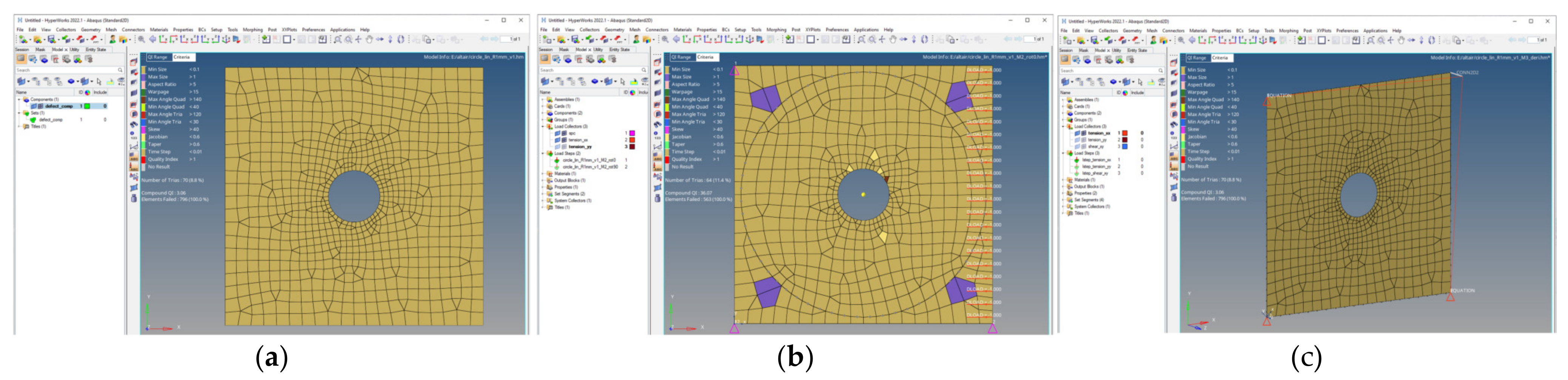
• The size of the surrounding bounding box of the input mesh should be about ten times the extent of the largest defect. The sub-case method splits the input model into a circular section, covering the corresponding defect geometries. The superposition method retains the initial mesh during evaluation.
• For planar models with mesh element count in the tens of thousands, the superposition method is more powerful, in terms of computation time. However, if the cell count is in the range of 100,000 or higher, the sub-case method is more applicable.
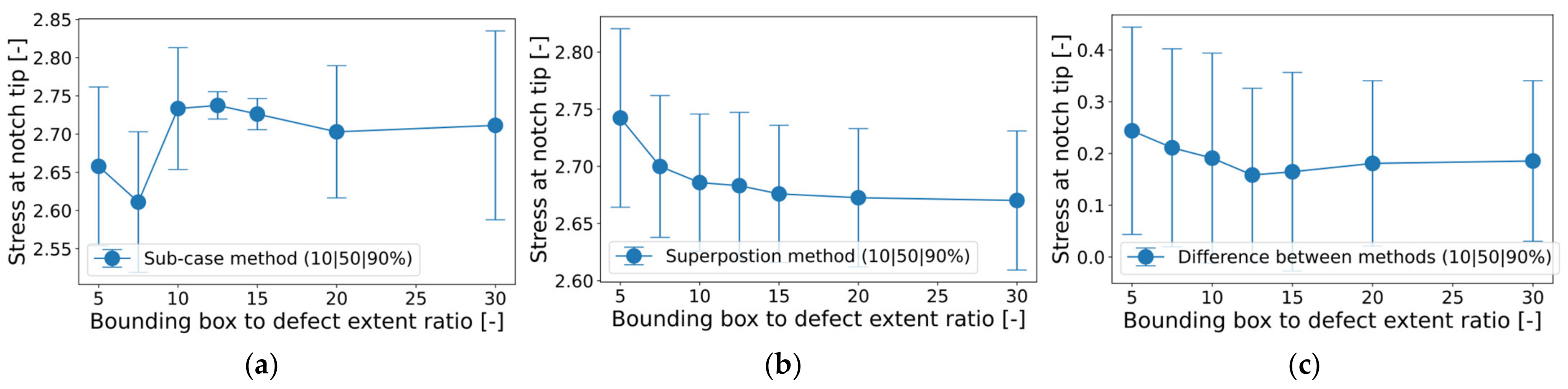
• If results with high accuracy are targeted, instead of minimizing the computation time, the sub-case method should be used for all fatigue approaches. The stress results obtained by the superposition method may differ by about 10–15%, depending on the evaluated notch geometry and mesh-seed. As the Point Method evaluates stress values at points away from the notch tip, the difference is less pronounced with this method. The same recommendations on method order hold true in the case of the elastic strain energy density approach, although the loss in accuracy with the superposition method is less pronounced compared to the sub-case method.
• The implemented methods are capable of evaluating not only a single pore, but also a network of pores concurrently. Thus, the imperfection distribution can be assessed efficiently.

Further work will focus on the extension of the introduced methods toward spatial fatigue assessment. For this purpose, the curvature assessment must be adapted, but the main working principle presented here holds. In addition, the corresponding load steps must be extended from the three basic cases for planar studies to six for spatial fatigue assessment. The tensor interpolation must be adopted, accordingly, but most of the numerical framework has already been designed for spatial fatigue evaluation.

Our currently ongoing work deals with experimental validation of the introduced numerically efficient methods on the basis of planar X-ray projections. Moreover, the advanced integration of the non-linear material behavior for total strain energy density evaluation is currently under study as well, which is expected to be integrated with the sub-case and superposition procedures shortly. This will extend the presented framework for strain energy density fatigue assessment towards the finite life region, paving the way to efficiently study the effect of variable amplitude service loads on single defects and imperfection networks.

References

1. Seeger, T.; Heuler, P. Generalized Application of Neuber’s Rule. J. Test. Eval. 1980, 8, 199–204. [Google Scholar] [CrossRef]
2. Radaj, D.; Sonsino, C.M.; Fricke, W. Fatigue Assessment of Welded Joints by Local Approaches, 2nd ed.; Woodhead: Cambridge, UK, 2006; ISBN 9780849384516. [Google Scholar]
3. Zhang, G. Method of effective stress for fatigue: Part I—A general theory. Int. J. Fatigue 2012, 37, 17–23. [Google Scholar] [CrossRef]
4. Zhang, G.; Sonsino, C.M.; Sundermeier, R. Method of effective stress for fatigue: Part II—Applications to V-notches and seam welds. Int. J. Fatigue 2012, 37, 24–40. [Google Scholar] [CrossRef]
5. Radaj, D.; Sonsino, C.M.; Fricke, W. Recent developments in local concepts of fatigue assessment of welded joints. Int. J. Fatigue 2009, 31, 2–11. [Google Scholar] [CrossRef]
6. Remes, H. Strain-based approach to fatigue crack initiation and propagation in welded steel joints with arbitrary notch shape. Int. J. Fatigue 2013, 52, 114–123. [Google Scholar] [CrossRef]
7. Vormwald, M. Effect of cyclic plastic strain on fatigue crack growth. Int. J. Fatigue 2016, 82, 80–88. [Google Scholar] [CrossRef]
8. Atzori, B.; Lazzarin, P.; Tovo, R. Stress distributions for V-shaped notches under tensile and bending loads. Fatigue Fract. Eng. Mater. Struct. 1997, 20, 1083–1092. [Google Scholar] [CrossRef]
9. Atzori, B. Cracks and notches: Analogies and differences of the relevant stress distributions and practical consequences in fatigue limit predictions. Int. J. Fatigue 2001, 23, 355–362. [Google Scholar] [CrossRef]
10. Atzori, B.; Lazzarin, P. Notch Sensitivity and Defect Sensitivity under Fatigue Loading: Two Sides of the Same Medal. Int. J. Fract. 2001, 107, 1–8. [Google Scholar] [CrossRef]
11. Atzori, B.; Lazzarin, P.; Meneghetti, G.; Buffière, J.Y.; Brune, M.; Morel, F.; Nadot, Y. A unifying approach to fatigue design in presence of defects and notches subject to uniaxial loading. MATEC Web Conf. 2014, 12, 9001. [Google Scholar] [CrossRef] [Green Version]
12. Schuscha, M.; Horvath, M.; Leitner, M.; Stoschka, M. Notch Stress Intensity Factor (NSIF)-Based Fatigue Design to Assess Cast Steel Porosity and Related Artificially Generated Imperfections. Metals 2019, 9, 1097. [Google Scholar] [CrossRef]
13. Schuscha, M.; Leitner, M.; Stoschka, M.; Pusterhofer, S.; Meneghetti, G. Numerical crack growth study on porosity afflicted cast steel specimens. Frat. Integr. Strutt. 2019, 13, 58–69. [Google Scholar] [CrossRef]
14. Taylor, D. The theory of critical distances. Eng. Fract. Mech. 2008, 75, 1696–1705. [Google Scholar] [CrossRef]
15. Susmel, L. The theory of critical distances: A review of its applications in fatigue. Eng. Fract. Mech. 2008, 75, 1706–1724. [Google Scholar] [CrossRef]
16. Meneghetti, G.; Lazzarin, P. The Peak Stress Method for Fatigue Strength Assessment of welded joints with weld toe or weld root failures. Weld. World 2011, 55, 22–29. [Google Scholar] [CrossRef]
17. Meneghetti, G.; Campagnolo, A.; Berto, F. Fatigue strength assessment of partial and full-penetration steel and aluminium butt-welded joints according to the peak stress method. Fatigue Fract. Eng. Mater. Struct. 2015, 38, 1419–1431. [Google Scholar] [CrossRef]
18. Lazzarin, P.; Lassen, T.; Livieri, P. A notch stress intensity approach applied to fatigue life predictions of welded joints with different local toe geometry. Fatigue Fract. Eng. Mater. Struct. 2003, 26, 49–58. [Google Scholar] [CrossRef]
19. Lazzarin, P.; Berto, F. Some Expressions for the Strain Energy in a Finite Volume Surrounding the Root of Blunt V-Notches. Int. J. Fract. 2005, 135, 161–185. [Google Scholar] [CrossRef]
20. Lazzarin, P.; Berto, F. Control volumes and strain energy density under small and large scale yielding due to tension and torsion loading. Fatigue Fract. Eng. Mater. Struct. 2008, 31, 95–107. [Google Scholar] [CrossRef]
21. Pittarello, L.; Campagnolo, A.; Berto, F. NSIFs estimation based on the averaged strain energy density under in-plane mixed mode loading. Procedia Struct. Integr. 2016, 2, 1829–1836. [Google Scholar] [CrossRef] [Green Version]
22. Atzori, B.; Ricotta, M.; Meneghetti, G. Strain energy-and stress-based approaches revisited in notch fatigue of ductile steels. MATEC Web Conf. 2018, 165, 14009. [Google Scholar] [CrossRef]
23. Beretta, S.; Murakami, Y. Statistical analysis of defects for fatigue strength prediction and quality control of materials. Fract. Eng. Mater. Struct. 1998, 21, 1049–1065. [Google Scholar] [CrossRef]
24. Murakami, Y. Material defects as the basis of fatigue design. Int. J. Fatigue 2012, 41, 2–10. [Google Scholar] [CrossRef]
25. Zerbst, U.; Madia, M.; Klinger, C.; Bettge, D.; Murakami, Y. Defects as a root cause of fatigue failure of metallic components. I: Basic aspects. Eng. Fail. Anal. 2019, 97, 777–792. [Google Scholar] [CrossRef]
26. Tiryakioğlu, M. Relationship between Defect Size and Fatigue Life Distributions in Al-7 Pct Si-Mg Alloy Castings. Metall. Mater. Trans. A 2009, 40, 1623–1630. [Google Scholar] [CrossRef]
27. Aigner, R.; Leitner, M.; Stoschka, M.; Hannesschläger, C.; Wabro, T.; Ehart, R. Modification of a Defect-Based Fatigue Assessment Model for Al-Si-Cu Cast Alloys. Materials 2018, 11, 2546. [Google Scholar] [CrossRef]
28. Aigner, R.; Pusterhofer, S.; Pomberger, S.; Leitner, M.; Stoschka, M. A probabilistic Kitagawa-Takahashi diagram for fatigue strength assessment of cast aluminium alloys. Mater. Sci. Eng. A 2019, 745, 326–334. [Google Scholar] [CrossRef]
29. Aigner, R.; Pomberger, S.; Leitner, M.; Stoschka, M. On the Statistical Size Effect of Cast Aluminium. Materials 2019, 12, 1578. [Google Scholar] [CrossRef]
30. Susmel, L.; Askes, H.; Bennett, T.; Taylor, D. Theory of Critical Distances versus Gradient Mechanics in modelling the transition from the short to long crack regime at the fatigue limit. Fatigue Fract. Eng. Mater. Struct. 2013, 36, 861–869. [Google Scholar] [CrossRef]
31. Susmel, L. A unifying approach to estimate the high-cycle fatigue strength of notched components subjected to both uniaxial and multiaxial cyclic loadings. Fatigue Fract. Eng. Mater. Struct. 2004, 27, 391–411. [Google Scholar] [CrossRef]
32. El Haddad, M.H.; Smith, K.N.; Topper, T.H. Fatigue Crack Propagation of Short Cracks. J. Eng. Mater. Technol. 1979, 101, 42–46. [Google Scholar] [CrossRef]
33. Kitagawa, H.; Takahashi, S. Applicability of fracture mechanics to very small cracks or the cracks in the early stage. In Proceedings of the Second International Conference on the Mechanical Behaviour of Materials, Boston, MA, USA, 6–20 August 1976; pp. 627–631. [Google Scholar]
34. Maierhofer, J.; Gänser, H.-P.; Pippan, R. Modified Kitagawa–Takahashi diagram accounting for finite notch depths. Int. J. Fatigue 2015, 70, 503–509. [Google Scholar] [CrossRef]
35. Susmel, L.; Taylor, D. A novel formulation of the theory of critical distances to estimate lifetime of notched components in the medium-cycle fatigue regime. Fatigue Fract. Eng. Mater. Struct. 2007, 30, 567–581. [Google Scholar] [CrossRef]
36. Ciavarella, M. A simple approximate expression for finite life fatigue behaviour in the presence of ‘crack-like’ or ‘blunt’ notches. Fatigue Fract. Eng. Mater. Struct. 2012, 35, 247–256. [Google Scholar] [CrossRef]
37. Susmel, L.; Taylor, D. A critical distance/plane method to estimate finite life of notched components under variable amplitude uniaxial/multiaxial fatigue loading. Int. J. Fatigue 2012, 38, 7–24. [Google Scholar] [CrossRef]
38. Horvath, M. Fatigue Life Assessment of Imperfective Cast Steel Components in the Medium-Cycle Regime by Stress- And Energy-Based Concepts. In Proceedings of the 6th International Conference on Structural Integrity and Durability, ICSID 2022, Dubrovnik, Croatia, 20–23 September 2022. [Google Scholar]
39. Williams, M.L. Stress Singularities Resulting from Various Boundary Conditions in Angular Corners of Plates in Extension. J. Appl. Mech. 1952, 19, 526–528. [Google Scholar] [CrossRef]
40. Meneghetti, G.; Lazzarin, P. Significance of the elastic peak stress evaluated by FE analyses at the point of singularity of sharp V-notched components. Fatigue Fract. Eng. Mater. Struct. 2007, 30, 95–106. [Google Scholar] [CrossRef]
41. Meneghetti, G.; Campagnolo, A.; Berto, F. Assessment of tensile fatigue limit of notches using sharp and coarse linear elastic finite element models. Theor. Appl. Fract. Mech. 2016, 84, 106–118. [Google Scholar] [CrossRef]
42. Meneghetti, G.; Campagnolo, A.; Avalle, M.; Castagnetti, D.; Colussi, M.; Corigliano, P.; de Agostinis, M.; Dragoni, E.; Fontanari, V.; Frendo, F.; et al. Rapid evaluation of notch stress intensity factors using the peak stress method: Comparison of commercial finite element codes for a range of mesh patterns. Fatigue Fract. Eng. Mater. Struct. 2017, 19, 526. [Google Scholar] [CrossRef]
43. Campagnolo, A.; Vecchiato, L.; Meneghetti, G. Multiaxial variable amplitude fatigue strength assessment of steel welded joints using the peak stress method. Int. J. Fatigue 2022, 163, 107089. [Google Scholar] [CrossRef]
44. Vecchiato, L.; Campagnolo, A.; Meneghetti, G. The Peak Stress Method for fatigue lifetime assessment of fillet-welded attachments in steel subjected to variable amplitude in-phase multiaxial local stresses. Int. J. Fatigue 2023, 169, 107482. [Google Scholar] [CrossRef]
45. Lazzarin, P.; Tovo, R. A unified approach to the evaluation of linear elastic stress fields in the neighborhood of cracks and notches. Int. J. Fract. 1996, 78, 3–19. [Google Scholar] [CrossRef]
46. Lazzarin, P.; Tovo, R. A notch intensity factor approach to the stress analysis of welds. Fract. Eng. Mater. Struct. 1998, 21, 1089–1103. [Google Scholar] [CrossRef]
47. Lazzarin, P.; Filippi, S. A generalized stress intensity factor to be applied to rounded V-shaped notches. Int. J. Solids Struct. 2006, 43, 2461–2478. [Google Scholar] [CrossRef]
48. Lazzarin, P.; Berto, F. From Neuber’s Elementary Volume to Kitagawa and Atzori’s Diagrams: An Interpretation Based on Local Energy. Int. J. Fract. 2005, 135, 33–38. [Google Scholar] [CrossRef]
49. Lazzarin, P.; Zambardi, R. A finite-volume-energy based approach to predict the static and fatigue behavior of components with sharp V-shaped notches. Int. J. Fract. 2001, 112, 275–298. [Google Scholar] [CrossRef]
50. Radaj, D. State-of-the-art review on extended stress intensity factor concepts. Fatigue Fract. Eng. Mater. Struct. 2014, 37, 1–28. [Google Scholar] [CrossRef]
51. Radaj, D. State-of-the-art review on the local strain energy density concept and its relation to the J-integral and peak stress method. Fatigue Fract. Eng. Mater. Struct. 2015, 38, 2–28. [Google Scholar] [CrossRef]
52. Meneghetti, G.; Campagnolo, A.; Berto, F.; Atzori, B. Averaged strain energy density evaluated rapidly from the singular peak stresses by FEM: Cracked components under mixed-mode (I+II) loading. Theor. Appl. Fract. Mech. 2015, 79, 113–124. [Google Scholar] [CrossRef]
53. Lazzarin, P.; Zambardi, R.; Livieri, P. Plastic notch stress intensity factors for large V-shaped notches under mixed load conditions. Int. J. Fract. 2001, 107, 361–377. [Google Scholar] [CrossRef]
54. Lazzarin, P.; Zappalorto, M. Plastic notch stress intensity factors for pointed V-notches under antiplane shear loading. Int. J. Fract. 2008, 152, 1–25. [Google Scholar] [CrossRef]
55. Lazzarin, P.; Zambardi, R. The Equivalent Strain Energy Density approach re-formulated and applied to sharp V-shaped notches under localized and generalized plasticity. Fatigue Fract. Eng. Mater. Struct. 2002, 25, 917–928. [Google Scholar] [CrossRef]
56. Zappalorto, M.; Lazzarin, P. Strain energy-based evaluations of plastic notch stress intensity factors at pointed V-notches under tension. Eng. Fract. Mech. 2011, 78, 2691–2706. [Google Scholar] [CrossRef]
57. Schuscha, M.; Leitner, M.; Stoschka, M.; Meneghetti, G. Local strain energy density approach to assess the fatigue strength of sharp and blunt V-notches in cast steel. Int. J. Fatigue 2020, 132, 105334. [Google Scholar] [CrossRef]
58. Branco, R.; Costa, J.D.; Borrego, L.P.; Berto, F.; Razavi, S.; Macek, W. Comparison of different one-parameter damage laws and local stress-strain approaches in multiaxial fatigue life assessment of notched components. Int. J. Fatigue 2021, 151, 106405. [Google Scholar] [CrossRef]
59. Li, X.-K.; Chen, S.; Zhu, S.-P.; Liao, D.; Gao, J.-W. Probabilistic fatigue life prediction of notched components using strain energy density approach. Eng. Fail. Anal. 2021, 124, 105375. [Google Scholar] [CrossRef]
60. Branco, R.; Prates, P.; Costa, J.D.; Cruces, A.; Lopez-Crespo, P.; Berto, F. On the applicability of the cumulative strain energy density for notch fatigue analysis under multiaxial loading. Theor. Appl. Fract. Mech. 2022, 120, 103405. [Google Scholar] [CrossRef]
61. Branco, R.; Martins, R.F.; Correia, J.; Marciniak, Z.; Macek, W.; Jesus, J. On the use of the cumulative strain energy density for fatigue life assessment in advanced high-strength steels. Int. J. Fatigue 2022, 164, 107121. [Google Scholar] [CrossRef]
62. Chang, D.; Yang, X.; Peng, H.; Hou, J.; Zuo, H. A critical elastic strain energy storage-based concept for characterizing crack propagation in elastic–plastic materials. Eng. Fract. Mech. 2022, 264, 108335. [Google Scholar] [CrossRef]
63. Li, J.; Wang, X.; Li, R.; Qiu, Y. Multiaxial fatigue life prediction for metals by means of an improved strain energy density-based critical plane criterion. Eur. J. Mech. A Solids 2021, 90, 104353. [Google Scholar] [CrossRef]
64. Ren, Z.; Qin, X.; Zhang, Q.; Sun, Y. Multiaxial fatigue life prediction model based on an improved strain energy density criterion. Int. J. Press. Vessels Pip. 2022, 199, 104724. [Google Scholar] [CrossRef]
65. Puri, G. Python Scripts for Abaqus: Learn by Example, 1st ed.; GB Books, Incr.: Hawthorne, CA, USA, 2011; ISBN 978-0-615520506. [Google Scholar]
66. Horvath, M.; Stoschka, M.; Fladischer, S. Fatigue strength study based on geometric shape of bulk defects in cast steel. Int. J. Fatigue 2022, 163, 107082. [Google Scholar] [CrossRef]
67. Gross, D.; Hauger, W.; Schröder, J.; Wall, W.A. Technische Mechanik; Springer: Berlin/Heidelberg, Germany, 2007; ISBN 978-3-540-70762-2. [Google Scholar]
68. Kaszynski, A.; Derrick, J.; Correia, D.; Addy, D. pyansys/pymapdl: V0.60.3. 2021. Available online: https://zenodo.org/record/5726008#.Y-SbTi9By3A (accessed on 21 November 2022).
69. Encyclopedia of Mathematics. Beta-Distribution. Available online: http://encyclopediaofmath.org/index.php?title=Beta-distribution&oldid=46045 (accessed on 21 November 2022).
70. Gupta, A.K.; Nadarajah, S. Handbook of Beta Distribution and its Applications; Marcel Dekker: New York, NY, USA, 2004; ISBN 978-0824753962. [Google Scholar]
71. Altair. HyperWorks: 2022.1. Available online: https://www.altair.com/hyperworks/ (accessed on 21 November 2022).
72. Nussbaumer, A.; Grigoriou, V. Round robin on local stress evaluation for fatigue by various FEM software: XIII-2650-19-R1. In Proceedings of the 69th International Institute for Welding (IIW) Annual Assembly and International Conference, Melbourne, Australia, 10–15 July 2016. 17p. [Google Scholar]
73. Altair. HyperMesh: 2022.1. Available online: https://www.altair.de/hypermesh/ (accessed on 21 November 2022).
74. Altair. HyperView: 2022.1. Available online: https://www.altair.de/hyperview/ (accessed on 21 November 2022).
75. Altair. Tcl/Tk Commands: 8.5.9. Available online: https://2021.help.altair.com/2021/hwdesktop/hwd/topics/reference/tcl/tcl_tk_syntax_r.htm (accessed on 21 November 2022).
76. Jones, K.; Welch, B. Practical Programming in Tcl and Tk, 4th ed.; Prentice Hall: Hoboken, NJ, USA, 2003; ISBN 0-13-038560-3. [Google Scholar]
77. Ousterhout, J.K. Tcl and the Tk Toolkit; Addison-Wesley: Boston, MA, USA, 2010; ISBN 978-0-321-33633-0. [Google Scholar]
78. VecTcL: 0.3. Available online: https://github.com/auriocus/VecTcl (accessed on 21 November 2022).
79. Altair. Compose: 2022.1. Available online: https://www.altair.com/compose (accessed on 21 November 2022).
80. OpenMatrix: 1.0.10. Available online: https://github.com/OpenMatrixLanguage/OpenMatrix (accessed on 21 November 2022).
81. Altair. Scripting Guide for the OpenMatrix Language: 2022.1. Available online: https://2021.help.altair.com/2021.2/compose/business/en_us/topics/language_guides/language_guide_intro_header_c.htm (accessed on 21 November 2022).
82. Altair. Use OML Function in HyperWorks Products: 2022.1. Available online: https://2021.help.altair.com/2021.2/compose/business/en_us/topics/compose/using_oml_functions_in_hyperworks_products_r.htm#using_oml_functions_in_hyperworks_products_r (accessed on 21 November 2022).
83. Altair. Templex Reference: 2022.1. Available online: https://2021.help.altair.com/2021/hwdesktop/hwd/topics/reference/templex/templex_overview_r.htm (accessed on 21 November 2022).
84. Altair. Object Hierarchy: 2022.1. Overview of Object Hierarchy for HyperView, HyperGraph, HyperWorks Desktop, MotionView, MediaView and TextView. 2022. Available online: https://2021.help.altair.com/2021/hwdesktop/hwd/topics/reference/tcl/object_hierarchy_r.htm (accessed on 21 November 2022).
85. Python 3.11.0 Documentation. Available online: https://docs.python.org/3/ (accessed on 21 November 2022).
86. Hellmann, D. The Python 3 Standard Library by Example; Addison-Wesley: Boston, MA, USA, 2017; ISBN 9780134291055. [Google Scholar]
87. Gorelick, M.; Ozsvald, I. High Performance Python: Practical Performant Programming for Humans, 2nd ed.; O’Reilly: Sebastopol, CA, USA, 2020; ISBN 1492055026. [Google Scholar]
88. Brownlee, J. Python Multiprocessing Jump-Start: Develop Parallel Programs, Side-Step the GIL, and Use All CPU Cores; Python Concurrency Jump-Start Series; Super Fast Python Pty. Ltd.: Vermont, VIC, Australia, 2022; ISBN 979-8842924988. [Google Scholar]
89. Altair. Compose-Usage Options: 2022.1. Business Edition. Available online: https://www.altair.com/compose-usage-options/ (accessed on 21 November 2022).
90. The HDF Group. HDF5: 1.10.9. Available online: https://portal.hdfgroup.org/display/HDF5/HDF5 (accessed on 21 November 2022).
91. Schroeder, W. The Visualization Toolkit: An Object-Oriented Approach to 3D Graphics, 4th ed.; Kitware: Clifton Park, NY, USA, 2006; ISBN 978-1-930934-19-1. [Google Scholar]
92. Sullivan, B.; Kaszynski, A.; Koyama, T.; Deak, A.; MatthewFlam; Favelier, G.; Jones, J.; Chiu, P.; Mologni, R.; Larson, E.; et al. pyvista/pyvista: Release Notes-v0.37.0; Zenodo: Geneva, Switzerland, 2023. [Google Scholar] [CrossRef]
93. Manfredo, P.D.C. Differential Geometry of Curves and Surfaces, Revised, 2nd ed.; Dover Publications Inc.: Mineola, NY, USA, 2016; ISBN 978-0-486-80699-0. [Google Scholar]
94. Halimi, O.; Raviv, D.; Aflalo, Y.; Kimmel, R. Computable invariants for curves and surfaces. In Processing, Analyzing and Learning of Images, Shapes, and Forms: Part 2; Elsevier: Amsterdam, The Netherlands, 2019; pp. 273–314. ISBN 9780444641403. [Google Scholar]
95. Batchelor, P. [vtkusers] Computing Curvature of a Surface. Available online: https://public.kitware.com/pipermail/vtkusers/2002-July/012198.html (accessed on 21 November 2022).
96. Cohen-Steiner, D.; Morvan, J.-M. Restricted delaunay triangulations and normal cycle. In Proceedings of the Nineteenth Conference on Computational Geometry—SCG ‘03. The Nineteenth Conference on Computational Geometry, San Diego, CA, USA, 8–10 June 2003; Fortune, S., Ed.; ACM Press: New York, NY, USA, 2003; p. 312, ISBN 1581136633. [Google Scholar]
97. VTK. vtkCurvatures Class Reference: 9.2.20221001. Available online: https://vtk.org/doc/nightly/html/classvtkCurvatures.html (accessed on 21 November 2022).
98. Carlson, K.; Ou, S.; Harin, R.A.; Beckermann, C. Analysis of ASTM X-ray shrinkage rating for steel castings. In Proceedings of the 54th SFSA Technical and Operating Conference, Chicago, IL, USA, 7–11 December 2022; Steel Founder’s Society of America: Crystal Lake, IL, USA, 2000; p. 35. [Google Scholar]
Figure 1. Dimensioned simulation results of a double V-notched plate (width W = 10 mm, opening angle 2α = 90°, notch depth a = 1 mm, unified tension loading): (a) Sharp notch (ρ = 0 mm); and (b) Blunt notch (ρ = 1 mm).
Applsci 13 02247 g001
Figure 2. Principle methods of solution to obtain local stress and elastic strain energy density results for irregularly shaped defects under uniaxial loading with varying load vectors: (a) Individual load case study; (b) Sub-case approach; and (c) Transformation and superposition of basic load steps.
Applsci 13 02247 g002
Figure 3. Numerical study of the applicability of peak stress method for sharp notches: (a) Parameter range; and (b) Comparison of the non-dimensional ratio K F E , I * and modified K F E , I , m o d * .
Applsci 13 02247 g003
Figure 4. Structured workflow for local fatigue assessment of planar imperfections.
Applsci 13 02247 g004
Figure 5. Setup of finite element models for both methods based on the same input mesh (circular hole-in-plate; referenced input mesh ‘circle_lin_R1mm_v1’): (a) Planar input mesh-pattern; (b) Re-meshed sub-case model with boundary conditions; and (c) Model of superposition method with boundary conditions and connectors.
Applsci 13 02247 g005
Figure 6. Displacement magnitude and principal stress results for different load angles φ (circular hole-in-plate; mesh ‘circle_lin_R1mm_v1’): (a) Sub-case approach; (b) Basic load cases; and (c) Superposition of derived basic load cases.
Applsci 13 02247 g006
Figure 7. Curvature workflow exemplified for different defect geometries: (a) Circular hole-in-plate (mesh ‘circle_lin_R1mm_v1’); (b) Elliptical hole-in-plate (mesh ‘ellipsis_lin_rot0deg_v1’); (c) Inclined elliptical hole-in-plate (mesh ‘ellipsis_lin_rot30deg_v1’); and (d) Elongated defect (mesh ‘defect_elongated_lin_v1’).
Applsci 13 02247 g007aApplsci 13 02247 g007b
Figure 8. Notch radius and notch opening angle for three defect geometries: (a) Circular hole-in-plate (mesh ‘circle_lin_R1mm_v1’); (b) Elliptical hole-in-plate (mesh ‘ellipsis_lin_rot0deg_v1’); and (c) Elongated defect (mesh ‘defect_elongated_lin_v1’).
Applsci 13 02247 g008
Figure 9. William’s eigenvalues and control volume distance for three defect geometries: (a) Circular hole-in-plate (mesh ‘circle_lin_R1mm_v1’); (b) Elliptical hole-in-plate (mesh ‘ellipsis_lin_rot0deg_v1’); and (c) Elongated defect (mesh ‘defect_elongated_lin_v1’).
Applsci 13 02247 g009
Figure 10. Computed vector paths for three defect geometries: (a) Circular hole-in-plate (mesh ‘circle_lin_R1mm_v1’); (b) Elliptical hole-in-plate (mesh ‘ellipsis_lin_rot0deg_v1’); and (c) Elongated defect (mesh ‘defect_elongated_lin_v1’).
Applsci 13 02247 g010
Figure 11. Fraction of cells at starting point for three defect geometries: (a) Circular hole-in-plate (mesh ‘circle_lin_R1mm_v1’); (b) Elliptical hole-in-plate (mesh ‘ellipsis_lin_rot0deg_v1’); and (c) Elongated defect (mesh ‘defect_elongated_lin_v1’).
Applsci 13 02247 g011
Figure 12. Notch tip stress evaluation of circular hole-in-plate (mesh ‘circle_lin_R1mm_v1’) by sub-case and superposition methods for incremental load step of Δ φ = 5 ° : (a) Level plots; and (b) Course along defect contour.
Applsci 13 02247 g012
Figure 13. Notch tip stress evaluation of elliptical hole-in-plate (mesh ‘ellipsis_lin_rot0deg_v1’) by sub-case and superposition methods for incremental load step of Δ φ = 5 ° : (a) Level plots; and (b) Course along defect contour.
Applsci 13 02247 g013
Figure 14. Notch tip stress evaluation of elliptical hole-in-plate (mesh ‘defect_elongated_lin_v1’) by sub-case and superposition methods for incremental load step of Δ φ = 5 ° : (a) Level plots; and (b) Course along defect contour.
Applsci 13 02247 g014
Figure 15. Assessment of maximum notch tip stress of circular hole-in-plate with increased bounding box (mesh list ‘circle_lin_R1mm_v1,v2…v7’) for incremental load step of Δ φ = 10 ° : (a) Sub-case method; (b) Superposition method; and (c) Difference between these methods.
Applsci 13 02247 g015
Figure 16. N-SIF peak stress course for three defect geometries, assuming a sharp notch and incremental load step of Δ φ = 10 ° : (a) Circular hole-in-plate (mesh ‘circle_lin_R1mm_v1’); (b) Elliptical hole-in-plate (mesh ‘ellipsis_lin_rot0deg_v1’); and (c) Elongated defect (mesh ‘defect_elongated_lin_v1’).
Applsci 13 02247 g016
Figure 17. N-SIF peak stress course for three defect geometries assuming a blunt notch and incremental load step of Δ φ = 10 ° : (a) Circular hole-in-plate (mesh ‘circle_lin_R1mm_v1’); (b) Elliptical hole-in-plate (mesh ‘ellipsis_lin_rot0deg_v1’); and (c) Elongated defect (mesh ‘defect_elongated_lin_v1’).
Applsci 13 02247 g017
Figure 18. PSM peak stress course for three defect geometries and incremental load step of Δ φ = 10 ° : (a) Circular hole-in-plate (mesh ‘circle_lin_R1mm_v1’); (b) Elliptical hole-in-plate (mesh ‘ellipsis_lin_rot0deg_v1’); and (c) Elongated defect (mesh ‘defect_elongated_lin_v1’).
Applsci 13 02247 g018
Figure 19. Evaluation of maximum TCD Point Method stresses of a circular hole-in-plate model with increasing arc-lengths and incremental load step of Δ φ = 3 ° : (a) Sub-case method; and (b) Superposition method.
Applsci 13 02247 g019
Figure 20. TCD Point Method stress course for three defect geometries at evaluation arc-length L m = a 0 / 2 = 0.113   mm and incremental load step of Δ φ = 10 ° : (a) Circular hole-in-plate (mesh ‘circle_lin_R1mm_v1’); (b) Elliptical hole-in-plate (mesh ‘ellipsis_lin_rot0deg_v1’); and (c) Elongated defect (mesh ‘defect_elongated_lin_v1’).
Applsci 13 02247 g020
Figure 21. TCD Point Method stress course for three defect geometries at evaluation arc-length L m = 1   mm and incremental load step of Δ φ = 10 ° : (a) Circular hole-in-plate (mesh ‘circle_lin_R1mm_v1’); (b) Elliptical hole-in-plate (mesh ‘ellipsis_lin_rot0deg_v1’); and (c) Elongated defect (mesh ‘defect_elongated_lin_v1’).
Applsci 13 02247 g021
Figure 22. Comparison of blunt notched V-plate (mesh ‘K1V_H10_A1_PHI90_RHO1_E_TE’) and circular hole-in-plate (mesh ‘circle_fine_quad_R1mm_v1’): (a) Absolute max principal stress; and (b) Displacement in the x-axis.
Applsci 13 02247 g022
Figure 23. ESED evaluation of fine-meshed circular hole-in-plate (mesh ‘circle_fine_quad_R1mm_v1’) by sub-case method and incremental load step of Δ φ = 3 ° : (a) Level plot; and (b) Plots along defect contour.
Applsci 13 02247 g023
Figure 24. ESED evaluation of coarse-meshed circular hole-in-plate (mesh ‘circle_lin_R1mm_v1’) by sub-case method and incremental load step of Δ φ = 15 ° : (a) Level plot; and (b) Plots along defect contour.
Applsci 13 02247 g024
Figure 25. ESED evaluation of coarse-meshed circular hole-in-plate (mesh ‘circle_lin_R1mm_v1’) by scalar superposition: (a) Contour plots for load angle of φ = 0 ,   45 ,   90 ,   135 ° ; and (b) ESED plots along defect contour.
Applsci 13 02247 g025
Figure 26. ESED evaluation of coarse-meshed circular hole-in-plate (mesh ‘circle_lin_R1mm_v1’) by tensor superposition: (a) Stress contour plots; (b) Strain contour plots; and (c) Elastic strain energy density contour plots for load angle of φ = 0 ,   45 ,   90 ,   135 ° .
Applsci 13 02247 g026
Figure 27. ESED course for three defect geometries, evaluated as sharp notch and with incremental load step of Δ φ = 10 ° : (a) Circular hole-in-plate (mesh ‘circle_lin_R1mm_v1’); (b) Elliptical hole-in-plate (mesh ‘ellipsis_lin_rot0deg_v1’); and (c) Elongated defect (mesh ‘defect_elongated_lin_v1’).
Applsci 13 02247 g027
Figure 28. ESED course for three defect geometries evaluated as blunt notch and with incremental load step of Δ φ = 10 ° : (a) Circular hole-in-plate (mesh ‘circle_lin_R1mm_v1’); (b) Elliptical hole-in-plate (mesh ‘ellipsis_lin_rot0deg_v1’); and (c) Elongated defect (mesh ‘defect_elongated_lin_v1’).
Applsci 13 02247 g028
Figure 29. Example of TCD evaluation of pore network following ASTM Standard E446 classA1 applying the sub-case method (mesh ‘ASTM_A1_quad_v1’): (a) Contour plots for load angle φ = 100 ° ; and (b) Course of evaluated Point Method stress values and load angle per defect.
Applsci 13 02247 g029