A Glaucoma Detection System Based on Generative Adversarial Network and Incremental Learning

Abstract

Among various eye diseases, glaucoma is one of the leading causes of blindness. Glaucoma is also one of the most common eye diseases in Taiwan. Glaucoma screenings can use optical coherence tomography (OCT) to locate areas in which the retinal nerve fiber layer is thinning. However, because OCT equipment is costly, only large hospitals with well-equipped facilities will have OCT, and regular eye clinics cannot afford such expensive equipment. This has caused many glaucoma patients to worsen because they cannot get an early diagnosis in regular eye clinics in time. This paper proposes a method of using a generative adversarial network (GAN) to generate corresponding OCT images from fundus images to assist family doctors in judging whether further examination is needed based on the generated OCT images to achieve early detection and treatment of glaucoma. In addition, in order to improve the classification accuracy of the system deployed in different hospitals or clinics, this paper also proposes to use the incremental training method to fine-tune the model. The model can be quickly applied by adding a small number of images from a specific clinic or hospital. Experimental results show that the cosine similarity between the generated OCT image and the real OCT image is 97.8%. Combined with the proposed transfer learning method, the classification accuracy of the classification model reaches 83.17%. As well as the use of the incremental method, the accuracy of identifying glaucoma is approximately 78.94%, which is 8.77% higher than the 70.17% accuracy of the initial model. Experimental results show the effectiveness and feasibility of our proposed method.

1. Introduction

Glaucoma, a type of optic nerve damage that can cause vision impairment and lead to blindness, is the second most common cause of blindness worldwide. According to the World Health Organization (WHO), more than 76 million people suffered from glaucoma in 2020, which is expected to increase to 111.8 million by 2040 [1]. Because glaucoma has no noticeable symptoms in the early stage, it is nicknamed the silent thief of sight [2], and 90% of glaucoma is not detected early. If glaucoma patients are not diagnosed and treated in time, they may be permanently blind as the optic nerve is damaged. It is crucial to develop glaucoma detection systems for early diagnosis.

Glaucoma is mainly related to high intraocular pressure, which can cause damage to the optic nerve. As the optic nerve degenerates, glaucoma patients’ vision gradually narrows, eventually leading to blindness. Therefore, it is essential to monitor intraocular pressure at any time and use instruments to diagnose glaucoma and evaluate changes in the optic nerve objectively.

To accurately diagnose glaucoma, ophthalmologists will conduct a series of examinations for patients in clinical diagnosis, including:

(1)

Intraocular pressure test: The normal intraocular pressure is 10–21 mmHg. When the intraocular pressure is higher than 22 mmHg, the risk of glaucoma is higher.

(2)

Visual field test: Visual field refers to the range that the eyes can see. Standard Automated Perimetry (SAP) can describe the visual field of the patient’s eyes. When a defect in the central visual field or the peripheral visual field narrows, it may be a symptom of glaucoma.

(3)

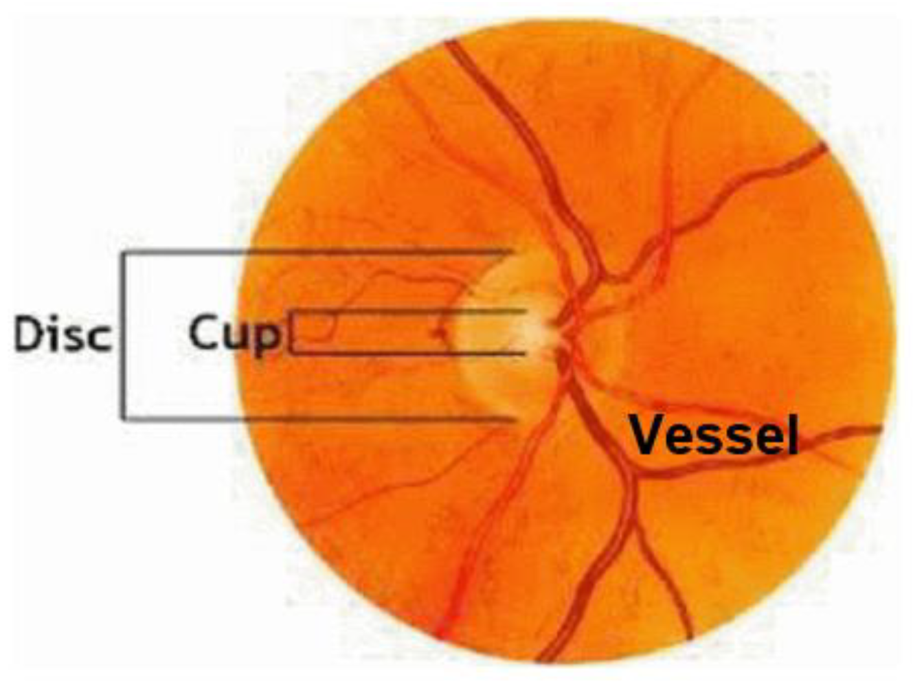
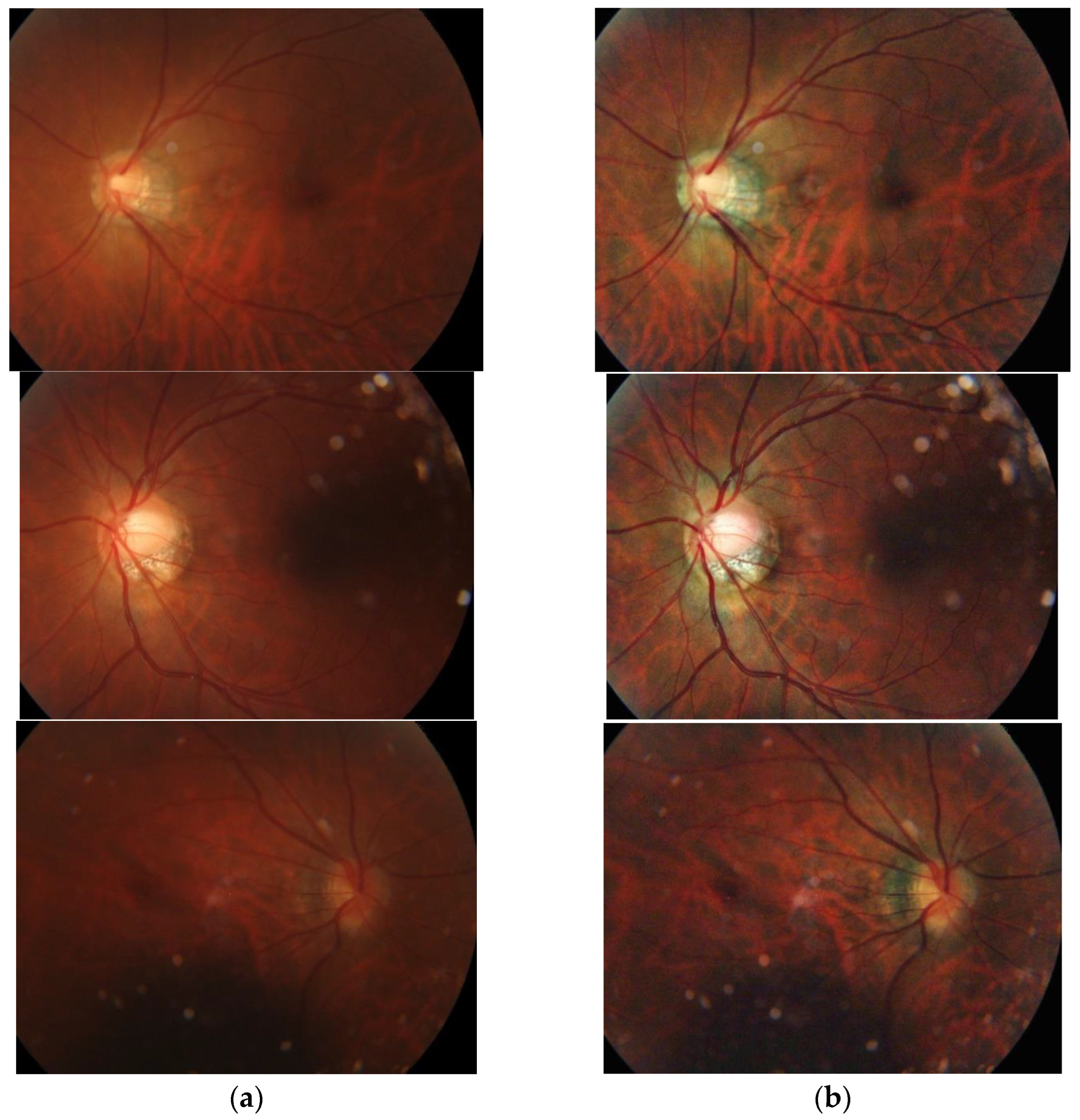
Fundus photography: In both normal people and people with abnormal optic nerves, the vast majority have optic disc depressions, but the depression of optic discs in glaucoma patients will increase or show different changes with the disease. Experienced ophthalmologists use fundus photography to screen patients for possible glaucoma. Figure 1 shows fundus OCT images of (a) healthy and (b) unhealthy retinas [3]. The fundus image and the important parts of the eye are marked in Figure 2.

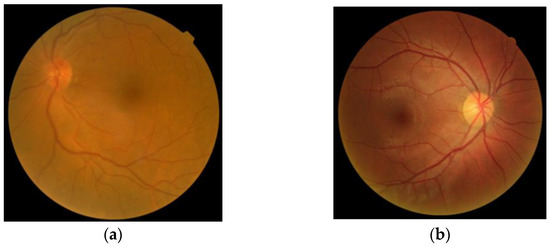Figure 1. Fundus images: (a) Healthy, (b) Glaucomatous.

Figure 2. Sample fundus image with the main anatomic parts.

(4)

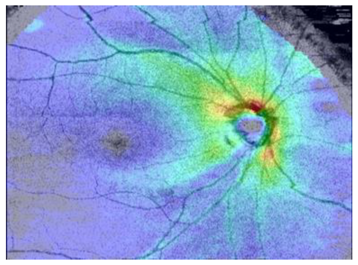
Optical coherence tomography (OCT) examination: using optical principles to conduct cross-sectional analysis of the cornea, iris, lens, retina, optic disc, optic nerve, etc., in a non-invasive manner [3,4], as shown in Figure 3. OCT can objectively measure the thickness of the optic nerve fiber layer to assist in the early diagnosis of glaucoma. Ophthalmologists can also analyze the previous OCT images of patients to check for changes in the optic nerve to monitor and control the glaucoma condition.

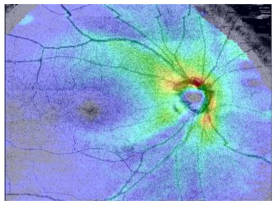Figure 3. An OCT image.

The quality and resolution of OCT images have given it the nickname optical biopsy in some literature [5]. However, in eye disease diagnosis, fundus photography and optical tomography (OCT) are usually not performed on the patient simultaneously. Generally, the ophthalmologist will take further OCT scanning actions when they detect any abnormalities from the prior fundus photography.

The symptoms of glaucoma are not apparent in the early stage, and it is usually not easy to discover. Because OCT equipment is expensive, it is not easy for small ophthalmology clinics to afford it. Usually, only large hospitals can do in-depth OCT examinations for glaucoma.

The use of computer-aided diagnosis in the screening and diagnosis of glaucoma from fundus or OCT images has become a trend with the advancement of information technology. Developing a tool for computer-aided detection of glaucoma with a high sensitivity and low false positive rate can help ophthalmologists to provide a positive clinical diagnosis.

Therefore, this study hopes that the fundus photography and imaging equipment can generate OCT images while taking pictures to facilitate doctors’ diagnosis and preventive treatment of glaucoma. This paper proposes a glaucoma identification method that combines generative adversarial networks and incremental learning. Utilizing techniques from generative adversarial networks, the proposed system can generate OCT images using only fundus images. The incremental training architecture based on transfer learning allows us to quickly train classification models in different fields. The integrated glaucoma recognition system will enable doctors to use the generated images to determine whether a patient has glaucoma. This system can assist doctors in making correct judgments and also simplifies the screening process.

Every hospital has different medical equipment from different brands and settings, so the generated images will have different qualities. When deploying the classification system in various hospitals, images with different quality will reduce the accuracy of the classification model. We propose a method that uses incremental training to fine-tune the model by adding a small number of images from a specific field to quickly and accurately apply the model.

In this paper, we integrated the GAN model and incremental learning technology for glaucoma detection. We conclude the main contributions of this paper are as follows:

• The proposed method, in addition to the system’s high accuracy, can also be quickly deployed in different fields.
• The developed glaucoma detection software has been clinically implemented in the Department of Glaucoma, Chang Gung Memorial Hospital, Taiwan, to assist doctors in interpreting glaucoma in fundus images.
• Glaucoma can be detected by fundus images and the proposed glaucoma detection software without needing expensive OCT equipment.

The rest of this paper is organized as follows. Section 2 briefly describes the related research. We describe the proposed method in detail in Section 3 and we present the experimental results and further explain and discuss the results in Section 4. Finally, we conclude this paper in Section 5.

2. Related Work

With the rapid development of deep learning technology and high-speed computing hardware, many researchers have successively invested in computer-aided diagnosis (CAD) systems for various diseases. For example, Heidari et al. [6,7] proposed a system for detecting COVID-19, Suryani et al. [8] proposed a lung cancer diagnosis system, Shen et al. [9] proposed a breast cancer detection system, etc. CAD systems are crucial in modern clinics to guide the accurate detection and treatment of different diseases. It plays an outstanding role in disease detection, clinical diagnosis, and treatment planning.

Glaucoma is an incurable eye disease that causes retinal degeneration. Although glaucoma cannot be cured completely, its progression can be controlled if diagnosed early. Unfortunately, early diagnosis is rare because there are no apparent symptoms in the early stage. Several researchers have attempted to investigate various methods and algorithms for glaucoma detection using fundus images.

Abdullah et al. [10] described several computer-based methods for glaucoma detection. They also introduce various datasets, such as SINDI, SCES, and SIMES, and methodologies for detecting glaucoma, such as detection of glaucoma through optic nerve head, thresholding-based techniques, and level-set-based techniques.

Thakur et al. [11] analyzed different researchers’ optic disc and optic cup segmentation methods and their classification in glaucoma diagnosis.

Maheshwari et al. [12] proposed an automatic glaucoma diagnosis method. They use empirical wavelet transform (EWT) on digital images for image decomposition and extract the desired features with correlation entropy, then use the least squares SVM (LS_SVM) to construct the classifier.

The glaucoma detection system proposed by Acharya et al. [13] converts color images to grayscale images with adaptive histogram equalization, and then convolutes these images with Leung-Malik (LM), Schmid (S) and maximum response (MR4 and MR8) filters. These convoluted textures are used to extract Local Configuration Pattern (LCP) features, followed by k-Nearest Neighbors (kNN) for classification.

A method for optic disc (OD) segmentation based on multi-level thresholding was proposed by Kankanala et al. [14] Retinal vessels are enhanced by convolving the image with a linear filter, and ROIs are achieved by applying a local entropy threshold. To segment OD regions, they implemented multilevel thresholding followed by morphological operations. However, in this technique, the segmentation of OC, which is also essential for glaucoma disease screening, is not considered.

Convolutional neural networks (CNNs) are able to obtain information in hierarchical structures from images and thus can be applied to distinguish glaucomatous images from non-glaucoma images. Mamta et al. [15] proposed an enhanced U-Net model called G-Net to implement their glaucoma detection system, which is based on the deep learning structure developed by CNNs.

A generative adversarial network (GAN) [16] consists of a generator and a discriminator whose purpose is to generate new data similar to some input data. The generator tries to generate data that can fool the discriminator, and the discriminator tries to correctly identify the generated data as fake. Bisneto et al. [17] trained a conditional generative adversarial network (cGAN) to segment discs from retinal images to detect glaucoma. They used taxonomic diversity and distinction indices to distinguish and classify abnormalities in retinal images. Saeed et al. [18] reviewed the literature on the use of GAN technology to diagnose eye diseases in recent years. They described the advantages and disadvantages of this technology as well as future trends.

Since 1995, research on transfer learning has attracted a lot of attention and has gone by different names, such as learning to learn, lifelong, knowledge transfer, inductive transfer, multitask learning, knowledge consolidation, context-sensitive learning, knowledge-based inductive bias, meta learning, and incremental/cumulative learning [19].

Incremental learning is a machine learning technique in which a model is trained to learn new tasks over time without forgetting previously learned tasks. The main idea is to train a model incrementally by adding new tasks one at a time rather than retraining the model from scratch for each task. [20].

The primary method of incremental learning is to use a pre-trained model as the starting point for a new model, and then fine-tune the model on the new task using a smaller dataset. This process involves freezing the weights of some or all of the layers of the pre-trained model, and then training the remaining layers on the new task. The pre-trained model can be fine-tuned by adjusting the parameters of the model. This can be done by unfreezing some layers and training them further or adding new layers to the model. The fine-tuning process can be performed on the entire dataset, a subset, or even on a new dataset.

In this paper, we propose a method to detect glaucoma from fundus images only, without expensive OCT equipment, and with high accuracy. In addition, when we deploy the glaucoma detection system in different fields, we use the incremental learning framework based on transfer learning to improve accuracy and shorten the time for system deployment and fine-tuning. The proposed system can be an invaluable tool for physicians, helping them improve the quality of diagnoses they provide to their patients.

3. Methodology

This section will introduce our proposed glaucoma detection system, including the system architecture and operation process. We will present the details of image preprocessing, fundus-to-OCT generator, and glaucoma classifier in the following subsections.

3.1. The Proposed System Architecture for Glaucoma Detection

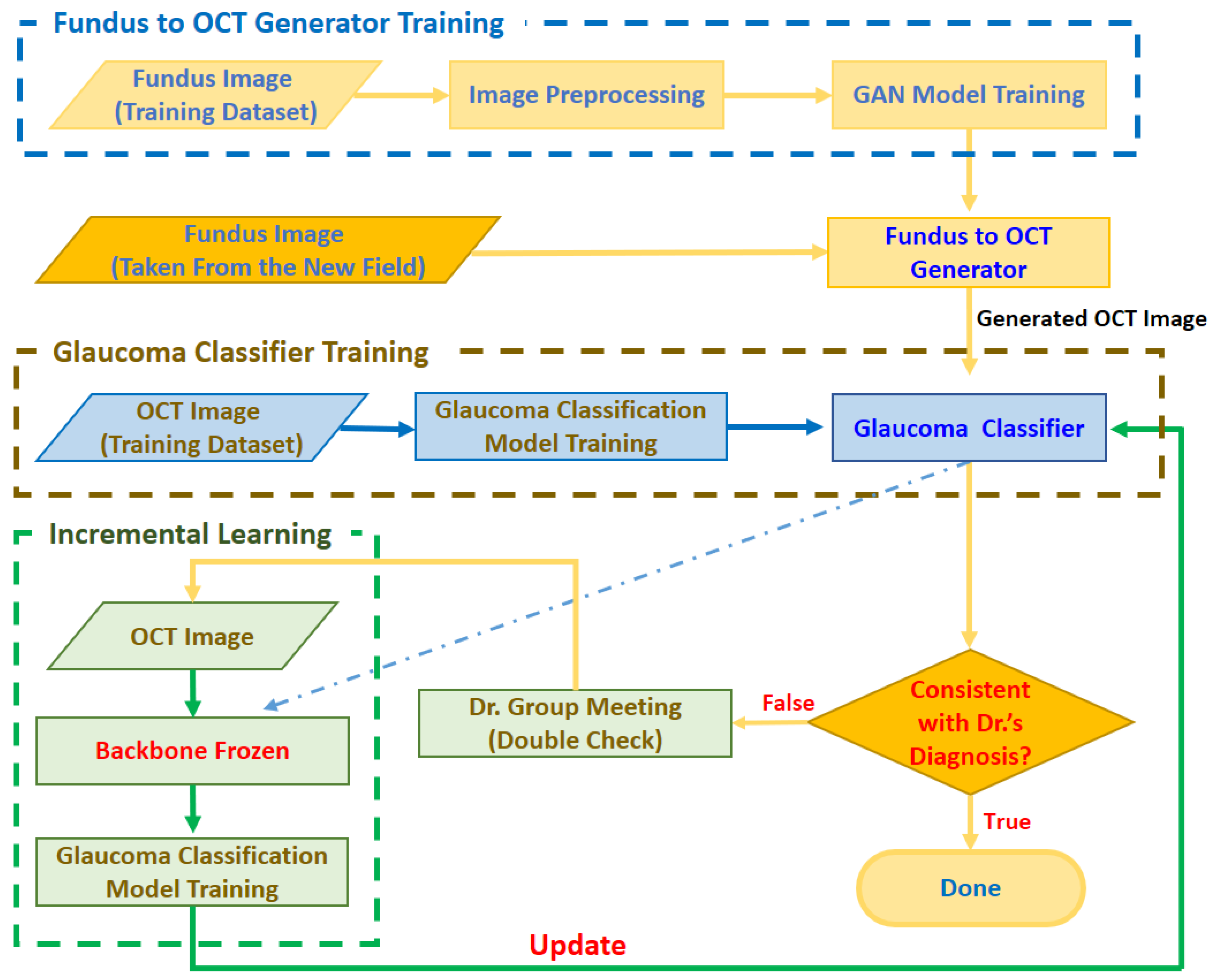
As shown in Figure 4, the glaucoma detection system consists of the following three stages:

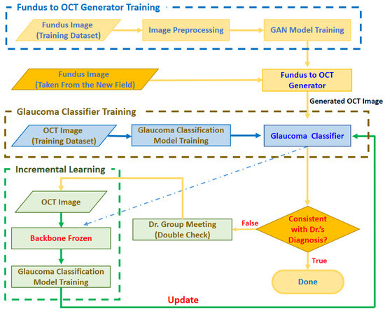
Figure 4. Architecture of the proposed glaucoma detection system.

• Stage 1. Fundus to OCT Generator Training

In order to judge whether there are glaucoma symptoms through the fundus image, the system will first train the fundus to OCT generator with the fundus image provided by the ophthalmologist and the corresponding OCT image. The trained generator can output a realistic OCT image corresponding to the input image based on the input fundus image.

• Stage 2. Glaucoma Classifier Training

In order to correctly classify glaucoma from OCT images, at this stage, we train the glaucoma classifier with OCT images marked by ophthalmologists. The trained glaucoma classifier can judge whether it is glaucoma according to the input OCT image.

• Stage 3. Incremental Learning

When deploying the trained Fundus to OCT Generator and Glaucoma Classifier to a new field, the image quality may be inconsistent due to different brands and settings of the fundus photography equipment, resulting in low accuracy of the model. Therefore, we use fundus images from new fields to fine-tune the glaucoma classifier based on the spirit of incremental learning. The general process is as follows: when the fundus image obtained from the new field is input to the generator, the generator will output the corresponding OCT image and then feed the OCT image to the glaucoma classifier. When the classifier’s output is inconsistent with the doctor’s diagnosis, a small expert meeting will be held. Through discussions with other doctors, the fundus image and the generated OCT image will be re-judged, labeled, trained, and the glaucoma classifier will be adjusted.

3.2. Image Preprocessing

Since the Fundus images captured by the fundus camera contain many black borders, and because of the different settings of the shooting equipment, the brightness and darkness are inconsistent. As shown in Figure 5, in order to improve the generation quality of the image generation model, each fundus image will be pre-processed in the following four steps:

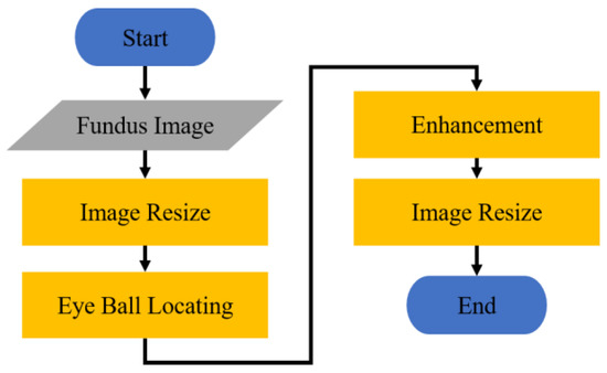
Figure 5. Flowchart of image preprocessing.

(1)

Scale down the fundus image to 20% of the original image.

(2)

Find out the location of the eyeball from the fundus image, and crop the image.

(3)

Enhance the cropped fundus image.

(4)

Resize the enhanced image to 256 × 256.

3.2.1. Image Resizing

The size of the fundus image obtained by the fundus camera is 2576 × 1934. This huge image will increase the amount of calculation when doing the Hough transform [21]. Therefore, before eyeball locating, we remove the black border of the image and then scale down the image with the black border removed to 20% of the original image. The width of the fundus image processed at this stage is 512. In order to speed up the model training, the system further resizes the enhanced image to 256 × 256 for subsequent model training.

3.2.2. Eyeball Locating

Hough Transform [21] is one of the primary methods for recognizing geometric shapes in image processing, and it is mainly used to extract geometric shapes with similar features in images. Because the area of the fundus in the captured fundus image is a circle, in this stage, we use the Hough transform to easily locate the part of the fundus.

As shown in Figure 6, we make the circle found by the Hough transform into an image mask with the same size as the fundus image. Then, the fundus image is cropped according to the position of the eyeball in the OCT image with this mask to filter out unimportant parts of the image, as shown in Figure 7. Figure 8 shows the fundus image overlaid with an image mask and the original OCT image.

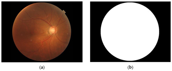
Figure 6. (a) Fundus image. (b) Image mask.

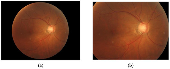
Figure 7. (a) Fundus image overlaid with an image mask. (b) Cropped fundus image.

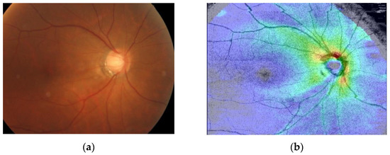
Figure 8. (a) Fundus image overlaid with an image mask. (b) Original image of OCT image.

3.2.3. Image Enhancement

In order to make the training image clearer, we use the Contrast Limited Adaptive Histogram Equalization (CLAHE) method [22], which can enhance the contrast of the fundus image and make the details in the fundus image clearer. Figure 9 shows three enhanced fundus images. The image on the left is the original image, while CLAHE enhances the image on the right.

Figure 9. Comparison of before and after image enhancement: (a) Fundus image without enhancement. (b) Fundus image with enhancement.

3.3. Image Generation

Generative adversarial network (GAN) [16] is one of the recent most highly discussed deep learning models. GAN is a deep neural network architecture composed of two networks, a generator (G) and a discriminator (D). Its core logic is that the generator and the discriminator will enhance each other’s capabilities through an adversarial process. In this paper, we propose a deep generative adversarial model for converting fundus images to OCT images based on the spirit of GAN.

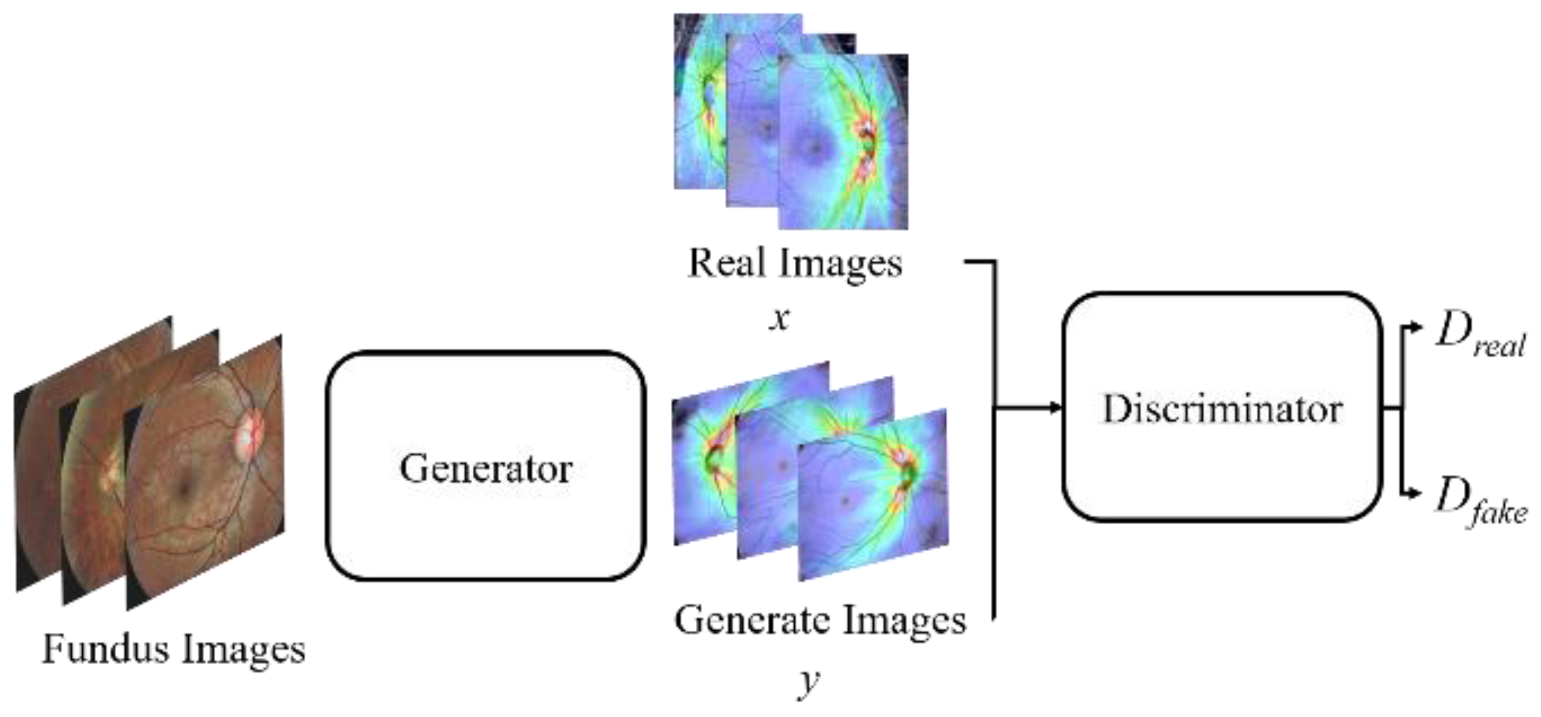
Figure 10 shows a schematic diagram of our proposed GAN. The training process of the proposed GAN model is to train the discriminator first, and then train the generator. In order for the discriminator to learn a criterion that can distinguish between real and fake (generated) images, during discriminator training, a lot of real OCT images x are provided and fed into the discriminator. Furthermore, the fundus image is fed into the generator to generate the corresponding OCT image y. Then, we composite the generated OCT image y with real OCT images x as the input of the discriminator for discrimination. The discriminator will judge whether the composite image is real or fake (generated) according to the criteria obtained from the previous training. If the composite image is judged to be real, the image will be assigned a higher score (nearly 1), conversely, if it is judged to be a fake (generated) image, the image will be assigned a lower score (nearly 0). Then, the weights are adjusted and the process is repeated until the discriminator cannot distinguish between real and generated images. This means that the generator has been able to create a diverse set of OCT images that are highly similar to real images.

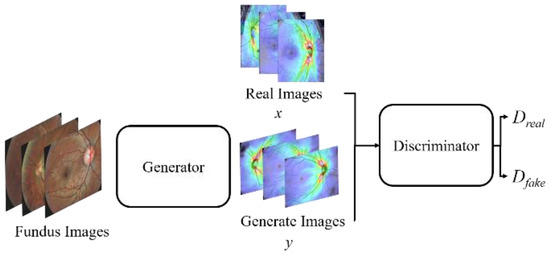
Figure 10. A schematic diagram of the proposed GAN model.

3.3.1. The Architecture of the OCT Generator

Figure 11 shows the architecture of the image generation model. In order to avoid the problem of loss of details in image generation, we refer to the concept of U-Net feature channels, and concat the features extracted by the second and third convolutional layers of the encoder to the corresponding convolutional layers of the decoder.

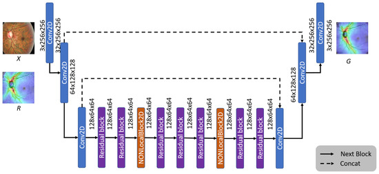
Figure 11. The architecture of the OCT generator model.

Since the convolutional neural network (CNN) [23] calculates the local area’s features, most of the feature loss problems can be solved through feature splicing. Furthermore, to retain more details in the generation stage, we add Non-Local Blocks [24] to the generative model to strengthen the information relationship between each pixel, allowing the generator to generate more realistic images.

In this paper, the real and generated OCT images are denoted by x and y, respectively. We divide each image into 11 × 11 blocks and use the average value of image brightness (l), contrast (c), and structure (s) as the evaluation criteria, where M represents the number of image blocks.

The multiscale structural similarity (MS-SSIM) [25] is adopted as the loss function for the generator model to evaluate the image quality objectively. The MS-SSIM is defined by Equation (1):

$$L\left(x,y\right)={l\left(x_M,y_M\right)}^M\cdot {\prod }_{j=1}^M{c\left(x_j,y_j\right)}^j{s\left(x_j,y_j\right)}^j,$$

(1)

Using Equation (1), the quality of the generated image can be determined, with a higher score representing a higher similarity.

The brightness index equation is defined as:

$$l\left(x,y\right)=\frac{2{\mu }_x{\mu }_y+C_1}{{\mu }_x^2+{\mu }_y^2+C_1},$$

(2)

where μ_x and μ_y are the average pixel values of the real and generated images x and y, respectively, and C₁ is a constant added to prevent the denominator from approaching zero.

The image contrast index equation is defined as:

$$c\left(x,y\right)=\frac{2{\sigma }_x{\sigma }_y+C_2}{{\sigma }_a^2+{\sigma }_y^2+C_2},$$

(3)

where σ_x and σ_y are the pixel standard deviations of the real and generated images x and y, and C₂ is a constant added to prevent the denominator from approaching zero.

The structural index equation is defined as:

$$s\left(x,y\right)=\frac{{\sigma }_{xy}+C_3}{{\sigma }_x{\sigma }_y+C_3},$$

(4)

where σ_xy is the covariance of the real and generated images x and y, and C₃ is a constant added to prevent the denominator from approaching zero.

The Loss function of the generator is defined as:

$$GeneratorLoss=1-L(x,y),$$

(5)

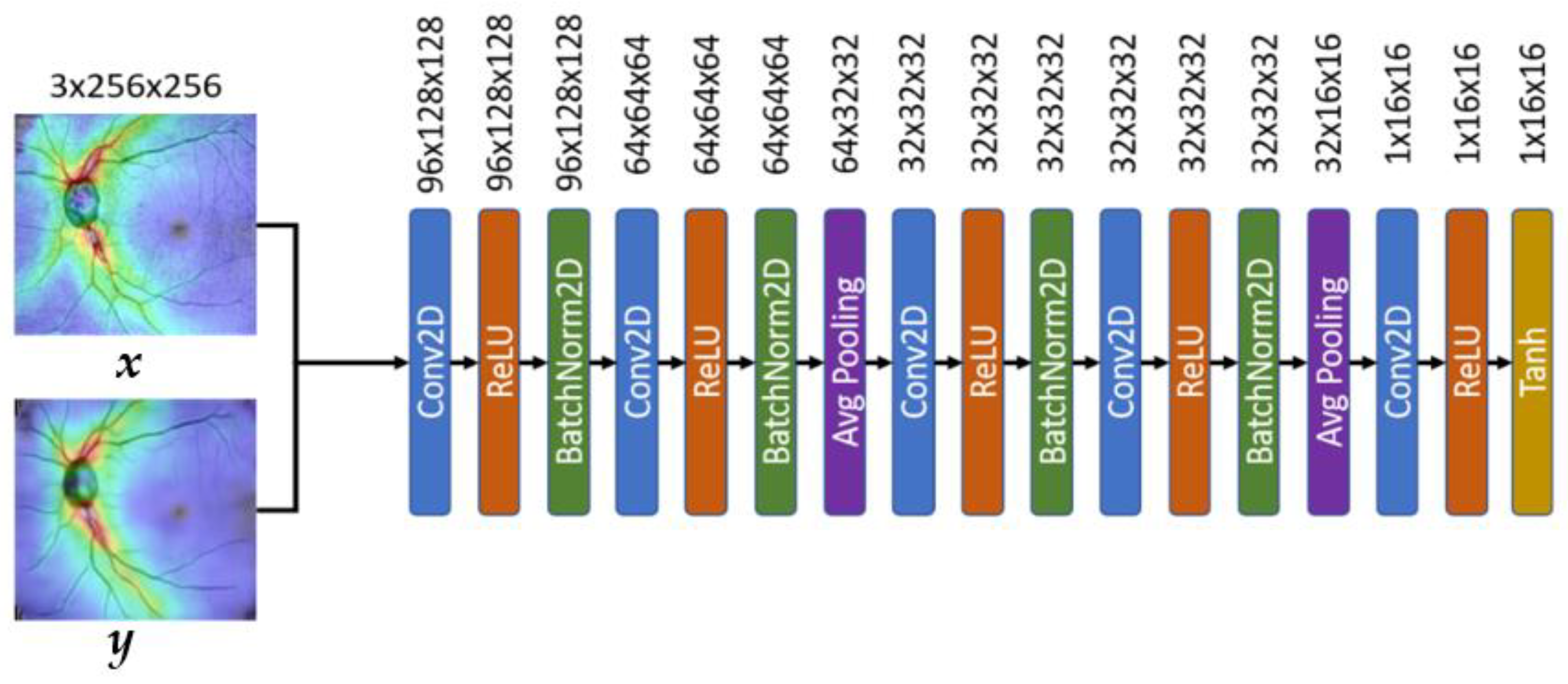
3.3.2. The Architecture of the OCT Discriminator

As shown in Figure 12, the proposed system uses the Markov Discriminator [26] as the discriminator. The difference from the CNN classifier is that the output of the last layer is a convolutional layer instead of a fully connected layer, as shown in Figure 12. The final output of the model is a 16 × 16 matrix. Each output in the matrix can be expressed as a receptive field of view in the original image, and each receptive field can represent an area in the original image, as shown in Figure 13.

Figure 12. The architecture of the OCT discriminator model.

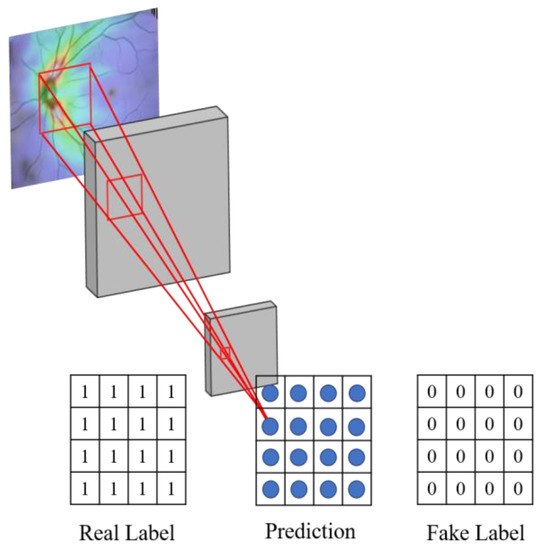
Figure 13. Schematic diagram of the receptive field of the discriminator.

The reason for using the convolution operation in the last layer is to allow the feature matrix produced by the discriminator to be traced back to a specific region of the original image.

In order to improve the performance of the discriminator, the mean-square error (MSE) is used as the loss function for our Markovian Discriminator. The MSE can measure the average between the predicted value and the real value; the smaller the value, the higher the similarity.

Suppose the label of the real image is z, and the label of the generated image is $\overline{z}$. In order to measure the data distribution output by the real image and the generated image through the discriminator, we denote the Euclidean distance between the score obtained by feeding the real image x to the discriminator and the real image label z as D_real, defined as Equation (6). We also denote the Euclidean distance between the score obtained by feeding the generated image y to the discriminator and the generated image label $\overline{z}$ as D_fack, defined as Equation (7).

$$D_{real}=\frac{1}{mn}{\sum }_{i=1}^n{\sum }_{j=1}^m{\left(z^{ij}-x^{ij}\right)}^2,$$

(6)

$$D_{fake}=\frac{1}{mn}{\sum }_{i=1}^n{\sum }_{j=1}^m{\left({\overline{z}}^{ij}-y^{ij}\right)}^2,$$

(7)

where m and n are the size of the image length and width.

This method allows the data distribution in the generated images to be closer to real OCT images. The loss of discriminator is defined as:

$$DiscriminatorLoss=\left(D_{real}+D_{fake}\right)\times 0.5,$$

(8)

3.4. Glaucoma Classification with Incremental Learning

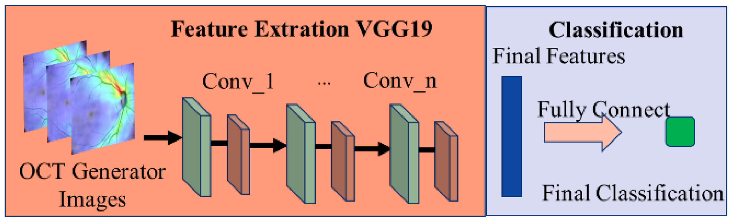
This paper uses a VGG19-based model (shown in Figure 14) [27] to classify the presence of glaucoma in OCT images. VGG mainly uses the idea of adding convolutional layers to improve the classification ability of the model.

Figure 14. Schematic diagram of the glaucoma classification model.

However, due to different equipment and settings in different fields, the captured image quality is also different, which will reduce the accuracy of the classifier. Traditionally, this problem has been solved by adding new images obtained from new fields and retraining the classifier to improve accuracy. However, this has a cost for retraining the model. Therefore, this paper uses the transfer learning concept [28] to design a classification model architecture for incremental learning.

The proposed transfer learning method will manually re-judge and label the results of the glaucoma classification model by ophthalmologists and use these images as a training set for the incremental model so that the model can learn the difference between the old image and the new image. Therefore, the initially learned information about judging the features of glaucoma can be transferred to the new classification model, improving the model’s identification accuracy in the new field in a short time. Figure 15 shows the schematic diagram of the transfer learning process.

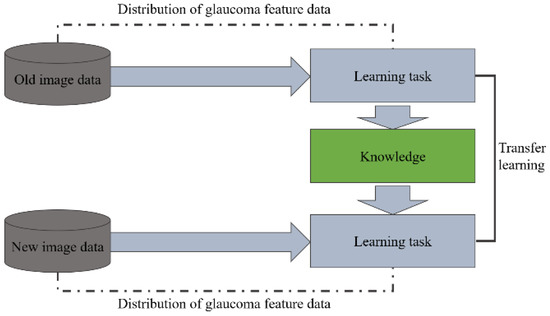
Figure 15. Schematic diagram of the transfer learning process.

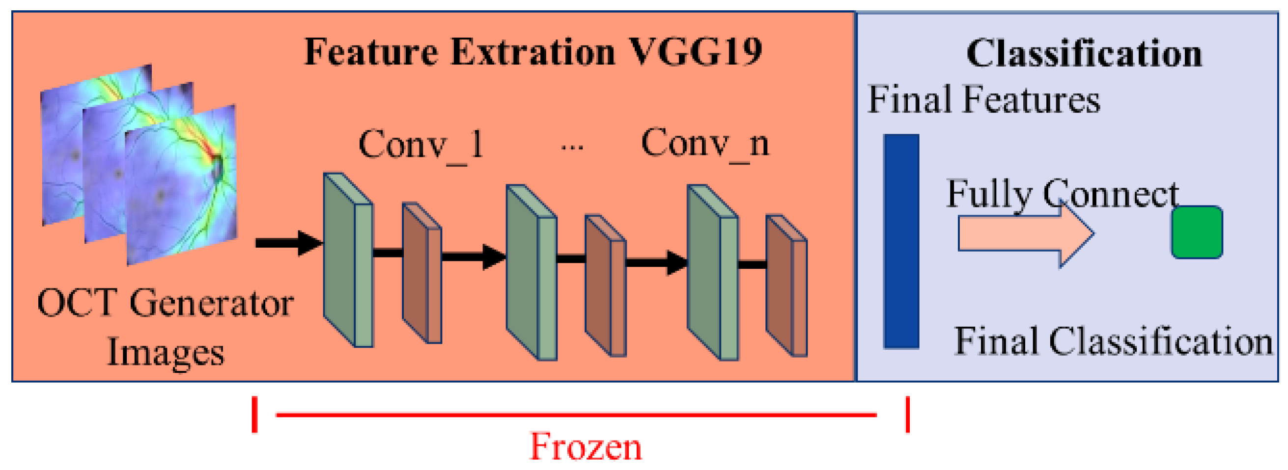
We have observed from experiments that the reason for the decline in classifier accuracy is the result of model output weight deviation. Therefore, as shown in Figure 16, the transfer learning method is used for incremental learning. We freeze the feature extraction part of the initial model and only train the classifier for bias correction to improve the model’s classification accuracy.

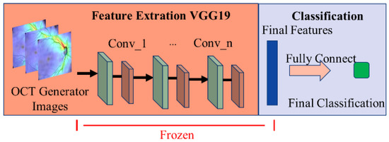
Figure 16. Schematic diagram of the incremental method for glaucoma classification model training.

We use binary cross-entropy (BCE) to evaluate the performance of the classifier for identifying glaucoma, where a larger value indicates a higher probability of glaucoma. The BCE is defined as:

$$BCE\left(O,T\right)=-\frac{1}{N}{\sum }_{i=1}^N{T}_i\cdot \mathit{log}\left(O_i\right)+\left(1-T_i\right)\cdot \mathit{log}\left(1-O_i\right),$$

(9)

where O is the label predicted by the model, T is the real label, and N is the amount of data in each batch.

The proposed system uses the predicted probability (between 0 and 1) output by the classification model as the final model prediction O with a threshold of 0.5. The larger the value, the higher the probability of the image being glaucoma. We compare the result judged by the classifier with the real label T to correct the model’s parameters.

4. Results and Discussion

This section presents the experimental results of our proposed glaucoma detection system, including the effect of the OCT generator and glaucoma classifier. A comparison with the results of other generative methods is also presented. Finally, we demonstrate the effectiveness of implementing incremental learning in a new field.

4.1. Generation of OCT Images

4.1.1. Dataset and Experimental Environment for OCT Generation

The fundus and OCT images used in the experiment were obtained from the Department of Glaucoma, Chang Gung Memorial Hospital. As shown in Table 1, the total number of experimental images is 441, and we randomly divide them into 200 for training and 201 for testing at 1:1.

Table 1. Quantity of the experimental images.

	Quantity	Training	Testing
Fundus	441	220	221
OCT	441	220	221

The fundus and OCT images were captured by the DRI OCT Triton (Swept Source OCT, Topcon, Oakland, NJ, USA). In order to ensure the correctness of labeling, all images in the experiment were judged by two glaucoma physicians of Chang Gung Memorial Hospital and labeled as glaucoma or not. Before model training, ophthalmologists assist in identifying and labeling fundus and OCT images. When testing, ophthalmologists also review the classification results of the system. The fundus image size is 2576 × 1934, and the OCT image size is 903 × 663.

The hardware used in the experiment is: AMD Ryzen 7 8-core CPU, 32GB DRAM, and NVidia GeForce RTX 2080 Ti graphics card. The software environment and tools include Microsoft Windows 10, Python, Pytorch, and OpenCV.

In this experiment, when training the generator and the discriminator, the relevant parameters are set to 2500 training iterations, the batch size is 8, the optimizer is RMSprop, and the learning rate is 1 × 10⁻³.

4.1.2. Evaluation Criteria for Generative Models

To evaluate the quality of the generated OCT images, we adopt the Peak Signal-to-Noise Ratio (PSNR) [29], Structural Similarity Index (SSIM) [30], Multi-Scale Structural Similarity Index (MS-SSIM), and Cosine Similarity (COSIN) [31] as the evaluation criteria. PSNR is the ratio between the maximum value of the measured signal and the number of noises which affect the image. The Peak Signal-to-Noise Ratio between the real OCT image x and generated OCT image y is defined as

$$PSNR\left(x,y\right)=10\cdot {log}_{10}({255}^2/MSE(x,y\left)\right),$$

(10)

where MSE(x,y) denotes the mean square error of the real OCT image x and generated OCT image y, i.e.,

$$MSE(x,y)=\frac{1}{MN}{\sum }_{i=1}^N{\sum }_{j=1}^M{\left(x^{ij}-y^{ij}\right)}^2,$$

(11)

where M and N represent the width and height of the image, respectively. Here, the contrast enhancement method with a smaller MSE value and larger PSNR value significantly outperforms other contrast enhancement methods.

The Structural Similarity Index between the real OCT image x and generated OCT image y is defined as

$$SSIM=l\left(x,y\right)\cdot c\left(x,y\right)\cdot s\left(x,y\right),$$

(12)

where l(x,y), c(x,y), and s(x,y) represent the image brightness, contrast, and structure defined in Equations (2)–(4).

The Multi-Scale Structural Similarity Index between the real OCT image x and generated OCT image y is defined in Equation (1).

The Cosine Similarity between the real OCT image x and generated OCT image y is defined as

$$\mathit{COSIN}\left(x,y\right)=\frac{x\cdot y}{‖x‖\times ‖y‖}=\frac{{\sum }_{i=1}^n{x}_i\times y_i}{\sqrt{{\sum }_{i=1}^n{x}_i^2}\times \sqrt{{\sum }_{i=1}^n{y}_i^2}},$$

(13)

where the real and generated OCT images are transposed into the vector space. The similarity between real and generated OCT image pixels is obtained from the corresponding feature vectors. The cosine, i.e., the angle between the two vectors, is closer to 1. The smaller the angle, the more similar the generated OCT image y is to the real OCT image x.

4.1.3. Comparison with Different Generative Models

Image quality measurement methods can be roughly divided into three categories, including pixel distance-based, correlation-based, and mean square error-based [32]. To verify the effectiveness of the proposed image generation model, we compared it to Autoencoder [33], DCGAN [34], U-Net [35], and other generative models. Figure 17 presents the results of our proposed OCR generation model and other models.

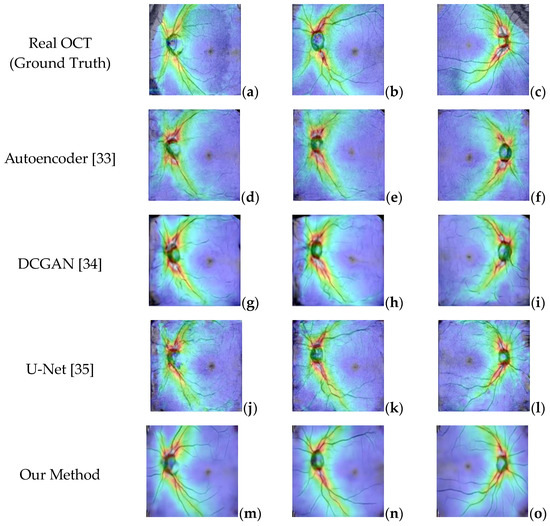
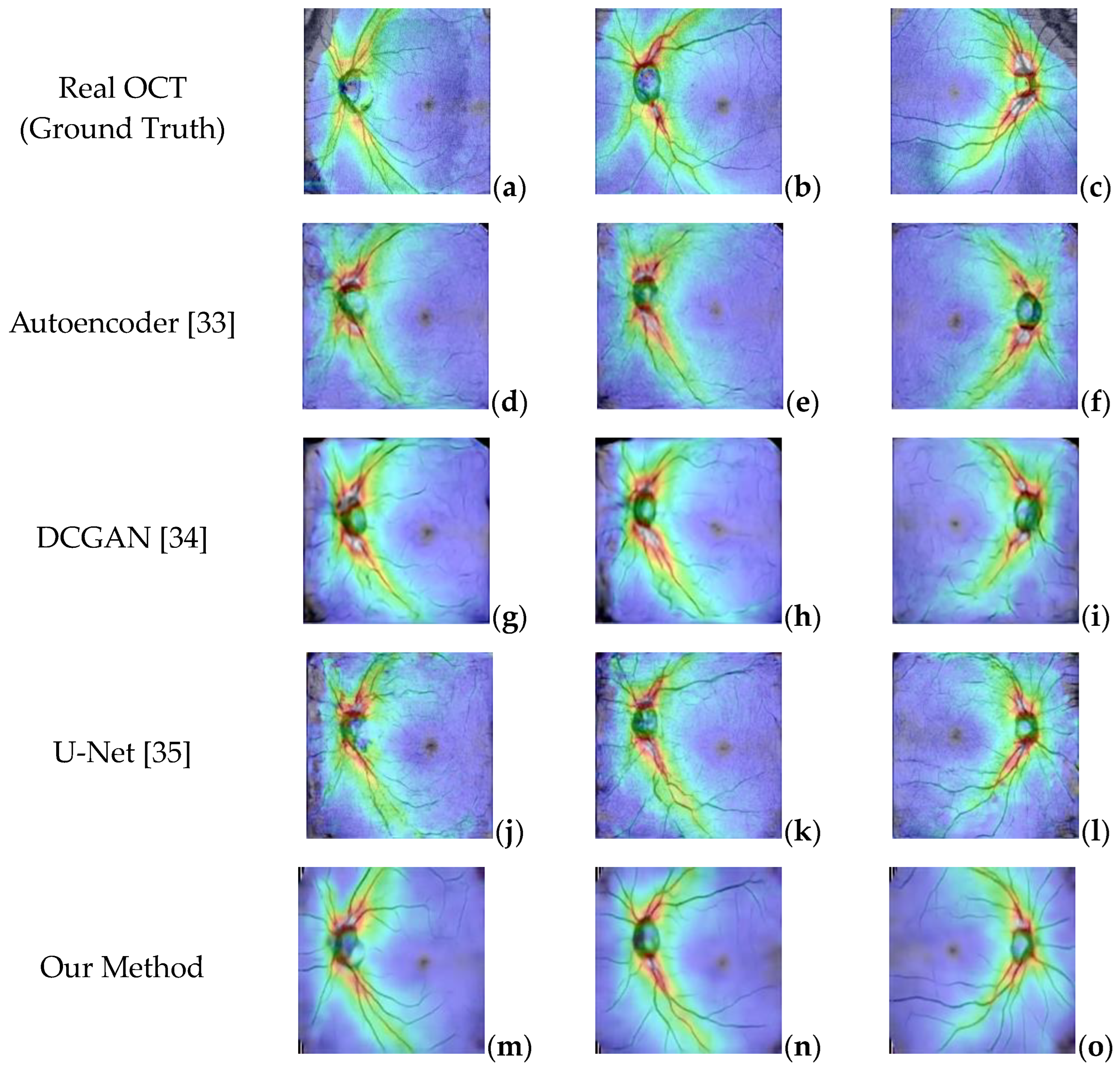
Figure 17. (a–c) Real OCT images. (d–f) Generated OCT by Autoencoder. (g–i) Generated by DCGAN. (j–l) Generated by Unet. (m–o) Generated by the proposed method.

The experimental results in Figure 17 show that although the Autoencoder and DCGAN models can generate images similar to real OCT images, they cannot replicate the blood vessels and other small details in the image. Similarly, the U-Net model can capture more detail in the images but is still not ideal because it cannot handle the branches in the blood vessels. In contrast, the images generated using the proposed OCT generative model are smoother, more realistic, and more similar to real images.

To evaluate the OCT generation effect of different generative models, we use the generated OCT images and the original real OCT images from the test set of 221 fundus images and use Equations (10)–(13) to calculate PSNR, MSE, SSIM, and COSIN for each generated OCT image and the original corresponding OCT image, and finally expressed the results as the average value. Table 2 presents the performance comparison of various generative models under different evaluation criteria. The proposed method achieves the highest performance compared to other methods.

Table 2. Comparison of images generated by different architectures.

	SSIM	PSNR	MS-SSIM	COSIN
Autoencoder [33]	22.2%	65.67%	24.0%	97.7%
DCGAN [34]	22.7%	64.72%	24.7%	97.3%
U-Net [35]	21.3%	65.54%	22.4%	97.6%
Our method	27.2%	65.78%	28.7%	97.8%

Because the optic disc area on an OCT scan allows doctors to identify optic atrophy and determine macular thickness, it plays an essential role in glaucoma screening. Therefore, to further evaluate the effectiveness of the proposed generator, we randomly capture ten optic disc regions of size 130 × 130 from the generated OCT images. Figure 18 shows two OCT images generated by different methods. The images in the table are generated and cropped to the optic disc area, and the disc size is 130 × 130.

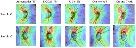
Figure 18. The generated results of various methods.

Table 3 lists the similarity measures of the optic disc region between generated and real OCT images. Obviously, the proposed method achieves better generative results than other architectures.

Table 3. Similarity of the optic disc area between the generated and real OCT images.

	SSIM	PSNR	MS-SSIM	COSIN
Autoencoder [33]	15.4%	65.16%	16.4%	98.1%
DCGAN [34]	17.8%	64.69%	18.9%	97.7%
U-Net [35]	19.3%	65.63%	19.1%	98.2%
Our method	22.4%	66.24%	21.8%	98.5%

4.2. Classification of Glaucoma

4.2.1. Dataset and Experimental Setting for Glaucoma Classification

The dataset used for glaucoma classification consists of generated OCT images and real OCT images. Although the generated images are similar to real OCT scans, there are still noticeable differences, and the generated images tend to be smoother, as shown in Figure 18. In order to improve the robustness of the image classification model, we performed transfer learning when training the glaucoma classification model.

We first train the glaucoma classification model using the generated OCT images and then use the real OCT images for the second training. In Table 4, we divide the images into 75% as the training set and 25% as the test set for the experiment.

Table 4. Dataset of generated OCT images.

Dataset		Generated OCT	Real OCT
Training set	Glaucoma	208	208
	Normal	115	115
Testing set	Glaucoma	75	75
	Normal	32	32

When training the glaucoma classifier, the VGG19 architecture is used as the classifier. The relevant parameters are set as follows: 50 training iterations, the batch size is 16, the optimizer uses Adam, and the learning rate is 2 × 10⁻⁵.

4.2.2. Evaluation Criteria for Glaucoma Classification Models

To evaluate the performance of the proposed classifier, we adopt evaluation criteria, including precision, sensitivity, specificity, and accuracy. The equations for these metrics are defined below:

$$Precision=\frac{TP}{TP+FP},$$

(14)

$$Sensitivity=\frac{TP}{TP+FN},$$

(15)

$$Specificity=\frac{TN}{TN+FP},$$

(16)

$$Accuracy=\frac{TP+FN}{TP+TN+FP+FN},$$

(17)

where TP represents the number of glaucoma cases that are classified as glaucoma correctly, TN represents the number of normal cases classified as normal, FP denotes the number of normal cases misclassified as glaucoma, and FN denotes the number of glaucoma cases misclassified as normal.

In general, precision indicates the general performance of the classifier [36]. Sensitivity shows the ability to detect the correct pixels accurately [10]. Specificity means the ability to accurately detect pixels that are not part of the region [10]. Accuracy indicates how accurately the ground truths match the segmented result. The improved accuracy shows a better outcome of the proposed algorithm.

4.2.3. Comparison with Different Classification Models

The primary purpose of the glaucoma classification model is to identify whether there is glaucoma from the generated OCT images. To evaluate the performance of the VGG19 classifier for identifying glaucoma from OCT images, we trained the classifier on real OCT images and generated OCT images separately.

As shown in Table 5, we achieved 75.70% and 84.11% accuracy when training the classification model using only generated or real OCT images, respectively. These results suggest that training with only generated images will yield poor results.

Table 5. Training results of the classification model.

	Trained by Real OCT	Train by Generated OCT	Trained by Transfer Learning
Precision	86.25%	78.82%	85.19%
Sensitivity	92.00%	89.33%	92.00%
Specificity	65.62%	43.75%	62.50%
Accuracy	84.11%	75.70%	83.17%

Furthermore, using the proposed method (shown in Figure 15), the classification model is first trained using the generated images and then retrained using real OCT images via transfer learning. From the experimental results shown in the rightmost column of Table 5, the performance of the classifier is greatly improved, which indicates that the proposed transfer learning method is indeed feasible.

In order to improve the accuracy of the VGG 19 network for glaucoma classification, we first train the classifier by generated images so that the VGG 19 network can learn the features of the generated images, and then the retrain classifier with real OCT images to correct the bias accumulated during the first training.

This paper also compares the performance of our proposed transfer learning method with RestNet-18 and DenseNet-20 for glaucoma classification. As shown in Table 6, the transfer learning method has better classification performance.

Table 6. Comparison with other methods.

	ResNet-18	DenseNet-20	The Proposed Transfer Learning
Precision	79.76%	77.42%	85.19%
Sensitivity	89.33%	96.00%	92.00%
Specificity	46.88%	34.38%	62.50%
Accuracy	76.63%	77.57%	83.17%

4.3. Increamental Training for Glaucoma Classifier

4.3.1. Dataset and Experimental Setting for Incremental Training

In reality, due to different equipment settings in various fields, the classification accuracy will decrease. This phenomenon can use incremental training to allow the classifier to quickly learn the differences between old and new images and quickly transfer glaucoma features to the new classification model.

Table 7 shows the number of image data sets used in this incremental training experiment. These images are provided by the Glaucoma Department of Chang Gung Memorial Hospital, and the images are all fundus images. In this experiment, all fundus images were also labeled by glaucoma physicians for glaucoma.

Table 7. Dataset of extra generated OCT images.

Dataset	# of Images
Training set	Glaucoma	232
	Normal	92
Testing set	Glaucoma	88
	Normal	21

Furthermore, the experiment aims to demonstrate the effectiveness of our proposed model by using a new dataset. We feed additional fundus images into the generator model to generate new OCT images and use the 433 generated images at a 3:1 ratio for training and testing, as shown in Table 8.

Table 8. Results before and after incremental training.

	Trained by Initial Model	Trained by Incremental Model
Precision	71.70%	85.00%
Sensitivity	95.00%	85.00%
Specificity	11.76%	64.71%
Accuracy	70.17%	78.94%

In this experiment, the relevant parameters for incremental training are: the number of the epoch is set to 50, the batch size is set to 8, the optimizer uses Adam, and the learning rate is set to 10⁻⁵.

4.3.2. Comparison of Whether to Use Incremental Training

To verify the effectiveness of the proposed incremental training method, we use the additional image data in Table 8 to train the glaucoma classifier. We compare the classification results with and without incremental training, as shown in Table 8. The classifier using the incremental training method has a better classification accuracy.

5. Conclusions

Glaucoma is an eye disease caused by damage to the optic nerve. Screening for glaucoma is often limited to large hospitals because of the difficulty in identifying early symptoms and the unaffordability of expensive OCT equipment in community or small-town eye clinics.

In this paper, we propose a GAN model that can generate realistic OCT images using only fundus images, which doctors can refer to in order to judge whether patients need further screening, thereby increasing the chances of early detection and treatment.

Experimental results show that the cosine similarity between the OCT images generated by the proposed method and real OCT images is 97.8%. The experiments compared with other methods also show that the performance of the proposed method is significantly better than that achieved using autoencoders, DCGAN, and U-Net. Moreover, using the proposed transfer learning method, the accuracy of the classification model is about 83.17%. Furthermore, using the incremental training method also increased the accuracy of glaucoma identification to approximately 78.94%, which is 8.77% higher than the 70.17% without incremental learning techniques, which shows that the proposed method can effectively improve the accuracy of glaucoma classification in different fields.

References

- Tham, Y.C.; Li, X.; Wong, T.Y.; Quigley, H.A.; Aung, T.; Cheng, C.Y. Global prevalence of glaucoma and projections of glaucoma burden through 2040. Ophthalmology 2014, 121, 2081–2090. [Google Scholar] [CrossRef] [PubMed]
- Anindita, S.; Agus, H. Automatic glaucoma detection based on the type of features used: A review. J. Theor. Appl. Inf. Technol. 2015, 72, 366–375. [Google Scholar]
- Roslin, M.; Sumathi, S. Glaucoma screening by the detection of blood vessels and optic cup to disc ratio. In Proceedings of the IEEE International Conference on communication and Signal Processing, Melmaruvathur, India, 6–8 April 2016. [Google Scholar]
- Zheng, C.; Johnson, T.; Garg, A.; Boland, M.V. Artificial intelligence in glaucoma. Curr. Opin. Ophthalmol. 2019, 30, 97–103. [Google Scholar] [CrossRef] [PubMed]
- Schmitt, J.M. Optical coherence tomography (OCT): A review. IEEE J. Sel. Top. Quantum Electron. 1999, 5, 1205–1215. [Google Scholar] [CrossRef]
- Serranho, P.; Morgado, A.; Bernardes, R. Optical coherence tomography: A concept review. In Biological and Medical Physics, Biomedical Engineering; Springer Science + Business Media: Berlin, Germany, 2012; pp. 139–156. [Google Scholar]
- Heidari, A.; Toumaj, S.; Navimipour, N.J.; Unal, M. A privacy-aware method for COVID-19 detection in chest CT images using lightweight deep conventional neural network and blockchain. Comput. Biol. Med. 2022, 145, 105461. [Google Scholar] [CrossRef]
- Heidari, A.; Jafari Navimipour, N.; Unal, M.; Toumaj, S. Machine learning applications for COVID-19 outbreak management. Neural Comput. Appl. 2022, 34, 15313–15348. [Google Scholar] [CrossRef] [PubMed]
- Suryani, A.I.; Chang, C.W.; Feng, Y.F.; Lin, T.K.; Lin, C.W.; Cheng, J.C.; Chang, C.Y. Lung Tumor Localization and Visualization in Chest X-Ray Images Using Deep Fusion Network and Class Activation Mapping. IEEE Access 2022, 10, 124448–124463. [Google Scholar] [CrossRef]
- Shen, L.; Margolies, L.R.; Rothstein, J.H.; Fluder, E.; McBride, R.; Sieh, W. Deep Learning to Improve Breast Cancer Detection on Screening Mammography. Sci. Rep 2019, 9, 12495. [Google Scholar] [CrossRef]
- Abdullah, F.; Imtiaz, R.; Madni, H.A.; Khan, H.A.; Khan, T.M.; Khan, M.A.; Naqvi, S.S. A Review on Glaucoma Disease Detection Using Computerized Techniques. IEEE Access 2021, 9, 37311–37333. [Google Scholar] [CrossRef]
- Thakur, N.; Juneja, M. Survey on segmentation and classification approaches of optic cup and optic disc for diagnosis of glaucoma. Biomed. Signal Process. Control. 2018, 42, 162–189. [Google Scholar] [CrossRef]
- Maheshwari, S.; Pachori, R.; Acharya, U. Automated diagnosis of glaucoma using empirical wavelet transform and cor-rentropy features extracted from fundus images. IEEE J. Biomed. Health Inf. 2016, 21, 803–813. [Google Scholar] [CrossRef] [PubMed]
- Acharya, U.R.; Bhat, S.; Koh, J.E.; Bhandary, S.V.; Adeli, H. A novel algorithm to detect glaucoma risk using texton and local configuration pattern features ex-tracted from fundus images. Comput. Biol. Med. 2017, 88, 72–83. [Google Scholar] [CrossRef] [PubMed]
- Kankanala, M.; Kubakaddi, S. Automatic segmentation of optic disc using modified multi-level thresholding. In Proceedings of the 2014 IEEE International Symposium on Signal Processing and Information Technology (ISSPIT), Noida, India, 15–17 December 2014; pp. 000125–000130. [Google Scholar]
- Juneja, M.; Singh, S.; Agarwal, N.; Bali, S.; Gupta, S.; Thakur, N.; Jindal, P. Automated detection of glaucoma using deep learning convolution network (G-net). Multimedia Tools Appl. 2019, 79, 15531–15553. [Google Scholar] [CrossRef]
- Lee, S.; An, G.H.; Kang, S.J. Generative adversarial networks. Adv. Neural Inf. Pro-Cessing Syst. 2014, 2018, 2672–2680. [Google Scholar]
- Bisneto, T.R.; de Carvalho Filho, A.O.; Magalhães, D.M. Generative adversarial network and texture features applied to automatic glaucoma detection. Appl. Soft Comput. 2020, 90, 106165. [Google Scholar] [CrossRef]
- Bisneto, T.R.; de Carvalho Filho, A.O.; Magalhães, D.M. Accuracy of Using Generative Adversarial Networks for Glaucoma Detection: Systematic Review and Bibliometric Analysis. J. Med. Internet Res. 2021, 23, e27414. [Google Scholar] [CrossRef]
- Thrun, S.; Pratt, L. Learning to Learn; Kluwer Academic Publishers: Amsterdam, The Netherlands, 1998. [Google Scholar]
- Caruana, R. Multitask Learning. Mach. Learn. 1997, 28, 41–75. [Google Scholar] [CrossRef]
- Gurbuz, A.C.; McClellan, J.H.; Scott, W.R., Jr. Use of the Hough Transformation to Detect Lines and Curves in Pictures, Comm. ACM 1972, 15, 11–15. [Google Scholar]
- Reza, A. Realization of the Contrast Limited Adaptive Histogram Equalization (CLAHE) for Real-Time Image Enhancement. J. VLSI Signal Process. 2004, 38, 35–44. [Google Scholar] [CrossRef]
- LeCun, Y.; Boser, B.; Denker, J.; Henderson, R.E.; Howard, W.; Hubbard; Jackel, L.D. Backpropagation applied to handwritten zip code recognition. Neural Comput. 1989, 1, 541–551. [Google Scholar] [CrossRef]
- Wang, X.; Girshick, R.; Gupta, A.; He, K. Non-local neural networks. In Proceedings of the IEEE Conference on Computer Vision and Pattern Recognition (CVPR), Salt Lake City, UT, USA, 18–22 June 2018; pp. 7794–7803. [Google Scholar]
- Isola, P.; Zhu, J.-Y.; Zhou, T.; Efros, A.A. Image-to-image translation with conditional adversarial networks. In Proceedings of the IEEE Conference on Computer Vision and Pattern Recognition (CVPR), Honolulu, HI, USA, 21–26 July 2017; pp. 1125–1134. [Google Scholar]
- Wang, Z.; Simoncelli, E.; Bovik, A.C. Multiscale structural similarity for image quality assessment. In Proceedings of the Thrity-Seventh Asilomar Conference on Signals, Systems & Computers, Pacific Grove, CA, USA, 9–12 November 2003; pp. 1398–1402. [Google Scholar]
- Simonyan, K.; Zisserman, A. Very deep convolutional networks for large-scale image recognition, arXiv preprint. arXiv 2014, 1409, 1556. [Google Scholar]
- Hore, A.; Ziou, D. Image quality metrics: PSNR vs. SSIM. In Proceedings of the 2010 20th International Conference on Pattern Recognition, Istanbul, Turkey, 23–26 August 2010; pp. 2366–2369. [Google Scholar]
- Wang, Z.; Bovik, A.; Sheikh, H.; Simoncelli, E.P. Image quality assessment: From error visibility to structural similarity. IEEE Trans. Image Process. 2004, 13, 600–612. [Google Scholar] [CrossRef] [PubMed]
- Nguyen, H.V.; Bai, L. Cosine similarity metric learning for face verification. In Proceedings of the Asian Conference on Computer Vision, Queenstown, New Zealand, 8–12 November 2010; pp. 709–720. [Google Scholar]
- Shih, F.Y. Image Processing and Pattern Recognition: Fundamentals and Techniques; Wiley: Hoboken, NJ, USA, 2010. [Google Scholar]
- Boesen, A.; Larsen, L.; Sonderby, S. Generating Faces with Torch. 2015. Available online: www.torch.ch/blog/2015/11/13/gan.html (accessed on 20 January 2021).
- Li, J.; Jia, J.; Xu, D. Unsupervised representation learning of image-based plant disease with deep convolutional generative adversarial networks. In Proceedings of the 2018 37th Chinese Control Conference (CCC), Wuhan, China, 25–27 July 2018; pp. 9159–9163. [Google Scholar]
- Ronneberger, O.; Fischer, P.; Brox, T. U-net: Convolutional networks for biomedical image segmentation. In Proceedings of the International Conference on Medical Image Computing and Computer-Assisted Intervention, Munich, Germany, 5–9 October 2015; pp. 234–241. [Google Scholar]
- Bernabe, O.; Acevedo, E.; Acevedo, A.; Carreno, R.; Gomez, S. Classification of eye diseases in fundus images. IEEE Eng. Med. Biol. Soc. Sect. 2021, 9, 267–276. [Google Scholar] [CrossRef]
Disclaimer/Publisher’s Note: The statements, opinions and data contained in all publications are solely those of the individual author(s) and contributor(s) and not of MDPI and/or the editor(s). MDPI and/or the editor(s) disclaim responsibility for any injury to people or property resulting from any ideas, methods, instructions or products referred to in the content. |
© 2023 by the authors. Licensee MDPI, Basel, Switzerland. This article is an open access article distributed under the terms and conditions of the Creative Commons Attribution (CC BY) license (https://creativecommons.org/licenses/by/4.0/).