Featured Application
The method proposed can be used for target reachable zone prediction of boosting gliding vehicle.
Abstract
This paper presents an effective method for the fast prediction of the target reachable zone of a boosting gliding vehicle in the gliding phase. Firstly, a six-point method is proposed for the rapid determination of the reachable zone and the feasible discrimination of the target. The method chooses six boundary points with notable features to characterize the reachable zone and considerably reduces the computational consumption. Furthermore, taking into account the need for a rapid launch and safety against unexpected events during the gliding phase, a database method for the prediction of the reachable zone is presented, which builds the database with time nodes and six boundary points and employs interpolation methods to calculate the reachable zone. The results suggest that online planning by the database method has significant potential for predicting the target reachable zone. The accuracy error is less than 1%, and the computational efficiency is increased by 90% when compared to the six-point approach.
1. Introduction
A boosting gliding vehicle is a special kind of vehicle that is propelled by a booster rocket to a specific altitude and speed before re-entering the atmosphere and gliding back to earth. It flies at a maximum altitude of 200 km or less and at a speed of over 5 Ma. Furthermore, the atmosphere has a noticeable impact on the entry gliding process, which is highly nonlinear, strongly coupled to the environment, and subject to complicated constraints. This presents a very serious challenge to trajectory planning. In terms of practical applications, the requirement for the rapid launch of boosting gliding vehicles is raised by ground commanders. The range capabilities of the vehicle and its ability to hit the target must be known by the commanders when a striking target has been selected. The entire decision-making process is typically completed in a short time. In addition, it is possible that the gliding vehicle will encounter unusual occurrences or unexpected faults [1,2]. In these circumstances, the vehicle should be able to operate autonomously and make decisions such as abandoning the preplanned mission and immediately implementing safety measures. It is necessary to quickly predict a new target that can be reached based on the current state and to make a reasonable selection of target points, which provide basic information for the ground commander to develop countermeasures. The main objective is to study the calculation of the vehicle’s reachable zone during the gliding phase to improve the computational efficiency and to provide the potential for online replanning, thus achieving improved survivability, operational effectiveness, and safety of the vehicle.
In general, there are two main trajectory prediction methods for a gliding vehicle: the analytical method [3,4,5,6,7,8,9] and the numerical method [10,11,12,13,14,15]. The analytical method is an intuitive method to predict the trajectory of a hypersonic vehicle. In the process of prediction, the analytical expression of the trajectory is usually obtained by solving the dynamics model according to the current state. However, due to the complex coupling relationship, only first- or second-order approximate solutions can be obtained by reasonable simplification. Zhang et al. [3] developed high-precision analytical solutions for 3-dimensional (3-D) hypersonic gliding trajectory over the rotating and spherical Earth using the regular perturbation method. Aiming at the special gliding problem where the gliding speed is close to the first cosmic speed, Yu et al. [4] planned a drag acceleration profile and derived the analytical solution of a three-dimensional special gliding trajectory by properly simplifying the nonlinear equations of motion. The numerical method firstly creates the control input and then predicts the trajectory by using the integral method. The designed control input can be a bank angle or a generalized flight profile characterizing the vehicle’s motion, such as a drag acceleration–velocity (D-V) profile [11] or a drag acceleration–lateral lift-to-drag ratio–energy () profile [12]. More enticingly, the numerical method can be employed for the trajectory planning of complicated flight missions that take multiple waypoints and no-fly zone constraints into consideration because of its algorithmic robustness and adaptability to path constraints and terminal constraints. Zhang et al. [13] proposed a new entry trajectory generation method for hypersonic glide vehicles based on a three-dimensional acceleration profile which meets range requirements while considering waypoint and no-fly zone constraints.
The reachable zone [16,17] is an important indicator for evaluating the coverage range and flight capability of a boosting gliding vehicle. The results of the reachable zone calculation and the perception of the current vehicle status can also be used by the vehicle to decide whether to switch to a new target location or a new tracking profile, as well as whether to implement a new safe disposal plan autonomously or with the help of ground commanders. This can increase the autonomy and safety of the vehicle. The methods for the calculation of the reachable zone have been extensively studied by many scholars at present, mainly the constant bank angle method [18,19], the optimization method [20,21,22,23], and the profile design method [24,25]. The constant bank angle method, which is frequently employed in engineering, is simple, reliable, and rapid, although it contains certain errors when compared to the actual reachable zone. The optimization approach is the most precise solution method now accessible, but the pace of the solution is very slow, necessitating additional study to fulfil the requirements of online planning. Arslantas et al. [20] proposed an algorithm for the approximation of nonconvex reachable sets by using optimal control. The proposed method computes approximated reachable sets and the attainable safe landing zone with information about propellant consumption and time and is applied to a generic Moon landing mission. Zhao et al. [22] proposed a method based on the analytical homotopic approach to analyze the flight capability of a Mars atmospheric entry vehicle. Based on the solutions to optimization problems, the reachable longitudinal area can be determined iteratively by setting a proper continuation parameter. The reachable zone calculated by the profile design method is easy and practical. Firstly, the entry process constraints are translated into a generalized flight profile, and a flight corridor is formed. Then, entry-designed profiles are planned along the corridor boundaries to form the maximum and minimum range profiles as well as all the feasible profiles. Finally, the corresponding trajectory endpoints of each profile are connected to obtain the reachable zones. He et al. [25] proposed a new landing footprint generation algorithm that considers multiple uncertainty effects based on an improved 3D acceleration profile planning method.
In short, there are several gaps in the current works on the reachable zone of boosting gliding vehicles, such as low computational efficiency and poor adaptability. What is more, the current literature is not conducive to the study of online prediction for the reachable zone because of low computational efficiency. Aimed at solving the above problems, this paper proposes a fast prediction method for the target reachable zone of a boosting gliding vehicle based on a database. The database of the target reachable zone can be built in advance using the standard trajectory that was previously designed. In the process of the gliding phase, when the vehicle encounters an emergency, the commander can quickly predict the reachable zone at the current moment based on the database method, which provides theoretical support for the online trajectory replanning of the gliding vehicle. The structure of this paper is as follows: Section 2 establishes the motion formulation and the constraints for the boosting gliding vehicle; the preliminary D-V profile method is introduced in Section 3; in Section 4, the effective reachable zone prediction method is proposed; the simulated examples demonstrating the validity and accuracy of the reachable zone prediction method are detailed in Section 5. We conclude this paper in Section 6.
2. Problem Formulation
This section first provides a primal motion model for the trajectory-planning problem. In the gliding phase, the entry is treated as a constant mass point without any power over the spherical rotational Earth, which is affected by gravitational and aerodynamic forces. Therefore, many complex constraints should be considered during hypersonic glider flight, such as aero heating, dynamic pressure, load factor, and other state constraints.
2.1. Equations of Motion
The equations of motion over the rotating spherical Earth for the vehicle’s gliding phase are established as follows [7]:
where is the velocity relative to the Earth, is the flight path angle, is the bank angle, is the heading angle at which a vehicle’s velocity is projected onto a local horizontal plane concerning the local north, clockwise is the positive direction, is the longitude, is the latitude, and is the radius from Earth’s center to the vehicle center of mass. is the mass of the vehicle, and is the reference area. is the angular velocity of the Earth’s rotation, and are the component of the Earth’s gravitational acceleration in the direction of the geocentric radius vector and the angular velocity of the Earth’s rotation, respectively. , , and are the lift coefficient, drag coefficient, and lateral force coefficient, respectively. is the atmospheric density.
2.2. Gliding Phase Constraints
In general, the three fundamental forms of path constraint that the gliding phase trajectory planning should satisfy are normally the heating rate , dynamic pressure , and load factor . Path constraints are given by [14]:
where is a heating rate constant relative to the material of the head of the vehicle; k = 5 × 10⁻⁵; , , and are the maximum heating rate, dynamic pressure, and load factor respectively; is the gravitational acceleration at sea level; and D and L are the drag and lift accelerations, respectively.
The following control constraints on the amplitude and rate of the angle of attack (AoA) and bank angle, which are likewise handled as one part of the path constraints, should also be satisfied by the trajectory planning during the gliding phase:
where , , , and are the minimum and maximum AoA and bank angle, respectively. and are the maximum AoA rate and bank angle rate, respectively.
The altitude and speed of the vehicle at the end of the glide phase are regarded as the terminal constraints:
where the superscript means the terminal constraint.
3. D-V Profile Method Preliminary
The basic concepts of the drag acceleration–velocity (D-V) profile method method (see Appendix A for full trans) are first presented in this section, and then we derive the profile tracking guidance law and the bank reversal logic, which serve as the theoretical background for the ongoing reachable zone prediction methods.
3.1. Profile Tracking Guidance Law
As illustrated in Figure 1, there are two major boundary constraints for the D-V profile design. On one hand, the upper black, thick, solid line is the consequence of the maximum heating rate, dynamic pressure, and load factor constraints combined as a D-V profile upper boundary constraint. That is a hard constraint, and to avoid serious safety problems including excessive thermal ablation of the vehicle, structural damage, and control failure, the D-V profile can only be designed to travel below this boundary. On the other hand, the lower black, thick, solid line, also described as the lower boundary, which is constrained by the quasi-equilibrium gliding condition, is a soft constraint that the vehicle is free to ignore and along which a greater range in the gliding phase can be obtained. The upper and lower boundaries are combined to give a range of profile designs known as flight corridors. The D-V profile is designed as a three-fold line in the drag acceleration corridor indicated by the constraints. The red line represents the profile to be designed. As the design profile moves upwards, it means increases, and the range of the vehicle will gradually decrease. In contrast, as the design profile moves downwards, the range of the vehicle will gradually increase.
Figure 1.
The D-V designed profile schematic.
When the D-V profile is designed in the form of a three-fold line, as in Figure 1, a quadratic (or sub-quadratic) curve of the designed D-V profile is uniformly expressed as follows:
The whole corresponding range for this designed D-V profile is:
Once the reference D-V profile is determined, the standard lift-to-drag ratio of the vehicle along that designed profile can be found [26,27], denoted as .
The vehicle will also be guided to the predetermined target by a longitudinal trajectory tracking controller, and the required lift-to-drag ratio and its small increment will be determined by:
To maintain the true profile of the vehicle as closely as possible to the reference profile and to provide a smooth transition of the guidance process, the small increment of the required lift-to-drag ratio is designed as follows:
The details about how to calculate the value of and have been explained in the literature [10]. Thus, the required lift-to-drag ratio is given by:
where and are two designed constants.
3.2. Bank Reversal Logic
In this subsection, a lateral planner will be designed to plan the lateral movement of the vehicle. It is assumed that the vehicle’s current location is and that the line-of-sight azimuth with respect to the target point is . Without confusion, the line-of-sight azimuth indicates the angle between the direction of the line of sight (from the mass center of the vehicle pointing towards the target point) and the local north. Therein, it is obtained by:
The error of the azimuth is defined as:
As shown in Figure 2, the artificially designed error corridor is symmetrical about the line and is separated into three speed intervals from right to left: a high-speed interval, a medium-speed interval, and a low-speed interval. The precision of the range can be ensured by a well-conditioned error corridor design.
Figure 2.
The designed error corridor of the azimuth schematic.
The bank reversal logic of the vehicle in the gliding phase is designed similarly to the lateral steering logic of a shuttle and consists of the following main scenarios: when the azimuth error value lies within the error corridor, , the sign of the bank angle is unchanged; however, when it exceeds boundary of the designed error corridor, the sign of the bank angle changes. To further improve guiding accuracy, the azimuth error corridor can then be adjusted appropriately for the specific interface of the entry task.
4. The Reachable Zone Predictive Method
The predictive method of reachable zone determination based on the database is proposed in this section. It can help us to quickly predict the reachable zone based on the current state information of the vehicle and information about the perception of the environment and to determine the current vehicle safety and the likelihood of completing the mission, as well as provide a theoretical basis for further autonomous online replanning decisions.
4.1. Reachable Zone Determination Method
In this subsection, a six-point method (SPM) is proposed to determine the reachable zone of a gliding vehicle at a certain moment. The SPM focuses on quick discrimination of the vehicle coverage capability, providing a discriminatory condition for the online target adjustment and replanning on whether a target point is reachable or not. It is noteworthy that this method provides the foundation for the design of the database method that follows later.
Once the profile for the maximum and minimum range has been designed, the longitudinal movement of the vehicle is determined immediately. As shown in Figure 3, the bank-less reversal procedure can be used to immediately find the points “1”, “3”, “4”, and “6” with little additional effort. Two unreachable virtual target points are artificially selected on the initial heading; by tracking these two points it is possible to find points “2” and “5” in the D-V profile tracking method.
Figure 3.
The six boundary points’ schematic.
The SPM procedure of the reachable zone corresponding to the different moments of the vehicle is as follows:
Step 1: Calculate the position for the minimum range point “2” and the maximum range point “5” by tracking the designed profile as shown in Figure 1;
Step 2: Calculate the maximum cross-range points “1” and “3” under the minimum-range condition by keeping the bank angle positive or negative during the whole gliding phase and employ the same method to calculate the maximum cross-range points “4” and “6” under the maximum-range condition;
Step 3: Connect the six predictive points by the simple interpolation method, to form a sector-shaped reachable zone in the longitude–latitude plane as shown in Figure 4. When six points are known, an online quick determination of the reachable area can be performed. Therefore, the six points, the area, the downrange, and the cross-range are used to describe the properties of the reachable zone;
Figure 4.
The reachability discrimination schematic for the new target.
Step 4: Determine the reachability of a new target point when one is given. As shown in Figure 4, a new target point is randomly placed in a zone. Establish the minimum range reachability curve , the maximum range reachability curve , and the lateral boundary lines and . The mathematical expressions are as follows:
where , , and , with , can be easily obtained by solving the quadratic expressions for the six boundary points with simple algebraic skills, so they are omitted here.
If the new point’s longitude and latitude satisfy the conditions as follows:
then the new target point is reachable; otherwise, it is unreachable.
4.2. Reachable Zone Predictive Method
In practice, the gliding vehicle may experience unusual occurrences or unexpected faults. For example:
- The gliding vehicle malfunctions during the flight. In these circumstances, the vehicle should be able to operate autonomously and make decisions such as abandoning the preplanned mission and immediately implementing safety measures. It is necessary to immediately forecast the target reachable zone online and to make a reasonable selection of target points, which provide basic information for the ground commander to develop countermeasures.
- In addition, the target point needs to be adjusted momentarily during the gliding phase. The ground commander must forecast the target reachable zone online according to the current state and determine if the new target point is inside it.
Therefore, a database method (DBM) for online prediction of the reachable zone of the gliding vehicle is proposed. A database of the reachable zone regarding the predicted time is constructed according to the standard trajectory before launch. When the vehicle encounters an unexpected situation, its reachable zone can be quickly determined online, and new safety measures can be quickly implemented to avoid disastrous consequences or leverage operational effectiveness according to the current time, providing a guarantee for the online trajectory replanning of the vehicle.
The DBM procedure of the reachable zone is as follows,
Step 1 (Database Building): Because the timing of unusual events in the vehicle cannot be determined in advance, a database needs to be constructed by employing the time for the prediction of the reachable zone as the independent variable. Select a proper time step length and divide most of the flight time of the vehicle into a series , where and ; then, calculate the six characteristic points by the SPM at the current time and construct the database with this simulation data;
Step 2 (Database use): If an unusual event occurs in the vehicle, then combined with the offline calculated database, the reachable zone in the current state can be predicted in less time by the simple interpolation method at the current flight time . Our numerical studies show that interpolation takes only a brief amount of time, making the DBM ideally suited for online applications;
Step 3: A suitable strike target point or safe disposal area can be quickly determined from the reachable zone, and other safety measures can be taken autonomously by the vehicle, thus improving the survivability, operational effectiveness, and maneuverability of the vehicle.
5. Numerical Examples for Reachable Zone Prediction
The reachable zone of the vehicle is simulated by using the CAV-H as a research object for various predictive times. The initial state of the vehicle in the gliding phase is shown in Table 1.

Table 1.
The initial state of the vehicle.
5.1. Example 1: SPM Case
Case 1: Visualization of the reachable zone. The predictive moment . A closed zone is formed by interpolating the six boundary points obtained, as shown in Figure 5. The six points are listed as shown in Table 2.
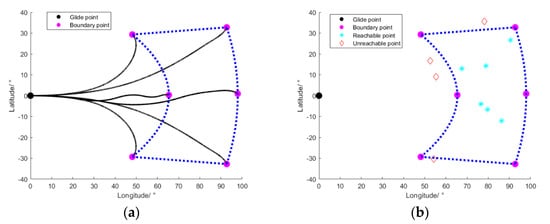
Figure 5.
The reachability discriminant for new target points by SPM: (a) is the travel history; (b) is the reachability discriminant result.
Table 2.
The six boundary points of the reachable zone.
Case 2: Reachability discriminant for new target points. Ten sets of new points were randomly generated in the range of longitude , latitude , and reachability discriminant results, as shown in Table 3; four of the new target points were predicted to be outside the reachable domain and six to be inside, with a success rate of 100% as shown in Figure 5.
Table 3.
Reachability tests for the random points.
5.2. Example 2: DBM Case
In this subsection, five examples are set up to illustrate the advantages of the DBM method in terms of computational accuracy and time efficiency. The simulation configuration parameters set for these cases are shown in Table 1 and Table 4.
Table 4.
Terminal condition configuration for five cases.
Case 0: Reachable zone history. The reachable zone’s history is shown in Figure 6.
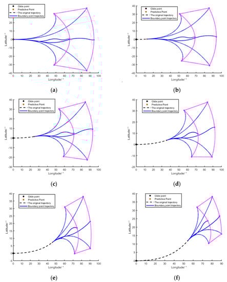
Figure 6.
The history of the reachable zone: (a) is tp = 0 s; (b) is tp = 200 s; (c) is tp = 400 s; (d) is tp = 600 s; (e) is tp = 800 s; (f) is tp = 1000 s.
As shown in Figure 6, the area of the reachable zone of the vehicle decreases as the predicted time of the vehicle progresses. A polynomial curve was fitted to each boundary point versus the predicted time to obtain the trajectories of the changes in position of the six boundary points, as shown in Figure 7, and the positions of the six boundary points of the reachable zone are related to the predicted time.
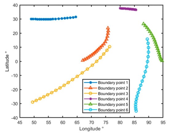
Figure 7.
The position changing of the six boundary points.
What impresses researchers deeply about the proposed method is its accuracy and applicability in the online calculation of the reachable zone. The performance of the DBM in these two aspects will be verified next.
It was already known in advance that the gliding vehicle would fly under the standard condition that it would track the pre-planned D-V profile when . Additionally, assume that an unusual event occurs in the vehicle at the moment ; here, we choose a predicted time randomly to replace this incident. Then, six boundary points would be interpolated at the moment based on the database that has already been created offline, and the close reachable zone would be fitted to the current state of the vehicle online. Furthermore, a new target point would be quickly discriminated against whether it is within the reachable zone or not. As a comparison, the reachable zone determined by the trajectory integration method (TIM) will be employed. In addition, the error of distance is determined by the ratio of the absolute distance value of (DBM–TIM) to the range to go.
The following properties of the DBM are inferred compared with the simulation results mentioned above:
- Adaptability: The reachable zone database can be created offline in advance using the typical trajectories of various initial states and terminal states. As shown in Figure 8, the reachable zone at the present time can be immediately predicted by the DBM when the aircraft is in an emergency. As a result, this method has good adaptability and robustness.
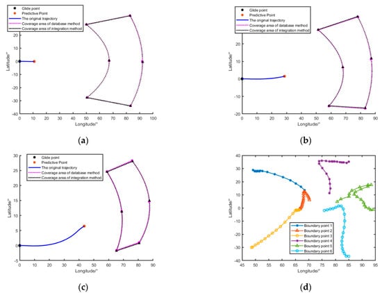 Figure 8. The result of case 1: (a) is tp = 175 s; (b) is tp = 475 s; (c) is tp = 775 s; (d) is the boundary point trajectory.
 - Accuracy: As shown in Table 5, the relative error of the reachable zone’s boundary points obtained by the DBM is within 1%, which provides a guarantee of safe control in the gliding phase of hypersonic vehicles. However, the accuracy decreases with the number of bank reversals and the prediction time.
Table 5. The relative errors of the six boundary points.
- Efficiency: As shown in Table 6, the database method can quickly obtain the reachable zone for the current state of the vehicle in about 0.01s, while the average time for the TIM to calculate the reachable zone is 5–10s. The DBM is therefore more than 90% more efficient in its calculations.
Table 6. Time consumed between TIM and DBM.
6. Conclusions
Aiming at problems such as low computational efficiency and poor adaptability in the target reachable zone prediction of a boosting gliding vehicle, the database method and six-point method are proposed. Firstly, to increase time efficiency, the six-point method, which can determine whether a new goal point is reachable, is first presented. Secondly, the database method for vehicle reachable zone prediction which can provide the potential for online replanning is suggested depending on the six-point method. Finally, the results suggest that the database method achieves very high time efficiency with less loss of accuracy than the six-point method. With an accuracy error of less than 1%, it can forecast the vehicle’s reachable zone within 0.02 s, which is a significant improvement over the integral method, providing a fast guarantee of safe re-entry control for hypersonic vehicles. However, the accuracy declines with an increased number of standard bank reversals, which is a relevant component for additional study in this method.
Author Contributions
Conceptualization, Q.H. and Z.D.; methodology, Q.H.; software, Q.H.; validation, Q.H., Z.D., and L.L.; formal analysis, Q.H.; writing—original draft preparation, Q.H.; writing—review and editing, Z.D. and L.L.; supervision, L.L.; project administration, L.L. All authors have read and agreed to the published version of the manuscript.
Funding
This research was funded by the National Natural Science Foundation of China, grant number 61973326.
Institutional Review Board Statement
Not applicable.
Informed Consent Statement
Not applicable.
Data Availability Statement
All data generated or analyzed during this study are included in this published article.
Conflicts of Interest
The authors declare no conflict of interest.
Nomenclature
| Magnitude | Meaning | Units |
| Velocity relative to the Earth | m/s | |
| The flight path angle | deg | |
| The heading angle | deg | |
| , | The longitude and latitude | deg |
| The radius from the Earth’s center to the vehicle center of mass | m | |
| The mass of the vehicle | kg | |
| The reference area | m2 | |
| The angular velocity of the Earth’s rotation | rad/s | |
| , | The component of the Earth’s gravitational acceleration in the direction of the geocentric radius vector and the angular velocity of the Earth’s rotation | m/s2 |
| , and | The lift coefficient, drag coefficient, and lateral force coefficient | |
| The atmospheric density | kg/m3 | |
| The heating rate | W/cm2 | |
| The dynamic pressure | kPa | |
| The load factor | ||
| The angle of attack | deg | |
| The bank angle | deg |
Appendix A
The following are the theoretical model equations for the D-V profile method:
Once the reference D-V profile is determined, the standard lift-to-drag ratio of the vehicle along that designed profile can be found, denoted as .
The exponential atmosphere model is introduced by:
where is the density of the atmosphere at sea level, is a constant, and . Equation (A1) and the drag acceleration expression are derivative of time t on both sides:
Combining Equations (A2) and (A3) yields:
Furthermore, find the second-order time derivatives of Equation (A4) and the expression :
Combining the two equations and applying the ensuing derivation results in:
Find the first-order and second-order time derivatives on both sides of Equation (7):
Substituting Equation (A9) into Equation (A4) and collecting gives:
Substituting Equations (A9) and (A10) into Equation (A8) and collecting gives:
where the subscript means the value under the standard condition.
In general, the interpolations of aerodynamic data are time-independent, and the terms including and in Equation (A12) can be treated as zero. Thus, the standard lift-to-drag ratio is determined by reduction to be:
The vehicle will also be guided to the predetermined target by a longitudinal trajectory tracking controller, and the required lift-to-drag ratio and its small increment will be determined by:
To maintain the true profile of the vehicle as closely as possible to the reference profile and to provide a smooth transition of the guidance process, the small increment of the required lift-to-drag ratio is designed as follows:
where , , , and are also small increments. It is supposed that the real profile of the vehicle is close to the standard designed profile. The small increments are given by:
Taking the variation of small increments , , , and into Equation (A7), only the first-order terms are retained:
Normally, the angle of attack and bank angle are regarded as the two key control variables in the tracking guidance for a vehicle with the D-V profile method. For the purpose of simplification, the angle of attack can be designed as a segmental linear function of velocity. Therefore, tracking and guiding the vehicle can be accomplished by simply adjusting the bank angle. For further study, if the equations are expanded by perturbation at the current velocity point, some varying components are obtained directly as follows:
Thus, Equation (A17) can be simplified to:
Substituting Equation (A15) into it and collecting with some algebraic skills gives:
It is obvious that Equation (A20) is a second-order ordinary differential equation with an oscillatory form of the solution when . By writing in the standard form:
where and are two designed constants.
Combining Equations (A20) and (A21) and collecting with some algebraic skills, there is:
Because it is difficult to obtain the value of , it can be substituted by , and then the small increment is written as:
Taking the variation of the small increments , , , and into Equation (16), only the first-order terms are retained:
Substituting Equation (A24) into Equation (A15) and collecting with some algebraic skills, there is:
Thus, the required lift-to-drag ratio is given by:
References
- Mutra, R.R.; Mallikarjuna Reddy, D.; Srinivas, J.; Sachin, D.; Babu Rao, K. Signal-based parameter and fault identification in roller bearings using adaptive neuro-fuzzy inference systems. J. Braz. Soc. Mech. Sci. Eng. 2022, 45, 45. [Google Scholar] [CrossRef]
- Hu, K.-Y.; Yang, C.; Sun, W. Adaptive Sliding Mode Fault Compensation for Sensor Faults of Variable Structure Hypersonic Vehicle. Sensors 2022, 22, 1523. [Google Scholar] [CrossRef]
- Zhang, W.; Chen, W.; Yu, W. Analytical solutions to three-dimensional hypersonic gliding trajectory over rotating Earth. Acta Astronaut. 2021, 179, 702–716. [Google Scholar] [CrossRef]
- Yu, W.; Yang, J.; Chen, W.; Liao, B.; Zhu, H. Analytical trajectory prediction for near-first-cosmic-velocity atmospheric gliding using a perturbation method. Acta Astronaut. 2021, 187, 79–88. [Google Scholar] [CrossRef]
- Yu, W.; Chen, W.; Jiang, Z.; Zhou, H.; Liu, X.; Liu, M. Analytical entry guidance based on pseudo-aerodynamic profiles. Aerosp. Sci. Technol. 2017, 66, 315–331. [Google Scholar] [CrossRef]
- Wu, D.; Cheng, L.; Jiang, F.; Li, J. Rapid generation of low-thrust many-revolution earth-center trajectories based on analytical state-based control. Acta Astronaut. 2021, 187, 338–347. [Google Scholar] [CrossRef]
- Yu, W.; Chen, W. Entry guidance with real-time planning of reference based on analytical solutions. Adv. Space Res. 2015, 55, 2325–2345. [Google Scholar] [CrossRef]
- Zhang, W.; Chen, W.; Yu, W.; Zhao, C. Autonomous Entry Guidance based on 3-D Gliding Trajectory Analytical Solution. In Proceedings of the 10th International Conference on Mechanical and Aerospace Engineering (ICMAE), Brussels, Belgium, 22–25 July 2019; pp. 24–31. [Google Scholar]
- Yu, W.; Chen, W.; Jiang, Z.; Zhang, W.; Zhao, P. Analytical entry guidance for coordinated flight with multiple no-fly-zone constraints. Aerosp. Sci. Technol. 2019, 84, 273–290. [Google Scholar] [CrossRef]
- Harpold, J.C.; Graves, C.A. Shuttle program. Shuttle entry guidance. J. Astronaut. Sci. 1979, 27, 239–268. [Google Scholar]
- Harpold, J.C.; Gavert, D.E. Space Shuttle entry guidance performance results. J. Guid. Control. Dyn. 1983, 6, 442–447. [Google Scholar] [CrossRef]
- Zhang, Y.-L.; Chen, K.-J.; Liu, L.-H.; Tang, G.-J.; Bao, W.-M. Entry trajectory generation based on quasi-three-dimensional acceleration guidance. In Proceedings of the 35th Chinese Control Conference (CCC), Chengdu, China, 27–29 July 2016; pp. 5313–5319. [Google Scholar] [CrossRef]
- Zhang, Y.-L.; Xie, Y.; Peng, S.-C.; Tang, G.-J.; Bao, W.-M. Entry trajectory generation with complex constraints based on three-dimensional acceleration profile. Aerosp. Sci. Technol. 2019, 91, 231–240. [Google Scholar] [CrossRef]
- Xie, Y.; Liu, L.; Tang, G.; Zheng, W. Highly constrained entry trajectory generation. Acta Astronaut. 2013, 88, 44–60. [Google Scholar] [CrossRef]
- Wang, J.; Wu, Y.; Liu, M.; Yang, M.; Liang, H. A Real-Time Trajectory Optimization Method for Hypersonic Vehicles Based on a Deep Neural Network. Aerospace 2022, 9, 188. [Google Scholar] [CrossRef]
- Benito, J.; Mease, K.D. Reachable and Controllable Sets for Planetary Entry and Landing. J. Guid. Control. Dyn. 2010, 33, 641–654. [Google Scholar] [CrossRef]
- Hsu, F.-K.; Kuo, T.-S.; Chern, J.-S. Landing domain analysis of shuttle re-entry vehicles. Int. J. Syst. Sci. 1991, 22, 1145–1158. [Google Scholar] [CrossRef]
- Chen, S.Y. The Longitudinal and Lateral Range of Hypersonic Glide Vehicles with Constant Bank Angle; RAND Corporation: Santa Monica, CA, USA, 1966. [Google Scholar]
- Nyland, F.S. Hypersonic Turning with Constant Bank Angle Control. Space Technology and Science; RAND Corporation: Santa Monica, CA, USA, 1965. [Google Scholar]
- Arslantas, Y.E.; Oehschlgel, T.; Sagliano, M.; Theil, S.; Braxmaier, C. In Safe Landing Area Determination for a Moon Lander by Reachability Analysis. In Proceedings of the 65th International Astronautical Conference (IAC), Toronto, ON, Canada, 29 September–3 October 2014. [Google Scholar]
- Gao, C.; Jiang, C.; Jing, W. Optimization of projectile state and trajectory of reentry body considering attainment of carrying aircraft. J. Syst. Eng. Electron. 2017, 28, 137–144. [Google Scholar] [CrossRef]
- Zhao, Z.D.; Cui, P.Y.; Zhu, S.Y. An Analytical Homotopic Method to Generate the Reachable Longitudinal Area for Mars Entry. J. Astronaut. 2019, 40, 1024–1033. [Google Scholar]
- Xu, J.; Dong, C.; Cheng, L. Deep Neural Network-Based Footprint Prediction and Attack Intention Inference of Hypersonic Glide Vehicles. Mathematics 2022, 11, 185. [Google Scholar] [CrossRef]
- Zeng, X.; Zhong, F.; Ding, X.; Huifeng, L.I.; Cheng, X. Method for Landing Footprint Generation in Reusable Vehicles. Manned Spacefl. 2017, 23, 14–20. [Google Scholar]
- He, R.-Z.; Zhang, Y.-L.; Liu, L.-L.; Tang, G.-J.; Bao, W.-M. Feasible footprint generation with uncertainty effects. Proc. Inst. Mech. Eng. Part G J. Aerosp. Eng. 2017, 233, 138–150. [Google Scholar] [CrossRef]
- Mease, K.D.; Kremer, J.-P. Shuttle entry guidance revisited using nonlinear geometric methods. J. Guid. Control. Dyn. 1994, 17, 1350–1356. [Google Scholar] [CrossRef]
- Saraf, A.; Leavitt, J.A.; Chen, D.T.; Mease, K.D. Design and Evaluation of an Acceleration Guidance Algorithm for Entry. J. Spacecr. Rocket. 2003, 41, 986–996. [Google Scholar] [CrossRef]
Disclaimer/Publisher’s Note: The statements, opinions and data contained in all publications are solely those of the individual author(s) and contributor(s) and not of MDPI and/or the editor(s). MDPI and/or the editor(s) disclaim responsibility for any injury to people or property resulting from any ideas, methods, instructions or products referred to in the content. |
© 2023 by the authors. Licensee MDPI, Basel, Switzerland. This article is an open access article distributed under the terms and conditions of the Creative Commons Attribution (CC BY) license (https://creativecommons.org/licenses/by/4.0/).