Interacting Multiple Model Filter with a Maximum Correntropy Criterion for GPS Navigation Processing

Abstract

In order to deal with the uncertainty of measurement noise, particularly for outlier types of multipath interference and non-line of sight (NLOS) reception, this paper proposes a novel method for processing the navigation states of the Global Positioning System (GPS) that combines the maximum correntropy criterion (MCC) and the interacting multiple model (IMM), with an extended Kalman Filter (EKF). Multipath mitigation is essential for increased positioning accuracy since multipath interference is one of the primary sources of errors. Nonlinear filtering with IMM configuration uses filter structural adaptation. In processing time-varying satellite signal standards for GPS navigation, it offers an alternative for creating the adaptive filter. A collection of switching models built on a method of multiple model estimation can be used to characterize the uncertainty of the noise. Even though most noise in real life is non-Gaussian, time-varying, and of fluctuating strength, the standard EKF operates effectively when the noise is Gaussian. The performance of EKF will drastically decline if the signals appear non-Gaussian. The underlying system disrupted by heavy-tailed, non-Gaussian impulsive sounds could be better since the EKF employs second-order statistical information. The MCC is a method for comparing two random variables based on higher-order signal statistics. The maximum correntropy-extended Kalman filter (MCEKF), which uses the MCC rather than the minimal mean square error (MMSE) as the optimization criterion, is used to enhance performance in non-Gaussian situations. Finally, a performance evaluation will be conducted to compare the effectiveness of the suggested strategy in improving positioning to alternative system designs.

1. Introduction

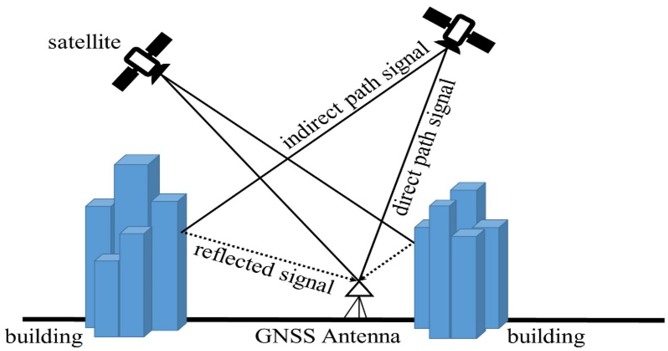
Global Navigation Satellite Systems (GNSS), such as the Global Positioning System (GPS), have severe inaccuracies in urban environments due to multipath interference and non-line of sight (NLOS) reception [1,2]. Multipath interferences are common in urban, forested, and terrain with significant valleys or mountains. For instance, a narrow downtown street with tall buildings on either side has poor GPS reception. Furthermore, when a signal’s direct line of sight (LOS) is obstructed, it can only be received via reflection, known as NLOS reception. In extreme multipath conditions, the LOS signal may be blocked entirely, leaving only the reflected signals. The code correlation peak is distorted by the reflected signals, making it difficult to detect the precise code phase of the direct LOS signal. Multipath errors as shown in Figure 1 are spatially uncorrelated errors that cannot be eliminated by observational differential processing, in contrast to some other correlated types of errors, such as the ionospheric and tropospheric errors.

Observations that deviate significantly from most of the observation sample are known as outliers. One of the primary sources of inaccuracy for high-accuracy positioning systems is the irrelevancy between different instants and the appearance of uncertainty during the observation period. Despite the precautions taken throughout the observation period and the enhanced models used to eliminate systematic errors, observations may still be tainted by outliers, which frequently lower the quality of the estimated states and make them unreliable for any significant interference. Smoothing the ranging results can increase accuracy by reducing NLOS propagation’s effects.

A well-known estimator based on minimal mean square error (MMSE) is the Kalman filter (KF) [3]. It is generally accepted that, in linear systems with white Gaussian noise, KF uses MMSE as the best criterion. However, non-Gaussian sounds are frequently present in many real-world settings and can cause a significant decline in performance. Furthermore, the extended Kalman filter (EKF), an extension of the linear Kalman filter for handling nonlinear systems, will degrade if non-Gaussian noise disturbs the system. The process and measurement noises’ high-order information is not utilized by the EKF when the noise exhibits non-Gaussianity. Numerous severe flaws in the EKF and unscented Kalman filter (UKF) techniques prevent widespread use. The non-Gaussian process and observation noises of the models and the unknowable noise covariance matrices are unique issues they cannot be managed. Additionally, because the estimated results are susceptible to significant outliers and non-Gaussian noise, the EKF struggles when the systems are combined with colored noise, which occurs in many real-world application settings. Despite being capable of handling non-Gaussian, nonlinear systems, the particle filter (PF) requires a significant investment in computing power for online implementation.

The extent to which the EKF’s performance depends on a predefined dynamic model is one major inconvenience. The designers must know the dynamic process and measurement models beforehand and assume that a zero-mean Gaussian white noise corrupts both models to provide accurate estimation results. The state vector has been estimated using the innovation-based adaptive Kalman filter (AKF) [4,5] technique to avoid divergence brought on by incorrect modeling. Additionally, a process that is adaptable can be used to identify modeling flaws or system model uncertainty dynamically. The model-matched state estimation filters that are running concurrently in the interacting multiple model (IMM) algorithm [6,7,8,9,10,11,12] exchange information (interact) at each sampling period. Target-tracking applications were the first to use the IMM method, followed by navigation applications. A model probability evaluator first determines the likelihood that the receiver dynamic is currently in each potential mode. The most recent mode probabilities are then used to construct a global estimate of the user’s condition. The method implements a gentle switch between the various modes by modifying the probabilities of each mode, which are used as weightings in the aggregate global state estimate. This combined estimate’s covariance matrix considers the similarities and differences between the mode-conditioned estimates. Two models were constructed for this study’s many models, each describing a different aspect of observation. The IMM algorithm weighs the inputs and outputs of a bank of parallel filters at each instant using model probabilities.

The idea of entropy has recently found widespread use in information theoretic learning (ITL), where the minimum error entropy (MEE) and maximum correntropy criteria (MCC) [13,14,15,16,17,18,19,20] are most often employed for robust filter design dealing with non-Gaussian system applications. By integrating the probability density function (pdf), the statistical measure correntropy calculates the similarity between two or more variables. To mitigate non-Gaussian noise, the accompanying MCC is used as a new cost function for robust filtering. The MCC was created using an ITL methodology and has been applied effectively in various filter design applications, mainly when non-Gaussian sounds are present. Furthermore, to address the estimation problems in non-Gaussian noise settings, the MCC was used to replace the MSE criteria in developing a robust EKF known as the MCEKF. Some other well-known robust filter designs are available based on the relative entropy (also called the Kullback–Leibler divergence) or minimax theory [21,22].

The MCEKF frequently performs far better than the conventional EKF. It has been stated that MCC is better suited for unknown noise and undetermined parameters and has a close link with M-estimators. A new general answer for researching random systems with generalized noise is also shown. MCEKF uses the MCC rather than the MMSE as the optimization criterion for GNSS navigation processing to improve the performance of EKF applications where non-Gaussian disturbances are present. The ranging error space may be constrained using the measured distance and its variance, controlled to exclude the impacts of colored Gaussian noise. By integrating the MCEKF and IMM technologies, the proposed IMM–MCEKF offers higher non-Gaussian signal processing performance. Furthermore, the IMM–MCEKF was demonstrated to be more effective in processing non-Gaussian data by combining IMM and MCC-based EKF algorithms. As a result, the MCC is used in this work in place of the conventional MMSE criteria for GPS navigation.

The rest of this paper is structured as follows. The interacting multiple-model based filter is introduced in Section 2. The maximum correntropy-extended Kalman filter is shown in Section 3. The proposed IMM–MCEKF’s performance compared to the EKF, IMM-EKF, and MCEKF techniques is assessed using illustrative examples based on simulation experiments in Section 4. Finally, Section 5 provides conclusions.

2. The Interacting Multiple Model Filters

Consider a single model equation in the discrete-time form:

$$x_k=f_{k-1}(x_{k-1})+w_{k-1}$$

(1)

$$z_k=h_k(x_k)+v_k$$

(2)

where the state vector $x_k\in {\Re }^n$, the process noise vector $w_k\in {\Re }^m$, the measurement vector $z_k\in {\Re }^m$, and the measurement noise vector $v_k\in {\Re }^m$, $Q_k$ is the process noise covariance matrix, and $R_k$ is the measurement noise covariance matrix.

2.1. Extended Kalman Filter

The vectors $w_k$ and $v_k$ in Equations (1) and (2) are zero-mean Gaussian white sequences with zero cross-correlation with each other:

$$E[w_k{w}_i^{\mathrm{T}}]=Q_k{\delta }_{ik}; E[v_k{v}_i^{\mathrm{T}}]=R_k{\delta }_{ik}; E[w_k{v}_i^{\mathrm{T}}]=0\hspace{1em}\hspace{1em}for\hspace{0.33em}all\hspace{0.33em}i\hspace{0.33em}and\hspace{0.33em}k$$

where $E\hspace{0.17em}[·]$ represents mathematical expectation and the superscript “T” denotes the matrix transpose. The symbol ${\delta }_{ik}$ stands for the Kronecker delta function given by:

$${\delta }_{ik}=\left\{\begin{array}{c}1,\begin{array}{cc}& i=k\end{array}\\ 0,\begin{array}{cc}& i\ne k\end{array}\end{array}\right.$$

The discrete-time EKF algorithm is summarized as follows:

(1)

Initialize state vector ${\widehat{x}}_{0|0}$ and state covariance matrix $P_{0|0}$.

(2)

Predict the state vector and state covariance matrix:

$${\widehat{x}}_{k|k-1}=f_{k-1}({\widehat{x}}_{k-1|k-1})$$

$$P_{k|k-1}={\Phi }_{k-1}{P}_{k-1|k-1}{\Phi }_{k-1}^T+Q_{k-1}$$

(3)

Compute the Kalman gain matrix: $K_k=P_{k|k-1}{H}_k^{\mathrm{T}}{[H_k{P}_{k|k-1}{H}_k^{\mathrm{T}}+R_k]}^{-1}$.

(4)

Update the state vector: ${\widehat{x}}_{k|k}={\widehat{x}}_{k|k-1}+K_k[z_k-h_k({\widehat{x}}_{k|k-1})]$.

(5)

Update the error covariance: $P_{k|k}=\left[I-K_k{H}_k\right]P_{k|k-1}$.

where the linear approximation equations for the system and measurement matrices are obtained through the following relations:

$${\Phi }_{k-1}\approx {\left.\frac{\partial f_k}{\partial x}\right|}_{x={\widehat{x}}_{k|k-1}}; H_k\approx {\left.\frac{\partial h_k}{\partial x}\right|}_{x={\widehat{x}}_{k|k-1}}$$

2.2. The Framework of the Interacting Multiple Model Filter

The IMM algorithm utilizes two or more models to describe the possible states. Let a general system for multiple models in discrete time be defined by

$$x_k=f_{k-1}(x_{k-1},M_{k-1})+w_{k-1}(M_{k-1})$$

(3)

$$z_k=h_k(x_k,M_k)+v_k(M_k)$$

(4)

where $f_k(·)$ and $h_k(·)$ are the parameterized state transition and measurement functions, respectively; $x_k$ and $z_k$ are the dynamical state and measurement of the system, respectively, in the model $M_k$, where the system itself is a Markov chain; $w_k$ and $v_k$ are the process noise and measurement noise, with the means $w_k$ and $v_k$ and covariances $Q_k$ and $R_k$, respectively. The effective weighted fusion estimates the system state vector and allows the real-time correction of the state variables such as location and velocity. This flexibility can solve the problem of substantial single-model estimating inaccuracy. Furthermore, the algorithm of IMM-involved nonlinear filters was introduced to address both system nonlinearity and noise uncertainty at once.

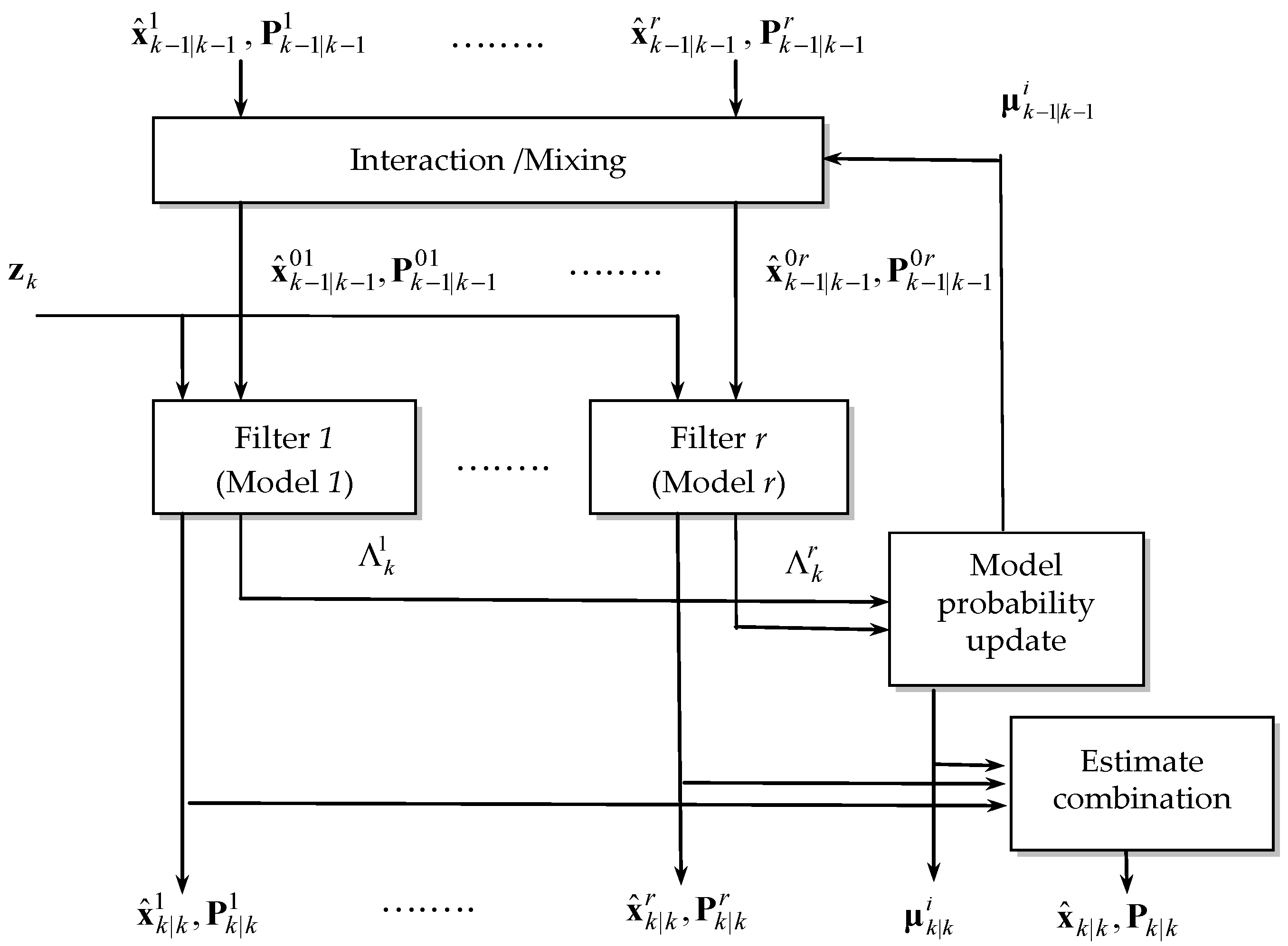
The IMM approach integrates state possibilities from several filter models for time-varying models to obtain an improved state estimate. One can select the IMM filter model for each state hypothesis that best fits the behavior of the target systems. The primary strength of the IMM algorithm is its capacity to predict the state of a dynamic system with many behavior modes that can “switch” between them. The IMM technique uses the model probability to implement a “soft switch” between different models. The construction of the IMM-based estimator for the scenario involving the involved r models is shown in Figure 2. The IMM algorithm weighs the input and output of parallel filters at each instant using model probabilities. The strategy considers several models to reflect the system’s model or behavior patterns. Combining the different estimates from the filters running in parallel based on the many models that match the system modes yields the overall estimate. There are four phases in each IMM cycle: (1) interaction, (2) filtering, (3) calculation of the mode probability, and (4) combination. The four key stages of the IMM–EKF algorithm are divided as shown in the following list:

(1)

Model interaction/mixing

For the given states $x_{k-1}^j=x_{k-1|k-1}^j$ with the corresponding covariances $P_{k-1}^j=P_{k-1|k-1}^j$ and mixing probabilities ${{\displaystyle \mathsf{\mu }}}_{k-1|k-1}^{i|j}$ for every model, the initial condition for the model $j$ is

$${{\displaystyle \widehat{x}}}_{k-1|k-1}^{0j}={\displaystyle \sum _{i=1}^r{{\displaystyle \widehat{x}}}_{k-1|k-1}^i}{{\displaystyle {\displaystyle \mathsf{\mu }}}}_{k-1|k-1}^{i|j}, j=1,2,\dots ,r$$

(5)

The covariance corresponding to the above is:

$$P_{k-1|k-1}^{0j}={\displaystyle \sum _{i=1}^r{{\displaystyle \mathsf{\mu }}}_{k-1|k-1}^{i|j}\{P_{k-1|k-1}^i}+[{\widehat{x}}_{k-1|k-1}^i-{\widehat{x}}_{k-1|k-1}^{0j}]{[{\widehat{x}}_{k-1|k-1}^i-{\widehat{x}}_{k-1|k-1}^{0j}]}^{\mathrm{T}}\}$$

(6)

The model transition probabilities are related to the Markov chain and are defined as:

$$\mathrm{\Pi }=p{\displaystyle \left\{M_k^j\right|M_{k-1}^i\}}=\left[\begin{array}{cccc}{\pi }_{11}& {\pi }_{12}& \dots & {\pi }_{1j}\\ {\pi }_{21}& {\pi }_{22}& \dots & {\pi }_{2j}\\ ⋮& ⋮& \ddots & ⋮\\ {\pi }_{i1}& {\pi }_{i2}& \dots & {\pi }_{ij}\end{array}\right]$$

(7)

where $i,j=1,2,\dots , r$, and $r$ is the number of sub-models. The calculations of the mixing probabilities with mode switching probability matrix ${{\displaystyle \pi }}_{ij}$ and the Gaussian mixing probabilities are expressed by:

$${{\displaystyle {\displaystyle \mathsf{\mu }}}}_{k-1|k-1}^{i|j}=\frac{1}{{\overline{c}}_j}{{\displaystyle \pi }}_{ij}{{\displaystyle {\displaystyle \mathsf{\mu }}}}_{k-1}^i, i,j=1,\dots ,r$$

(8)

where ${{\displaystyle \overline{c}}}_j$ is a normalization factor given by

$${{\displaystyle \overline{c}}}_j={\displaystyle \sum _{i=1}^r{{\displaystyle \pi }}_{ij}{{\displaystyle {\displaystyle \mathsf{\mu }}}}_{k-1}^i}$$

where ${{\displaystyle \widehat{x}}}_{k-1|k-1}^{0j}$ and ${\widehat{P}}_{k-1|k-1}^{0j}$ are the mixed initial conditions for mode-matched filter $j$ at time $k-1$. Notice that $i$ and $j$ denote the corresponding model index and n is the total number of sampling particles.

(2)

Filtering

The state estimate equation and covariance equation are inputs to the filter matched to $M_k^j$, which employs $z_k$ to yield ${\widehat{x}}_{k|k}^j$ and $P_{k|k}^j$. The likelihood function corresponding to the $r$ filters

$${{\displaystyle \mathrm{\Lambda }}}_k^j=p[{{\displaystyle z}}_k|M_k^j,{{\displaystyle Z}}_{k-1}]$$

(9)

which are computed through the mixed initial condition given by

$${{\displaystyle \mathrm{\Lambda }}}_k^j=p[z_k|M_k^j,{{\displaystyle \widehat{x}}}_{k-1|k-1}^{0j},{{\displaystyle P}}_{k-1|k-1}^{0j}]$$

(10)

(3)

Model probability update

The model probability ${{\displaystyle \mathsf{\mu }}}_k^j$ is updated according to the model likelihood and model transition probability governed by the finite-state Markov chain:

$${{\displaystyle \mathsf{\mu }}}_k^j=\frac{1}{c}\mathrm{\Lambda }\overline{c}kj{}_j$$

(11)

where

$$c={\displaystyle \sum _{j=1}^r{\overline{c}}_j\mathrm{\Lambda }kj}$$

(12)

and $\mathrm{\Lambda }kj$ is a likelihood function given by

$${\mathrm{\Lambda }}_k^j=\frac{1}{\sqrt{2\pi \left|P_{zz}^j\right|}}\exp \left[-\frac{1}{2}{\upsilon }_k^j{}^{\mathrm{T}}{(P_{zz}^j)}^{-1}{\upsilon }_k^j\right]$$

(13)

(4)

Combination of state estimation

The model-conditioned estimates and covariances, respectively, are combined according to the mixture equations

$${\widehat{x}}_{k|k}={\displaystyle \sum _{j=1}^r{{\displaystyle \mathsf{\mu }}}_k^j{\widehat{x}}_{k|k}^j}$$

(14)

$$P_{k|k}={\displaystyle \sum _{j=1}^r{{\displaystyle \mathsf{\mu }}}_k^j\{P_k^j+[{\widehat{x}}_{k|k}^j-{\widehat{x}}_{k|k}]{[{\widehat{x}}_{k|k}^j-{\widehat{x}}_{k|k}]}^{\mathrm{T}}\}}$$

(15)

3. Extended Kalman Filter with Maximum Correntropy

A strategy for non-parametrically adapting systems based on entropy and divergence is information theoretic learning. In information theory, entropy measures the uncertainty associated with random variables. Since Shannon initially proposed entropy in 1948 [23], several definitions, including those by Renyi and Shannon, have been developed for various purposes. For example, correntropy has been widely employed in machine learning and adaptive filtering to ascertain the local similarity of random variables. The MCC-based algorithms are further resistant to non-Gaussian noise, mainly when impulse noise is present.

Information theoretic and kernel approaches define the correntropy between two random variables provided in a kernel space as a generalized local similarity measure. MCC has approved many applications. For instance, MCC has benefited from signal processing, pattern recognition, and machine learning. This section introduces MCC and extended Kalman filters to deal with non-white Gaussian noise, notably the outliers.

The correntropy of two scalar random variables measures the second and higher orders of statistical data in the joint probability density function. The metric similarity between two variables is measured by correntropy. The correntropy of two scalar random variables, X and Y, is defined as

$$V_{\sigma }(X,Y)=E[k_{\sigma }(X,Y)]={\displaystyle \iint k_{\sigma }(x,y)f_{XY}(x,y)dxdy}$$

(16)

where $k_{\sigma }(x,y)=G_{\sigma }(e)$ is a positive definite kernel function that satisfies the Mercer theory, $f_{XY}(x,y)$ is the joint probability density function, and $E[·]$ represents the expectation operator. The provided Gaussian kernel is one of the kernel functions that are most frequently utilized.

$$k_{\sigma }(x,y)=G_{\sigma }(e)=\frac{1}{\sqrt{2\pi }\sigma }\exp \left(-\frac{e^2}{2{\sigma }^2}\right)$$

(17)

When the kernel bandwidth is determined by $e=x-y$, $\sigma >0$, the joint distribution F(X, Y) is usually inaccessible. This is so because we might only have access to a certain amount of data in most real-world circumstances. The correntropy can be calculated using a sample mean square of the data to deal with this problem. Since there is often a dearth of data and a limited amount of information, the joint distribution is typically unknown in most real-world settings. When determining the correntropy from N samples, the sample mean estimator can be employed in the following circumstances:

$${\widehat{V}}_{\sigma }(X,Y)=\frac{1}{N}{\displaystyle \sum _{i=1}^N{k}_{\sigma }(x_i,y_i)}$$

(18)

which, in terms of Gaussian kernel, can be written as

$${\widehat{V}}_{\sigma }(X,Y)=\frac{1}{N}{\displaystyle \sum _{i=1}^N{G}_{\sigma }(x_i-y_i)}=\frac{1}{N}{\displaystyle \sum _{i=1}^N{G}_{\sigma }(e_i)}$$

(19)

Taking the Taylor series expansion of the Gaussian kernel, we have

$$V_{\sigma }(X,Y)=\frac{1}{\sqrt{2\pi \sigma }}{\displaystyle \sum _{n=0}^{\infty }\frac{{(-1)}^n}{2^n{\sigma }^{2n}n!}E\left[{(X-Y)}^{2n}\right]}$$

(20)

The weighted average of all the even-order error variable moments is correntropy, as seen in (X – Y). The kernel bandwidth is a factor that determines how heavily the second and higher-order moments are weighted. The second-order moment will predominate in the correntropy in the presence of a large kernel bandwidth $\sigma$ (in comparison to the dynamic range of the data).

The MCC serves as the basis for deriving the nonlinear version of the linear Kalman filter in detail from the linear version in [15]. An alternative objective function might be created, and its robustness increased using the weighted least squares (WLS) approach. Therefore, the objective is to increase the objective function $J_m$ provided by

$$J_m=G_{\sigma }\left(\right||z_k-h({\widehat{x}}_{k|k-1})|{|}_{R_k^{-1}})+G_{\sigma }(\left|\right|{\widehat{x}}_{k|k}-f({\widehat{x}}_{k-1|k-1})\left|{|}_{P_{k|k-1}^{-1}}\right)$$

(21)

Taking the derivative of the objective function $J_m$ with respect to ${\widehat{x}}_{k|k}$ and setting its value to zero

$$\frac{\partial J_m}{\partial {\widehat{x}}_{k|k}}=0$$

(22)

and therefore the following equation can be obtained

$${\widehat{x}}_{k|k}=f({\widehat{x}}_{k-1|k-1})+\frac{G_{\sigma }(||z_k-h({\widehat{x}}_{k|k-1})|{|}_{R_k^{-1}})}{G_{\sigma }(||{\widehat{x}}_{k|k}-f({\widehat{x}}_{k-1|k-1})|{|}_{P_{k|k-1}^{-1}})}{H}_k^{\mathrm{T}}(z_k-h({\widehat{x}}_{k|k-1}))$$

(23)

From Equation (22), we have

$$-\frac{1}{{\sigma }^2}{G}_{\sigma }(||z_k-h({\widehat{x}}_{k|k-1})|{|}_{R_k^{-1}})H_k^T{R}_k^{-1}(z_k-h({\widehat{x}}_{k|k-1}))+\frac{1}{{\sigma }^2}{G}_{\sigma }(\left|\right|{\widehat{x}}_{k|k}-f({\widehat{x}}_{k-1|k-1})|{|}_{P_{k|k-1}^{-1}})P_{k|k-1}^{-1}({\widehat{x}}_{k|k}-f({\widehat{x}}_{k-1|k-1}))=0$$

(24)

which can be written as

$$P_{k|k-1}^{-1}{\widehat{x}}_{k|k}-P_{k|k-1}^{-1}f({\widehat{x}}_{k-1|k-1})=L_k{H}_k^T{R}_k^{-1}(z_k-h({\widehat{x}}_{k|k-1}))$$

(25)

where

$$L_k=\frac{G_{\sigma }(||z_k-h({\widehat{x}}_{k|k-1})|{|}_{R_k^{-1}})}{G_{\sigma }(||{\widehat{x}}_{k|k}-f({\widehat{x}}_{k-1|k-1})|{|}_{P_{k|k-1}^{-1}})}$$

(26)

Since $G_{\sigma }\left(\right||{\widehat{x}}_{k|k}-f({\widehat{x}}_{k-1|k-1})|{|}_{P_{k|k-1}^{-1}})\approx G_{\sigma }(\left|\right|{\widehat{x}}_{k|k-1}-f({\widehat{x}}_{k-1|k-1})\left|{|}_{P_{k|k-1}^{-1}}\right)=1$, we have

$$L_k=G_{\sigma }\left(\right||z_k-h({\widehat{x}}_{k|k-1}){\left|\right|}_{R_k^{-1}})$$

(27)

The resulting estimator is referred to as the maximum correntropy criterion-based EKF, which has the new gain given by

$$K_k={(P_{k|k-1}^{-1}+L_k{H}_k^T{R}_k^{-1}{H}_k)}^{-1}{L}_k{H}_k^T{R}_k^{-1}$$

(28)

which can also be written as

$$K_k=L_k{P}_{k|k-1}{H}_k^{\mathrm{T}}{[L_k{H}_k{P}_{k|k-1}{H}_k^{\mathrm{T}}+R_k]}^{-1}$$

(29)

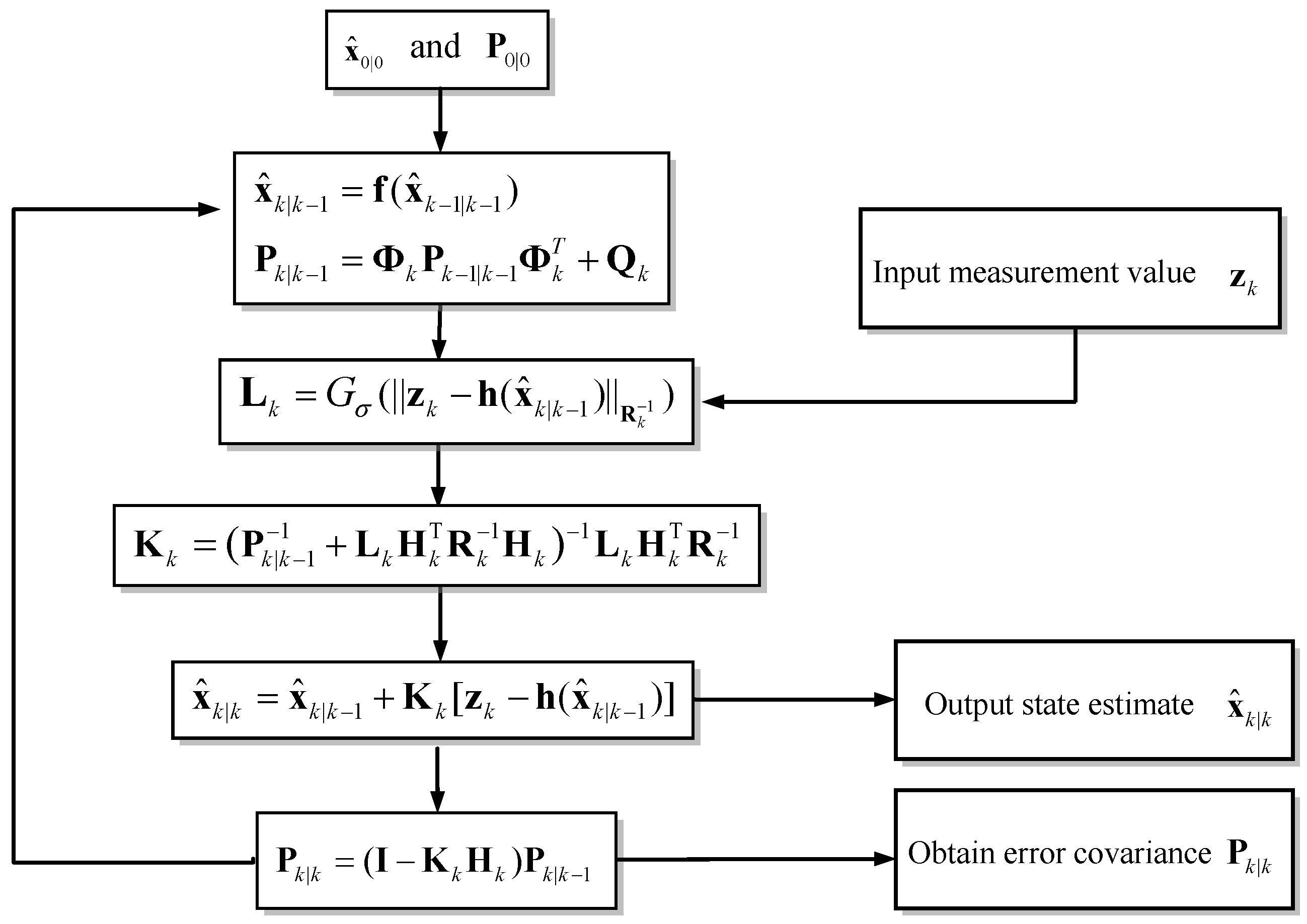
Figure 3 provides the flow chart for the MCC-based EKF. The computation procedures are summarized as follows:

(1)

Initialize state vector and state covariance matrix: ${\widehat{x}}_{0|0}^{}$ and $P_{0|0}^{}$.

(2)

Predict the state vector ${\widehat{x}}_{k|k-1}$ and the state covariance matrix $P_{k|k-1}^{}$.

(3)

Compute the measurement innovation based on maximum correntropy criterion to derive the factor $L_k$.

(4)

Compute the modified Kalman gain matrix $K_k$.

(5)

Update the state vector ${\widehat{x}}_{k|k}$ and the error covariance $P_{k|k}$.

(6)

Repeat from Step (2) to perform the next estimation cycle.

4. Results and Discussion

Simulation experiments were conducted to evaluate the performance of the proposed approach compared to the conventional methods of GPS navigation processing to validate the effectiveness of the proposed approach in the presence of a time-varying satellite signal quality. The various types of navigation filters, including the EKF, IMM–EKF, MCEKF, and IMM–MCEKF, were developed by the authors using the MATLAB^® codes with the Inertial Navigation System (INS) Toolbox [24] and the Satellite Navigation (SatNav) Toolbox [25] commercial software programs, both produced by GPSoft LLC. The vehicle’s trajectory was produced using the INS Toolbox, while the satellite orbits and pseudoranges were created using the SatNav Toolbox.

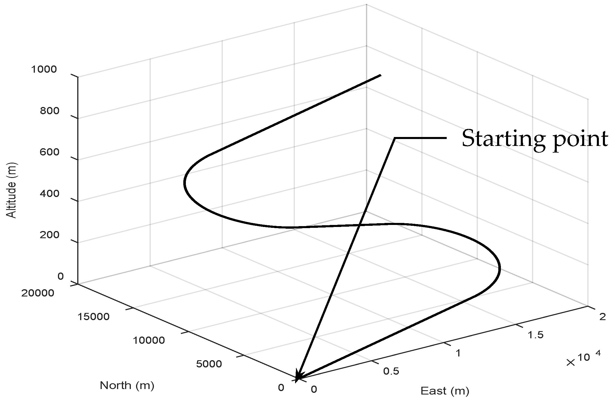
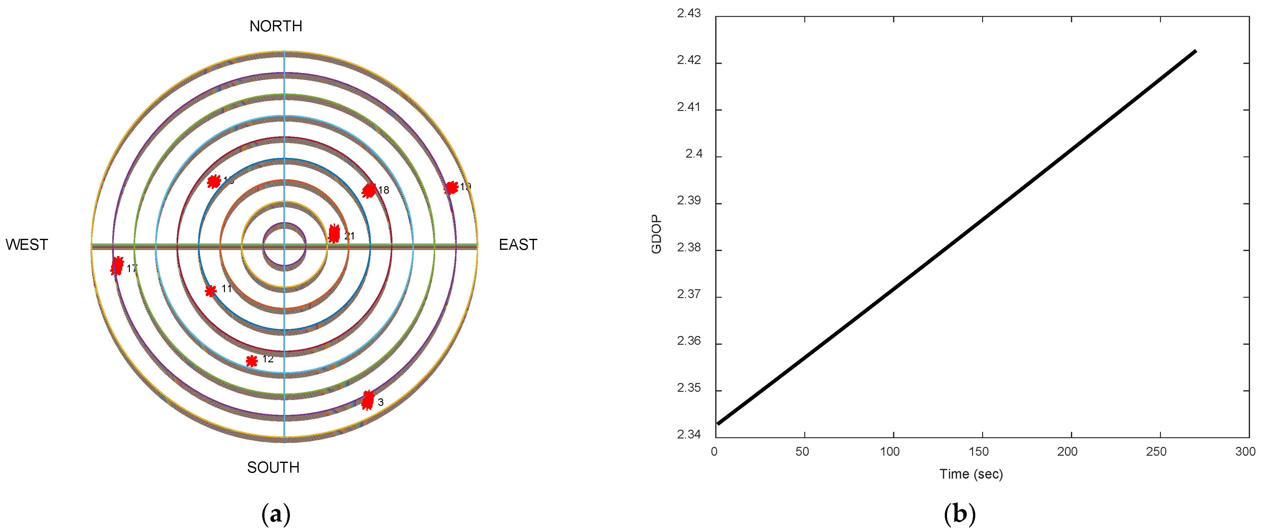
The test trajectory from the simulation is shown in Figure 4. As shown in Figure 5, eight GPS satellites (red colored dots followed by the GPS ID number) are reachable and the corresponding Geometry Dilution of Precision (GDOP) is around 2.4, which is good to assure appropriate navigation satellite geometry on positional measurement precision. Thus, we focused on the investigation of the position errors induced by the pseudorange observables, which reflect the quality of the measurement model in the filters. The simulated vehicle is located at an altitude of 100 m, which is comparable to ${\left[\begin{array}{ccc}-3042329.2& 4911080.2& 2694074.3\end{array}\right]}^{\mathrm{T}}$ m in the WGS-84 ECEF coordinate system. It starts at East 121.7775 degrees and North 25.1492 degrees. The origin is defined as the (0, 0, 0) m point in the local tangent East–North–Up (ENU) frame.

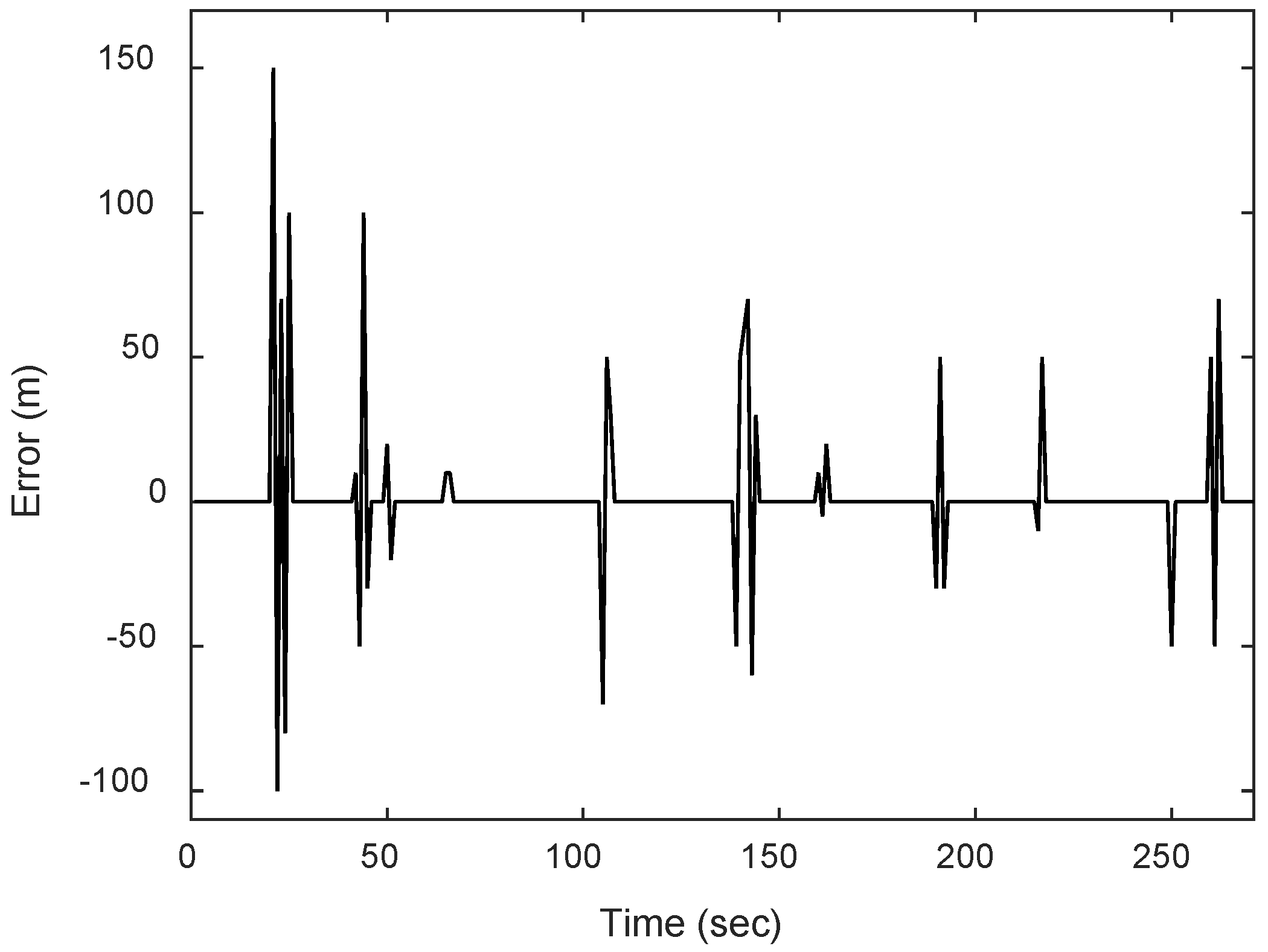
Multiple extras and randomly generated errors were purposefully added to the GPS pseudorange observation data while the vehicle was in motion to assess performance involving outlier type of multipath interferences. The error factors that distort the GPS observables were receiver noise, multipath, ionospheric delay, and tropospheric delay. Further, by assuming that the differential GPS (DGPS) mode was used, most errors were corrected; however, the multipath effect and receiver thermal noise could not be eliminated in this proposed study. The error induced by the receiver thermal noise was considered to be a Gaussian sequence with zero mean and unity variance. In addition, the efficacy of the outlier kind of multipath interference was further evaluated using several other intentionally produced and randomly generated problems. For example, urban areas or environments with NLOS and multipath receptions make it difficult for vehicles to navigate using GNSS data. Furthermore, the introduction of inaccurate data by these occurrences interferes with the precise positioning of the GPS sensor. Figure 6 depicts the sequences of outlier interferences added to the pseudorange observables during the experiment. These measurement errors might be between a few tens and several hundred meters during the coding step.

The IMM approach described in this work handles measurement uncertainty by modifying the $R_k$. Since this study avoided outlier types of multipath interference or NLOS reception, the influence of measurement noise $R_k$ was essential. Therefore, in environments with high levels of multipath, a more significant value of measurement noise covariance $R_k$ should be used; in environments with low levels of multipath, a less significant value of measurement noise covariance $R_k$ should be used. This modeling approach allows various model estimates to address the challenge of nonlinear filtering, given the noise level and distribution uncertainty. A collection of switching models describes the uncertainty of the noise strength. In this work, the idea of several models interacting was intended to reduce measurement uncertainty by modifying $R_k$. The following Markov chain transition probability matrix was used:

$$\mathrm{\Pi }=\left[\begin{array}{cc}{\pi }_{11}& {\pi }_{12}\\ {\pi }_{21}& {\pi }_{22}\end{array}\right]=\left[\begin{array}{cc}0.7& 0.3\\ 0.3& 0.7\end{array}\right]$$

A vehicle is supposed to move continuously to lessen the effects of the $Q_k$ brought on by the unmodeling faults in the system dynamics.

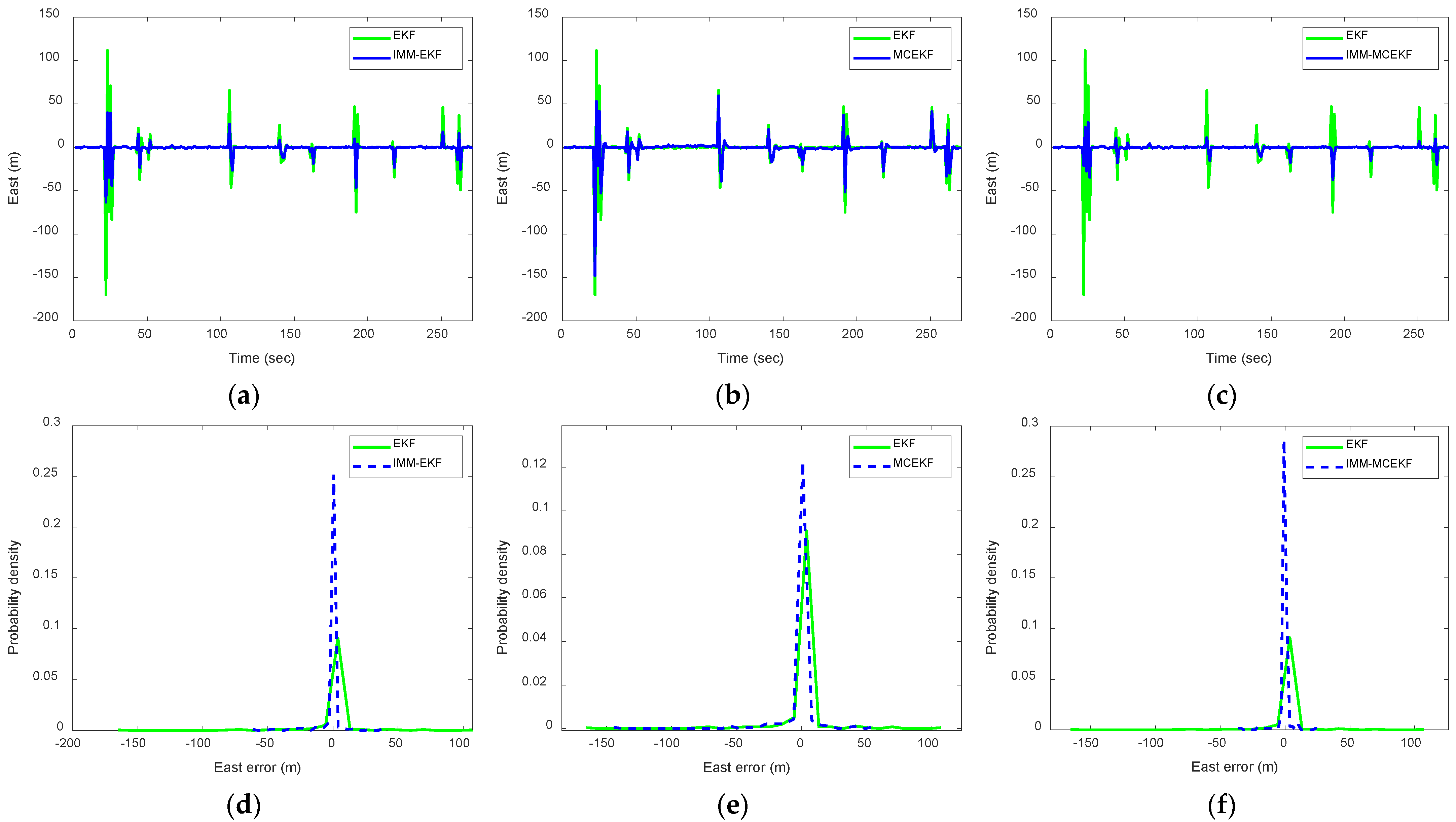
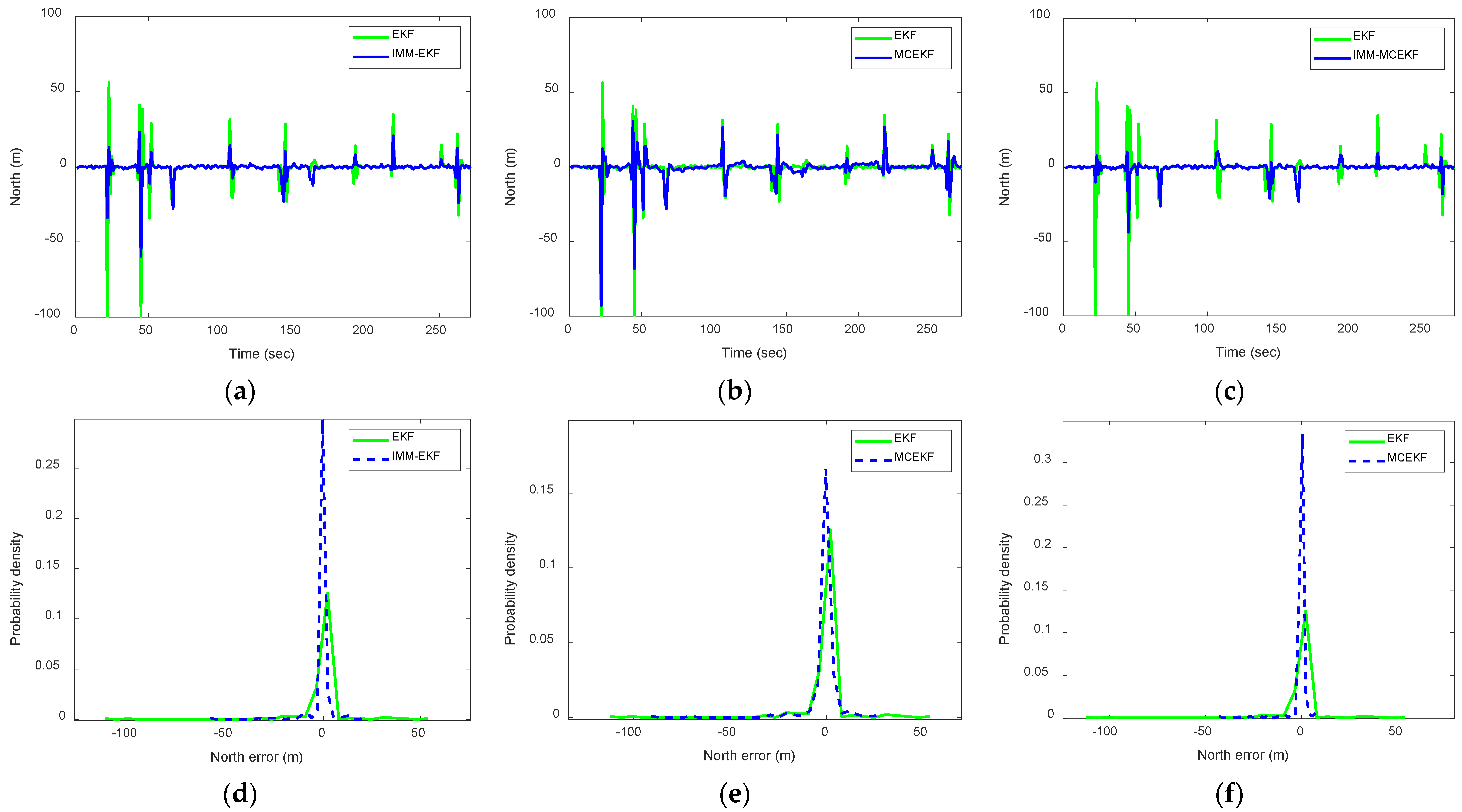
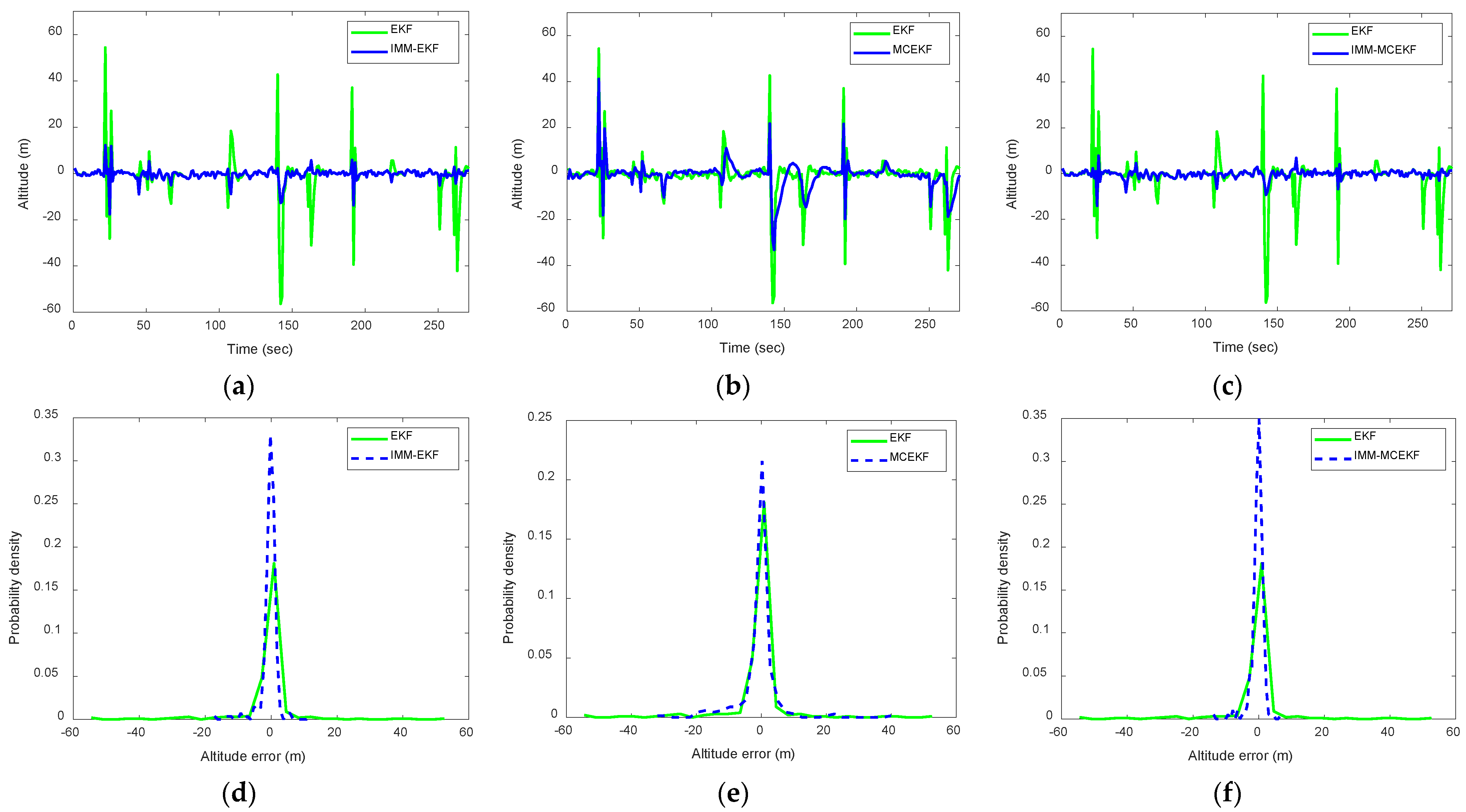
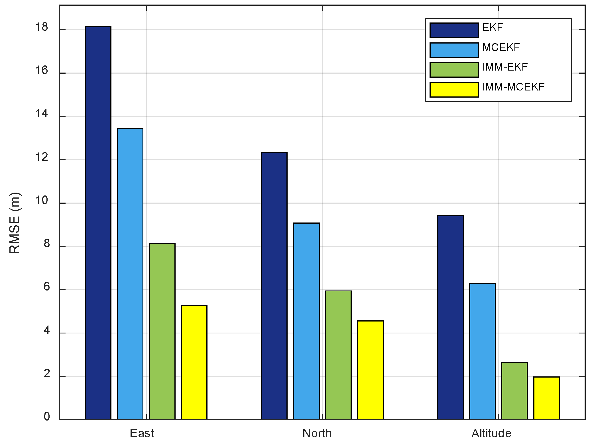
Figure 7, Figure 8 and Figure 9 present the results for all four filters (EKF, MCEKF, IMM–EKF, and IMM–MCEKF) based on 100 Monte Carlo simulation runs. We compared the corresponding pdfs of the position errors with the navigation accuracy for the different strategies. For a more specific comparison, the results for one of the East, North, and Altitude components are shown in each figure. Figure 10 is a clear representation of the pdfs from Figure 7, Figure 8 and Figure 9. It provides a comparison between the pdfs of three-dimensional position errors for the four approaches in the paper. Figure 11 compares the positional accuracy of the four approaches concerning the RMSE. Again, it can be seen that IMM–MCEKF shows a significant performance boost compared to the other three algorithms, although IMM–EKF and MCEKF each provide higher accuracy when used alone.

5. Conclusions

The multipath effect is one of the numerous interferences impairing GNSS positioning accuracy. Multipath-induced errors severely restrict the performance of high-precision GNSS receivers. Several estimation techniques were investigated for high-accuracy positioning systems since multipath mitigation is essential for enhancing positioning accuracy.

The KF algorithm was first constructed based on the minimal mean square error criterion, which is only optimal when the system is assumed to be linear and the noise to be Gaussian. However, the original EKF-based state estimation issue lacks adequate resilience when the system experiences non-Gaussian errors, making it impossible to estimate the state vector accurately. Therefore, alternative optimization criteria were proposed to replace MMSE to reduce the impact of non-Gaussianity and successfully solve the estimation issue when the system is subjected to such conditions. Using an ITL approach for non-Gaussian signal processing in GNSS navigation state estimation, MCC was devised because correntropy contains the second- and higher-order moments of errors. To address the estimating challenges in non-Gaussian noise situations, MCC was created to replace MMSE in a robust EKF called MCEKF.

This study proposed an extended Kalman filter with maximum correntropy criteria for processing GPS navigation, which is particularly helpful for minimizing the outlier type of multipath interference. Due to the alteration in observation data, the typical EKF cannot adjust the covariance parameters in the measurement model. Therefore, to further increase the accuracy in navigation state estimation, IMM was utilized to alter the covariance parameters of the measurement noises used in each of the parallel filters in the IMM architecture. The suggested IMM–MCEKF algorithm demonstrated a notable improvement in estimation accuracy and can act as a viable replacement for GNSS navigational processing based on performance comparisons with EKF, IMM–EKF, and MCEKF.

References

1. Hofmann-Wellenhof, B.; Lichtenegger, H.; Wasle, E. GNSS—Global Navigation Satellite Systems, GPS, GLONASS, Galileo, and More; Springer: Vienna, Austria; New York, NY, USA, 2008. [Google Scholar]
2. Sunderhauf, N.; Obst, M.; Wanielik, G.; Protzel, P. Multipath Mitigation in GNSS-based Localization Using Robust Optimization. In Proceedings of the IEEE Intelligent Vehicles Symposium, Alcalá de Henares, Spain, 3–7 June 2012; pp. 784–789. [Google Scholar]
3. Brown, R.G.; Hwang, P.Y.C. Introduction to Random Signals and Applied Kalman Filtering; John Wiley & Sons: New York, NY, USA, 1997. [Google Scholar]
4. Mehra, R.K. On-line Identification of Linear Dynamic Systems with Applications to Kalman Filtering. IEEE Trans. Autom. Control 1970, AC-16, 12–21. [Google Scholar] [CrossRef]
5. Mohamed, A.H.; Schwarz, K.P. Adaptive Kalman Filtering for INS/GPS. J. Geod. 1999, 73, 193–203. [Google Scholar] [CrossRef]
6. Li, X.R.; Bar-Shalom, Y. Estimation with Applications to Tracking and Navigation; John Wiley & Sons: New York, NY, USA, 1993. [Google Scholar]
7. Jwo, D.J.; Chung, F.C.; Yu, K.L. GPS/INS Integration Accuracy Enhancement Using the Interacting Multiple Model Nonlinear Filters. J. Appl. Res. Technol. 2013, 11, 496–509. [Google Scholar] [CrossRef] [Green Version]
8. Kim, Y.S.; Hong, K.S. An IMM Algorithm for Tracking Maneuvering Vehicles in an Adaptive Cruise Control Environment. Int. J. Control Autom. Syst. 2004, 2, 310–318. [Google Scholar]
9. Lee, B.J.; Park, J.B.; Lee, H.J.; Joo, Y.H. Fuzzy-logic-based IMM Algorithm for Tracking a Manoeuvring Target. IEE Proc.-Radar Sonar Navig. 2005, 152, 16–22. [Google Scholar] [CrossRef]
10. Li, X.R.; Bar-Shalom, Y. Design of an Interacting Multiple Model Algorithm for Air Traffic Control Tracking. IEEE Trans. Control Syst. Technol. 1993, 1, 186–194. [Google Scholar] [CrossRef]
11. Lin, X.; Kirubarajan, T.; Bar-Shalom, Y.; Li, X. Enhanced Accuracy GPS Navigation Using the Interacting Multiple Model Estimator. In Proceedings of the IEEE Aerospace Conference, Montana, CA, USA, 10–17 March 2001; Volume 4, pp. 1911–1923. [Google Scholar]
12. Chen, G.; Harigae, M. Using IMM Adaptive Estimator in GPS Positioning. In Proceedings of the 40th SICE Annual Conference, SICE 2001, International Session Papers, Nagoya, Japan, 27–27 July 2001; pp. 25–27. [Google Scholar]
13. He, R.; Zheng, W.; Hu, B. Maximum Correntropy Criterion for Robust Face Recognition. IEEE Trans. Pattern Anal. Mach. Intell. 2011, 33, 1561–1586. [Google Scholar] [PubMed]
14. Liu, W.; Pokharel, P.P.; Principe, J.C. Correntropy: Properties and Applications in Non-Gaussian Signal Processing. IEEE Trans. Signal Process. 2007, 55, 5286–5298. [Google Scholar] [CrossRef]
15. Izanloo, R.; Fakoorian, S.A.; Yazdi, H.S.; Simon, D. Kalman Filtering Based on the Maximum Correntropy Criterion in the Presence of Non-Gaussian Noise. In Proceedings of the 2016 Annual Conference on Information Science and Systems (CISS), Princeton, NJ, USA, 16–18 March 2016. [Google Scholar]
16. Chen, B.; Liu, X.; Zhao, H.; Principe, J.C. Maximum Correntropy Kalman Filter. Automatica 2017, 76, 70–77. [Google Scholar] [CrossRef] [Green Version]
17. Zhang, Z.; Qiu, J.; Ma, W. Adaptive Extended Kalman Filter with Correntropy Loss for Robust Power System State Estimation. Entropy 2019, 21, 293. [Google Scholar] [CrossRef] [PubMed] [Green Version]
18. Liu, X.; Qu, H.; Zhao, H.; Chen, B. Extended Kalman Filter under Maximum Correntropy Criterion. In Proceedings of the IEEE International Joint Conference on Neural Networks (IJCNN), Vancouver, BC, Canada, 24–29 July 2016; pp. 1733–1737. [Google Scholar]
19. Liu, X.; Qu, H.; Zhao, J.; Yue, P.; Wang, M. Maximum Correntropy Unscented Kalman Filter for Spacecraft Relative State Estimation. Sensors 2016, 16, 1530. [Google Scholar] [CrossRef] [PubMed]
20. Yang, N.; Tian, W.; Jin, Z. An Interacting Multiple Model Particle Filter for Manoeuvring Target Location. Meas. Sci. Technol. 2006, 17, 1307–1311. [Google Scholar] [CrossRef]
21. Yi, S.; Zorzi, M. Robust Kalman Filtering Under Model Uncertainty: The Case of Degenerate Densities. IEEE Trans. Autom. Control 2022, 67, 3458–3471. [Google Scholar] [CrossRef]
22. Emanuele, A.; Gasparotto, F.; Guerra, G.; Zorzi, M. Robust Distributed Kalman Filtering: On the Choice of the Local Tolerance. Sensors 2020, 20, 3244. [Google Scholar] [CrossRef] [PubMed]
23. Shannon, C.E. A Mathematical Theory of Communication. Bell Syst. Tech. J. 1948, 27, 379–423. [Google Scholar] [CrossRef]
24. GPSoft LLC. Inertial Navigation System Toolbox 3.0 User’s Guide; GPSoft LLC: Athens, OH, USA, 2007. [Google Scholar]
25. GPSoft LLC. Satellite Navigation Toolbox 3.0 User’s Guide; GPSoft LLC: Athens, OH, USA, 2003. [Google Scholar]
Figure 1. Example of outdoor multipath interference.
Applsci 13 01782 g001
Figure 2. The block diagram of the IMM filter algorithm (one cycle with r models).
Applsci 13 01782 g002
Figure 3. Flow chart of the maximum correntropy-extended Kalman filter (MCEKF).
Applsci 13 01782 g003
Figure 4. Test trajectory for the simulated vehicle.
Applsci 13 01782 g004
Figure 5. (a) The skyplot and (b) the GDOP during the simulation interval.
Applsci 13 01782 g005
Figure 6. Information for the sequences of outlier interferences.
Applsci 13 01782 g006
Figure 7. Comparison between the navigational accuracy and the corresponding probability density functions (pdfs) of the east position errors: (top) navigational accuracies for EKF vs. (a) IMM–EKF, (b) MCEKF, and (c) IMM–MCEKF, and (bottom) pdfs of position errors for EKF vs. (d) IMM–EKF, (e) MCEKF, and (f) IMM–MCEKF.
Applsci 13 01782 g007
Figure 8. Comparison between the navigational accuracy and the corresponding pdfs of the north position errors: (top) navigational accuracies for EKF vs. (a) IMM–EKF, (b) MCEKF, and (c) IMM–MCEKF, and (bottom) pdfs of position errors for EKF vs. (d) IMM–EKF, (e) MCEKF, and (f) IMM–MCEKF.
Applsci 13 01782 g008
Figure 9. Comparison between the navigational accuracy and the corresponding pdfs of the altitude position errors: (top) navigational accuracies for EKF vs. (a) IMM–EKF, (b) MCEKF, and (c) IMM–MCEKF, and (bottom) pdfs of position errors for EKF vs. (d) IMM–EKF, (e) MCEKF, and (f) IMM–MCEKF.
Applsci 13 01782 g009
Figure 10. Comparison between the pdfs of three-dimensional position errors for the four approaches: (a) east; (b) north; and (c) altitude.
Applsci 13 01782 g010
Figure 11. Comparison of the position accuracies in terms of RMSE for the four approaches.
Applsci 13 01782 g011
Disclaimer/Publisher’s Note: The statements, opinions and data contained in all publications are solely those of the individual author(s) and contributor(s) and not of MDPI and/or the editor(s). MDPI and/or the editor(s) disclaim responsibility for any injury to people or property resulting from any ideas, methods, instructions or products referred to in the content.