1. Introduction
Sound waves, or noise emissions, are one of the pollutants that urban citizens are most concerned about [
1]. To identify, measure, and determine exposure to environmental noise, city rulers are developing data strategies to capture, transform, and analyze information using Internet of Things (IoT) and big data technologies.
European Directive 2002/49/EC aims to establish a common approach for the assessment and management of environmental noise in order to standardize procedures and metrics. The goal is to avoid, prevent, and reduce harmful effects, including annoyance, for citizens as a result of exposure to different noise sources [
2]. The directive specifically promotes agglomerations of people such as cities or clusters of cities to create strategic noise mapping (SNM) and then share the findings with the public. Additionally, the outcome of these noise maps has led to the formation of action plans for noise reduction in areas identified as having high noise exposure (noise exposure protection zones).
More recently, numerous large cities have begun to deploy Wireless Acoustic Sensor Networks (WASN), which are based on IoT technologies [
3], in order to gather noise data that can be analyzed and utilized to update SNM and action plans. These WASNs are usually made up of two different types of stations: fixed-location sensors for long-term monitoring, and temporal location sensors for short-term monitoring. The latter can take the form of temporarily deployed sensors, instrumented vehicles with an acoustic sensor together with a geopositioning system to locate the measurement, or regular sound measure devices known as sonometers [
4].
While fixed stations remain at one place all their lifetime, allowing the continuous monitoring of noise levels to identify trends and seasonality, temporal stations are placed in a particular site during an established period of time (minutes, hours, or days) to measure the acoustic soundfield by gathering short-term data.
To recognize environmental acoustic patterns or behaviors, using the average or median of noise indicators for the overall assessment period, generally at least one year, is recommended by the Directive [
2]. Therefore, short-term data are not usually considered due to the lack of capability to capture seasonality components such as holidays or weekends. After the analysis of previously enunciated long-term statistics, two principal types of environmental acoustic patterns are usually recognized: special regime areas and quiet areas. Special regime areas include locations where the noise indicator exceeds a high threshold, while quiet areas include locations where the noise indicator is below a low threshold. Although other patterns with complex behavior can exist, advanced statistical techniques are required to recognize them.
In a number of out prior works [
5,
6], we applied unsupervised learning techniques to group the nodes of a WASN in clusters with the same behavior and recognize complex patterns on this basis. These complex patterns can provide insights to city managers for establishing personalized strategies and defining new acoustic areas. In the current research, the application of a supervised machine learning technique, Artificial Neural Network (ANN), is proposed to predict the long-term acoustic behavior group to which a location belongs by means of short-term measurements. In this way, temporal stations can be used by city managers to identify the environmental acoustic pattern of a site, enhancing the value of the WASN and improving the SNM.
During last few years, machine learning algorithms have been considered in a number of studies involving environmental acoustic data captured by WASNs.
Many of the studies found in the literature use supervised machine learning approaches to analyze audio signals. In New York City, a comprehensive dataset [
7] of labeled audio recordings was generated utilizing a WASN [
8] for the design and assessment of machine learning techniques. This dataset was used to perform methods for both identification [
9] and categorization [
10] of acoustic scenes and events. Recently, a deep learning structure was created using this dataset [
11] to retrieve urban sound events such as car horns and human speech from multi-label audio recordings. In a European project called DYNAMAP [
12], multiple machine learning techniques were evaluated for detecting [
13,
14,
15,
16] abnormal noise sources such as birds, bikes, vehicles with heavy loads passing over rough surfaces, horn vehicle noise, music in a car or in the street, ambulance sirens, airplanes, thunder storms, etc., in order to eliminate events unrelated to road traffic noise and create a noise map. In addition to the previously mentioned methods, other techniques utilizing supervised machine learning have been utilized for classifying sound sources. Maijala et al. [
17] introduced a pattern classification algorithm that used Mel-frequency cepstral coefficients as features to determine the primary noise source in the acoustic environment. In this research, two types of supervised classifiers, namely, artificial neural networks with two hidden layers of 10, 30, 50, or 100 neurons and a Gaussian mixture model, were compared. Ye et al. [
18] introduced an aggregation scheme combining local features and short-term sound recording features with long-term descriptive statistics to create a deep convolutional neural network for classifying urban sound events.
Regarding machine learning techniques for sound pressure level and acoustic pattern prediction, a number of studies have been published within the last few years. Das et al. [
19,
20] proposed an ANN architecture with only one hidden layer to predict annoyance levels of traffic noise. The architecture complexity of the trained ANNs (see
Section 2.4 for details about this definition) were
, with six variables in the input layer for the first study and
,
,
,
,
with five variables in the input layer for the second study. By utilizing short-term data and concentrating on traffic noise, unsupervised machine learning techniques such as dimensionality reduction and clustering were employed to optimize the location and quantity of monitoring sites [
21]. A separate publication [
22] presented a methodology for more efficiently estimating day-period and night-period sound pressure levels on urban roads in Milan, Italy in comparison to the legislative road classification by using equivalent sound pressure levels of a 1-h period from a 24 h measurement campaign. Subsequently, in order to link each street in the area of examination to one of the two noise profiles found through clustering, several non-acoustic parameters were examined [
22]. In another recent study, the intermittency ratio indicator was paired with the equivalent sound pressure level of a 1-h time frame in order to improve the categorization of different types of streets within the two identified clusters [
23].
Regarding the identification of the long-term environmental acoustic pattern of a city, Torija et al. [
24] investigated the necessary stabilization time, short-term variability, and impulsiveness of the sound pressure level to accurately characterize the temporal composition of urban soundscapes. The authors used data from sound level meters to analyze sound pressure levels in urban environments, and found that a stabilization time of at least 30 min was required to obtain reliable measurements of sound pressure level. The same study suggested that measurements should be taken over a longer period of time to achieve a more accurate characterization of urban soundscapes, and that the short-term variability and impulsiveness of sound pressure levels should be considered as well. In a later study, Gajardo et al. [
25] analyzed data collected from sound level meters in various urban environments and concluded that hourly averages of sound levels may not be representative of the true levels of noise exposure. Therefore, using longer measurement periods such as 24 h, to obtain more accurate representation of noise levels in urban environments was recommended. On the other hand, regarding the prediction of the equivalent sound level using short-term measurements, Brambilla et al. [
26] focused on the stabilization time for road traffic noise measurements and concluded that a time of at least 10 min is necessary for reliable estimation of the equivalent sound pressure level of 1-h period; in addition, factors such as traffic volume, traffic composition, and road type can affect the required stabilization time.
An environmental acoustic pattern refers to the distribution and variation of sound levels in a specific environment. These patterns can be affected by a variety of factors, such as land use, weather conditions, and human activity. In urban environments, the environmental acoustic pattern is typically characterized by high levels of noise pollution from sources such as traffic, construction, and industrial activities. However, these noise sources create a complex and dynamic acoustic environment which is highly dependent on the time of day and location. In this research, the environmental acoustic pattern of a location refers to the classification of a location using the equivalent sound pressure level during the day, evening, and night periods over a year, as recommended by the Directive [
2] and defined in
Section 2.2.
The contribution of the current research is to use an unsupervised learning algorithm to estimate the corresponding environmental acoustic pattern of a location among the recognized long-term behaviors based on one-year acoustic data. This is carried out by using one-hour equivalent acoustic data to design and test algorithms based on ANNs, which are trained using shorter periods of time with a large amount of available data and require parallel processing to optimize the data pipelines.
This rest of this paper is structured as follows. The datasets, algorithms, and methodology used for training and testing the models are presented in
Section 2. Then, in
Section 3, the results obtained from the analysis are displayed and discussed. Finally,
Section 4 summarizes the main conclusions of this work.
2. Materials and Methods
In this section, the materials and methods applied during this research are presented. The data source containing the sound pressure level values of the sites and the collection methodology are described in
Section 2.1. The environmental acoustic patterns recognized in a previous work [
5] are summarized in
Section 2.2. Next, the curated short-term datasets used in this research and their transformations are detailed in
Section 2.3.
Section 2.4 presents the machine learning models that have been trained and evaluated in this work. Finally, the metrics used in the evaluation of the models are defined in
Section 2.5.
The data preparation, transformation, analysis, modeling, and visualization were executed utilizing the Statistical Programming Language R [
27], which involved the integration of a local environment using R version 4.2.1 with a free cloud-based environment provided by Posit Cloud using R version 4.2.2. The scripts applied in this research are available at the Github repository
https://github.com/AntonioPL/BCN_Noise (accessed on 6 January 2023). In order to ensure the reproducibility of the research, the seed was fixed using the R function set.seed() in every task that incorporated a random step.
2.1. Data Source
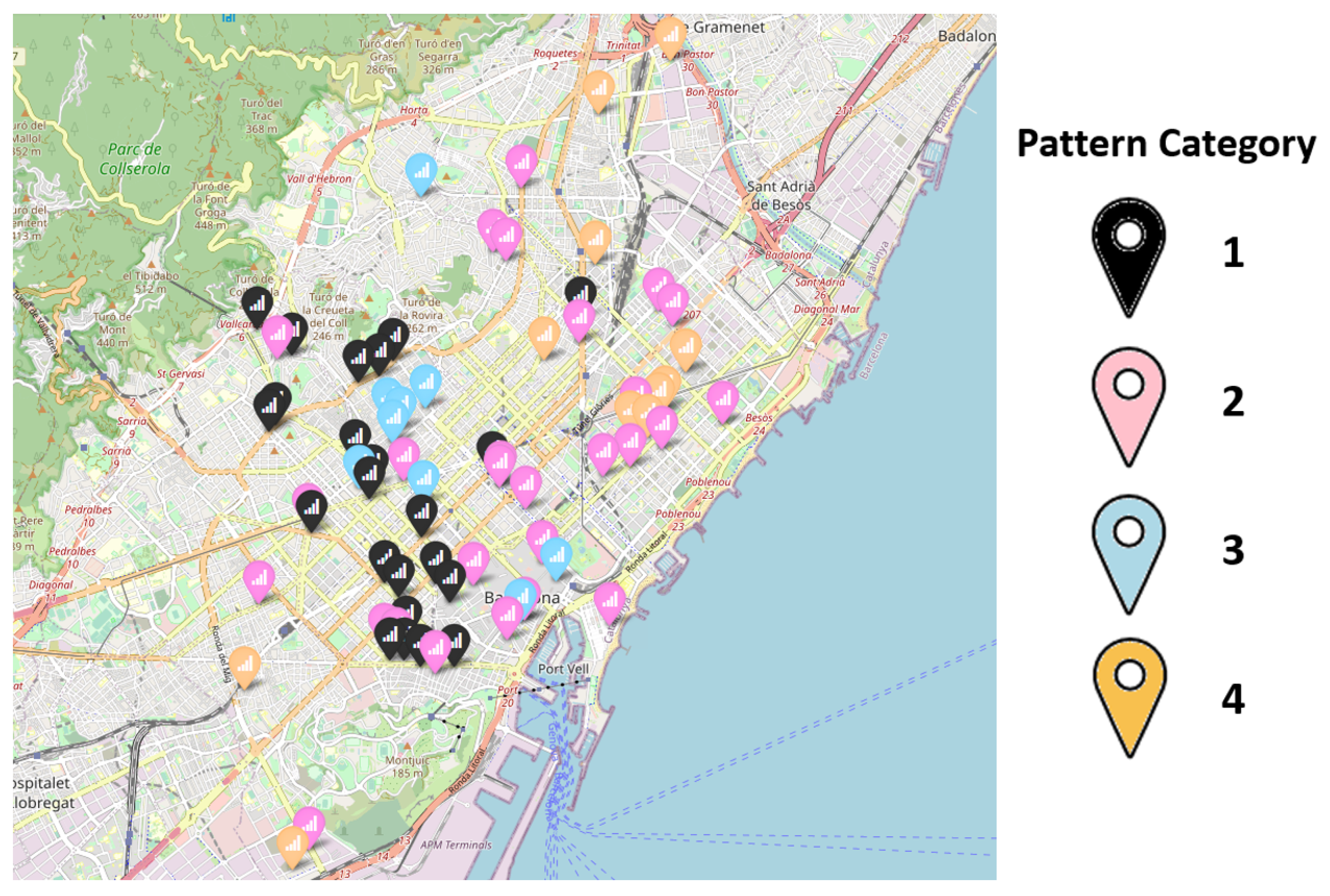
The historical data used in this research contain sound pressure level values from 70 fixed acoustic nodes deployed in Barcelona, Spain, to build a WASN, as described in publications by Camps et al. [
28] and Farres et al. [
29]. The map in
Figure 1 shows the widespread distribution of the nodes in the whole city.
These fixed acoustic nodes are equipped with remote Cesva TA120 [
30] sonometers, which capture sound pressure levels continuously 24 × 7 (24 h and 7 days a week) and every minute send the A-frequency weighting equivalent sound pressure level of a 1-min period, denoted as
, as defined in Equation (
1) following ISO1996-2 [
31]:
where
is a 1-min interval beginning at time
,
is the sound pressure level at time
t in Pascal pressure units (
), and
is the sound pressure reference value.
These data are captured every minute and stored in the central data storage [
28], where transformation are performed before the data are absorbed into the smart city platform of BCN called Plataforma de Sensors i Actuadors de Barcelona [
32].
More than 97 million of
records captured by BCN city council in the full years from 2018 to 2020 for the 70 nodes were exported from the smart city platform in 73 Excel
™ files with wide data format for use in this research. These files contain sound pressure level values of every minute for every node in the described period. It is worth noting that there were a number of null values due to sensor errors and maintenance periods; these were removed during the curation phase. Basic statistics and available records from the nodes can be found in [
5].
2.2. Environmental Acoustic Patterns
To evaluate the environmental acoustic behavior of a site, European Directive 2002/49/EC [
2] recommends the use of the
indicators corresponding to day, evening, and night periods over 24 h for a specific station on every day during one year, denoted as
,
and
, respectively, and the overall assessment period noise indicator DEN (day, evening, night), represented by
. To take into account the temporal variability of the sound pressure level values during the different periods of the day, the yearly standard deviation of
, denoted
(
), has been proposed to describe the variability or volatility of the sound pressure level of the nodes during a year [
5,
6]. In these previous works of ours, four environmental acoustic patterns were recognized using these four noise indicators, calculated from the described dataset as inputs of several unsupervised learning techniques. Therefore, the nodes of BCN’s WASN were classified into one of these patterns, and are shown in
Figure 1 in different colors together with their locations.
Table 1 shows the average values of the four previously defined noise indicators for the different pattern categories that allow the description of their behaviours. Analytically, there are three pattern categories in which day and evening sound pressure level values are similar and in which both are higher than night sound pressure level values by a statistical significance amount. The first pattern category, shown by the 23 nodes with the black color tag in
Figure 1, has higher sound pressure values (
,
and
) than the second pattern category, shown by the 27 nodes with the magenta color tag in
Figure 1. Both categories have higher sound pressure values than the fourth category, which includes the 11 nodes shown with the brown color tag in
Figure 1. Therefore, these pattern categories represent nodes with high, medium, and low values of sound pressure with the described behavior. Moreover, a negative correlation between sound pressure levels indicators and variability (
(
)) can be observed, i.e., the fourth category is the one with the highest variability, followed by the second and first categories, in this order. The remaining third category, indicated by the blue color tag, contains nine nodes. This category shows a different behavior than the others, with evening sound pressure level value being higher than the other periods, which all have similar values. Moreover, this third category presents the highest variability of all categories.
These environmental acoustic patterns can be contextualized by features such as the type of roads, use of the area, and noise sources. Interpretation of these characteristics allows for a deeper understanding and appreciation of the behavior patterns of different city areas. This can be valuable for residents, tourists, businesses, and city managers.
Behavior Category 1 groups the locations related to main routes of road traffic, in particular, major thoroughfares and intersections with very high road traffic intensity. Noise levels are relatively consistent during the day, with peak noise levels occurring during rush hour when traffic is heaviest. At night, noise levels decrease somewhat due to reduced traffic volume, though they are still significantly higher than in quiet residential areas. The sound pressure level is high and fluctuation is low, as shown in
Table 1.
Behavior Category 2 groups those locations related to the regular areas in a city, which typically include medium-density residential, commercial, and office building areas along with public spaces such as parks, squares, and sidewalks. The noise pollution is moderate to high, with a wide range of noise sources. During the day the noise level is relatively consistent, with peak noise levels occurring during peak hours of activity such as rush hour and lunchtime. At night, noise levels decrease somewhat due to reduced activity, though they remain higher than in quiet residential areas. In this category, the sound pressure level is moderate to high and the fluctuation is moderate, as shown in
Table 1.
Behavior Category 3 groups the locations related to shopping, entertainment, and nightlife activity. The noise pollution is high throughout the day, evening, and night due to the high level of human activity and mix of commercial and entertainment venues. During the day, noise levels are high and relatively consistent, with peak noise levels occurring during peak hours of shopping and entertainment activity. In the evening, noise levels continue to be high, and are more fluctuating, with an increase in human activity as people go out for entertainment and nightlife. At night, noise levels are high and fluctuating, with an increase in human activity in nightlife venues such as bars, clubs, and restaurants. In this category, both the sound pressure level and fluctuation are high, as is shown in
Table 1.
Finally, Behavior category 4 is related to quiet residential areas in a city, where the noise pollution is low during the day, evening, and night periods. These areas are characterized by lower levels of human activity and fewer noise sources, providing a relatively peaceful and quiet environment for residents. Noise levels are low during the day, with occasional spikes from passing vehicles and aircraft or distant construction and maintenance work. In the evening noise levels decrease even further due to lower traffic and other human activities. Noise levels at night decrease significantly, as expected. However, occasional high noise level events, e.g., from passing vehicles or aircraft, can explain the elevated fluctuation of the sound pressure level shown in
Table 1.
In the current research, short-period measurement data are used to estimate the corresponding behavior recognized using long-term data, i.e., the environmental acoustic pattern category is the output variable of the proposed supervised learning algorithm.
2.3. Curated Modelling Datasets
To train and evaluate the machine learning models, 24 short-term period curated datasets were prepared and denoted using numbers from 0 to 23, sequentially corresponding with every one-hour time slot of the day. Each instance contains 60 sound pressure level values for a particular node on a specific date at the fixed hour, i.e., dataset number X contains all the sound pressure level values captured from X:00 until X:59 in hh:mm format for every node at any date from January 2018 until December 2020.
Table 2 shows the distribution of these 24 datasets, detailing the amount of available, valid, and null instances and the average instances per node for every dataset. As a summary, there are 1,621,145 valid instances, which is 93.66% of the total available instances, with an average of 23,159 instances per node.
The following tasks were applied to these curated datasets to train and test the models implemented with the machine learning technique described in
Section 2.4. First, instances with null values were removed. Then, every dataset was randomly split into two subsets, called the training and and test sets. The training subset contained 80% of the curated dataset instances, and was the input for model training, while the test subset contained 20% of the curated dataset instances, and was used to evaluate the models.
2.4. Artificial Neural Networks
To estimate the target variable or pattern category described in
Section 2.2 using the curated datasets described in
Section 2.3, supervised learning algorithms were considered. In particular, several feed-forward multilayer Artificial Neural Networks were built.
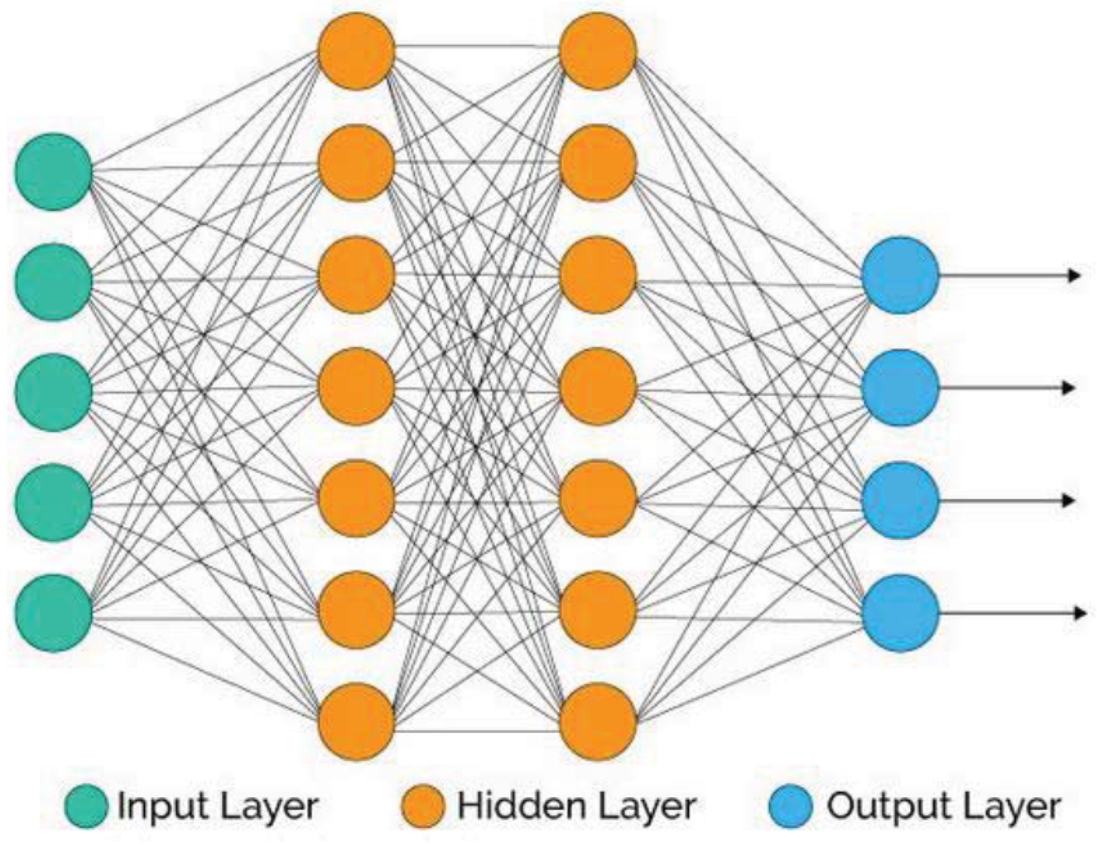
A feed-forward multilayer ANN is a mathematical model composed of elements called neurons [
33] grouped by layers and relationships between the elements of a layer with the elements of the previous layer by activation functions, as displayed in
Figure 2.
There are three different types of layers, as can be seen in
Figure 2. The input layer, represented by the green circles, is fed the input dataset, meaning that the size of this layer must be equal to the size of every instance in the dataset (60 in this work). The output layer, represented by the blue circles, is populated by the output variable to be estimated, meaning that the size must match the number of categories described in
Section 2.2 (four in this work). Moreover, there are one or more intermediate layers, usually known as hidden layers, which are represented by the orange circles in
Figure 2. The hidden layers can have different sizes. To fit the parameters of these layers to the data, a backpropagation algorithm [
35] was used, with normalized exponential (softmax) as the activation function of the output layer and rectified linear unit (ReLU) as the activation function of the hidden layers.
In this article, the notation
represents a feed-forward ANN architecture with
n hidden layers with size
for hidden layer
i and size
Y for the output layer. In particular, eight architectures with a different number of hidden layers and different amounts of neurons in the layers were trained on the 24 datasets described in
Section 2.1, resulting in 192 models used in the comparison. The eight detailed architectures are the following:
,
,
,
,
,
,
, and
. Note that all the models have four neurons in the output layer.
2.5. Performance Metrics
In this study, the classification performance of the trained models was measured globally and for each category using three different metrics: Accuracy, F1-Score, and Balanced Accuracy.
Accuracy, the percentage of elements correctly labeled by the model, was calculated using Equation (
2) to evaluate the global performance of the models:
where
N is the quantity of elements,
C is the number of categories, and
is the quantity of elements belonging to real category
i correctly labeled by the model as category
i for every category
i. By definition, the Accuracy is a real number between 0 and 1. A high Accuracy indicates good global performance of the model, with the best result reaching 1 when all the elements are correctly labeled by the model.
On the other hand, F1-Score and Balanced Accuracy were calculated for every category
i to evaluate the performance of the model over every category. Thr F1-Score is the harmonic mean of the trade-off metrics, precision and recall, as defined in Equation (
3), for every category
i:
where
is the quantity of elements belonging to real category i incorrectly labeled by the model as a category different from i, while is the quantity of elements not belonging to real category i incorrectly labeled by the model as category i. The maximum possible F1-score value is 1, which indicates perfect precision and recall, while the minimum possible value is 0, which is the case if either precision or recall is zero.
Second, Balanced Accuracy is the arithmetical mean of the trade-off metrics, sensitivity and specificity, as shown in Equation (
6):
where
and
is the quantity of elements belonging to real category
i incorrectly labeled by the model as belonging to a category other than
i. The highest possible Balanced Accuracy value is 1, indicating perfect Sensitivity and Specificity, and the lowest possible value is 0, which is the case if both Sensitivity and Specificity are zero.
In summary, when evaluating a particular category, the closer the Balanced Accuracy and F1-Score are to 1, the better the model can correctly classify observations.
3. Results and Discussion
This section presents and discusses the results obtained in the comparison between trained models for the different ANN architectures. This evaluation was carried out in three approaches: global performance, time slot, and environmental acoustic pattern.
First, the performance of the different models on the test datasets was calculated using Accuracy as a global metric.
Table 3 shows the Accuracy of the 192 trained models for the eight ANNs defined in
Section 2.4 on the test subsets of the 24 datasets representing each hourly time slot, where time slot
X corresponds to the interval from X:00 hour to X:59 hour, as defined in
Section 2.3.
The global performance of the models depends on the time slot and the model, as expected; , from 21:00 to 21:59, shows the highest Accuracy at 0.6943, resulting in the best combination of architecture and hourly time slot. This is a particular insight, very valuable for city managers; however, this asseveration is difficult to generalize for other cities. Analyzing these results, a discussion is provided in the following paragraphs in order to obtain more general conclusions.
Due to the existence of four categories, adopting a random model supposes an Accuracy of 0.25 in each of them. As shown in
Table 3, in general, all models across every hour exceed the random model except one. As the pattern categories are not equally distributed (see
Table 1), a baseline model could be the selection of the most representative category with an Accuracy of 0.39 (=27/70). Even though the Accuracy of the models ranges from 0.150 to 0.694, 160 of the 192 models (83%) have an Accuracy higher than the baseline model. In addition, a one-sided parametric hypotheses testing was carried out with the hypotheses represented in Equation (
9):
Considering the central limit theorem, the test statistic follows a Student’s t-distribution with 191 degrees of freedom, and the estimator of the test is 18.929, equivalent to a . Therefore, the null hypothesis is rejected, leading to the conclusion that the improvement when using an ANN to estimate the long-term environmental acoustic pattern of a spot based on short-term data is statistically significant.
Regarding the optimum hourly time slot to capture data that best represent the long-term pattern,
Table 3 shows that on average every hourly time slot improves the baseline model; the better hourly time slots to predict environmental acoustic behaviors are 14, 17, 20, 4, and 21, in which the averaged Accuracy is higher than 0.55. Finally, the worst time slots to capture data are 7, 10, 8, 12, 22, and 11, in which the Accuracy is lower than 0.49.
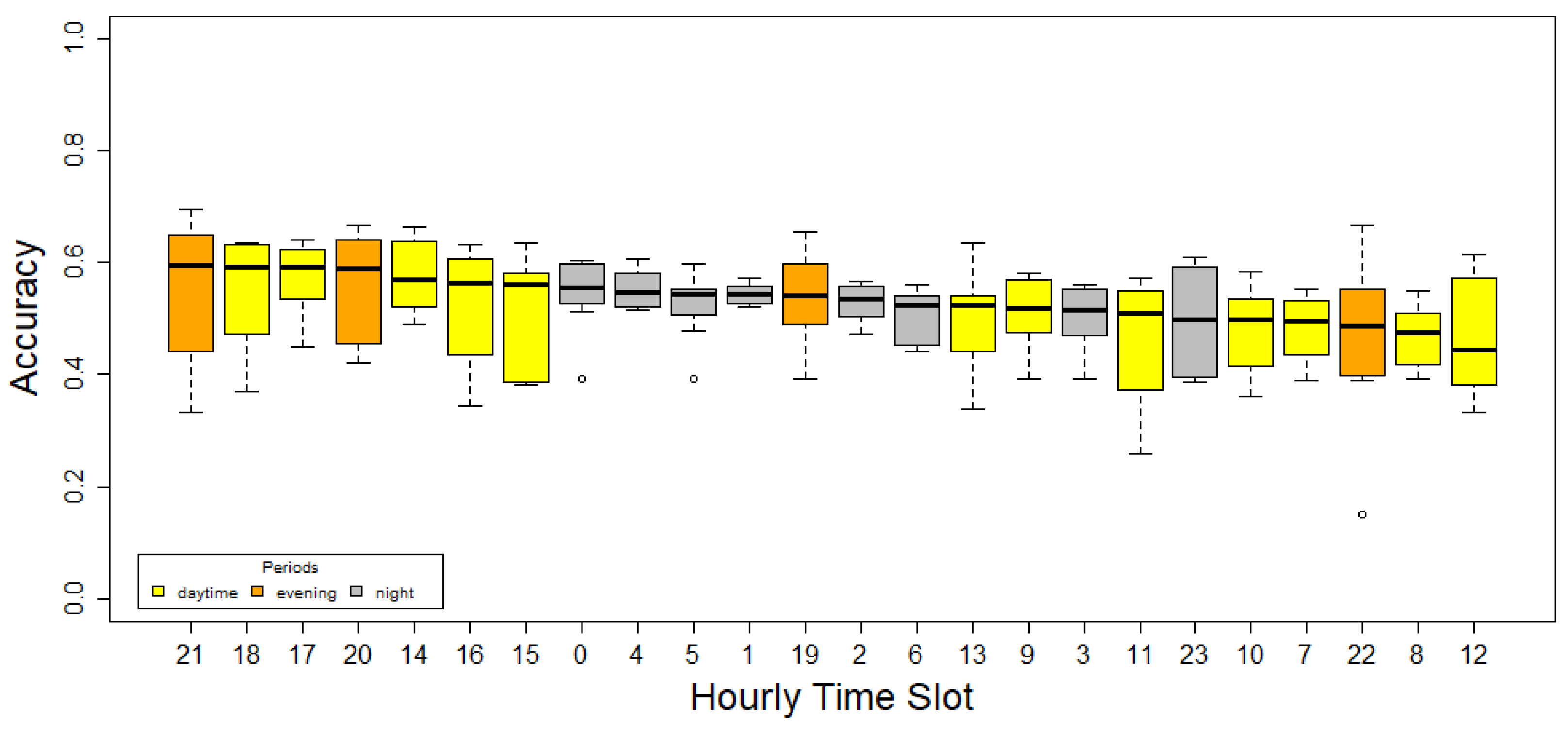
However, outliers decrease the representativeness of the mean value. Therefore, a median Accuracy analysis was performed to minimize the impact of outliers in the above results. The Accuracy distribution for each hourly time slot ordered by the median of the Accuracy is shown in
Figure 3. These hourly time slots are colored yellow for daytime periods (from 7:00 a.m. to 7:00 p.m.), orange for evening periods (from 7:00 p.m. to 11:00 p.m.), and gray for night periods (from 11:00 p.m. to 07:00 a.m.), as defined in Directive 2002/49/EC [
2].
Figure 3 shows that 21, 18, and 17 are the best hourly time slots, in this order. On the other hand, the worst time slots are 22, 8, and 12. The top seven most accurate hourly time slots are in the interval 14 to 21. From this interval, only 19 is not in the ranking, falling to the twelfth position. Therefore, the period from 14:00 to 22:00 is recommended to capture data and estimate the location acoustic pattern.
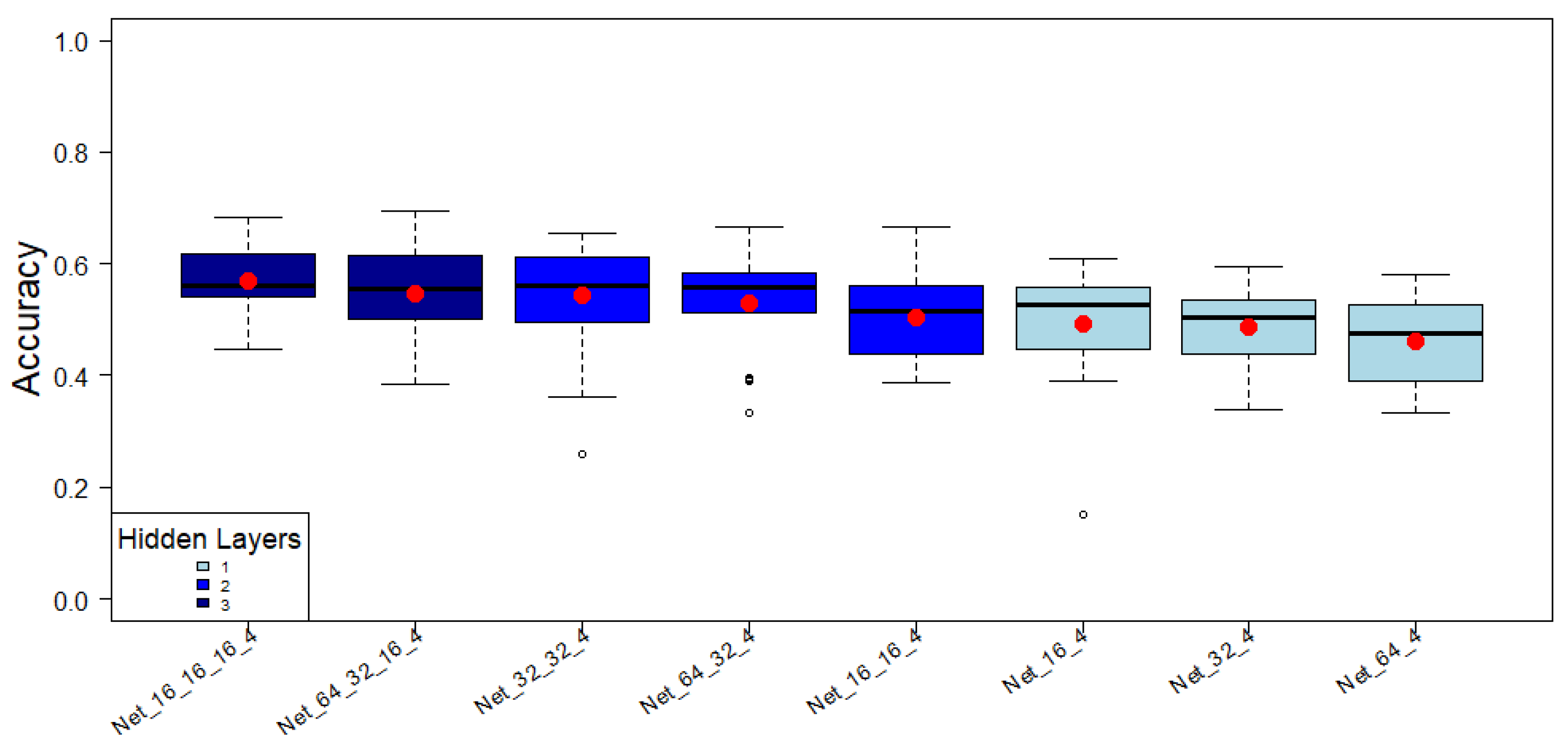
Next, the impact of the complexity of the ANN architecture on the performance in the classification was analyzed.
Figure 4 shows a comparison of the distribution of the Accuracy performance metric. The fill color represents the number of hidden layers, with light blue, blue, and dark blue standing for 1, 2, and 3, respectively. Although the models with a higher quantity of hidden layers have the highest average Accuracy, the amount of neurons in the layers does not significantly affect Accuracy.
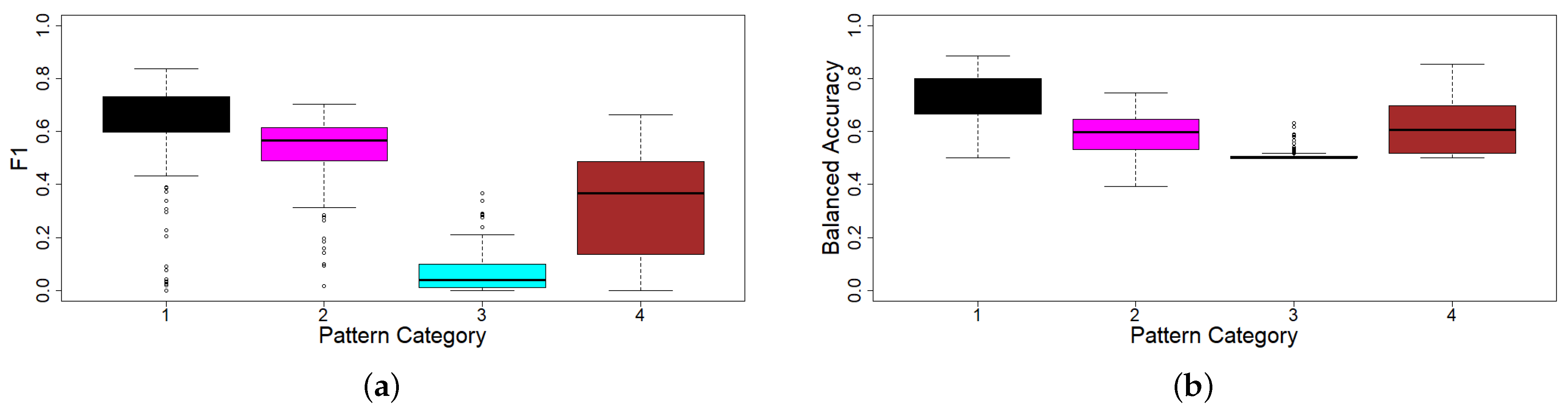
Finally, the performance of the models in relation to each pattern category, as described in
Section 2.2, was evaluated using Balanced Accuracy and F1-score.
Figure 5 shows that Pattern Category 1 has the best performance on average (0.63 F1-Score and 0.75 Balanced Accuracy), followed by Categories 2 (0.53 F1-Score and 0.59 Balanced Accuracy) and 4 (0.32 F1-Score and 0.60 Balanced Accuracy). Category 3 is the most difficult to predict (0.07 F1-Score and 0.50 Balanced Accuracy). This observation is inverse correlated with the
(
) of each pattern category, meaning that its higher the volatility makes this category harder to predict. It is important to note that one-hour time slots are used as a short-term measurement period; thus, improvements in the predictions for Pattern Category 3 can be achieved by combining data from two or more hourly time slots.
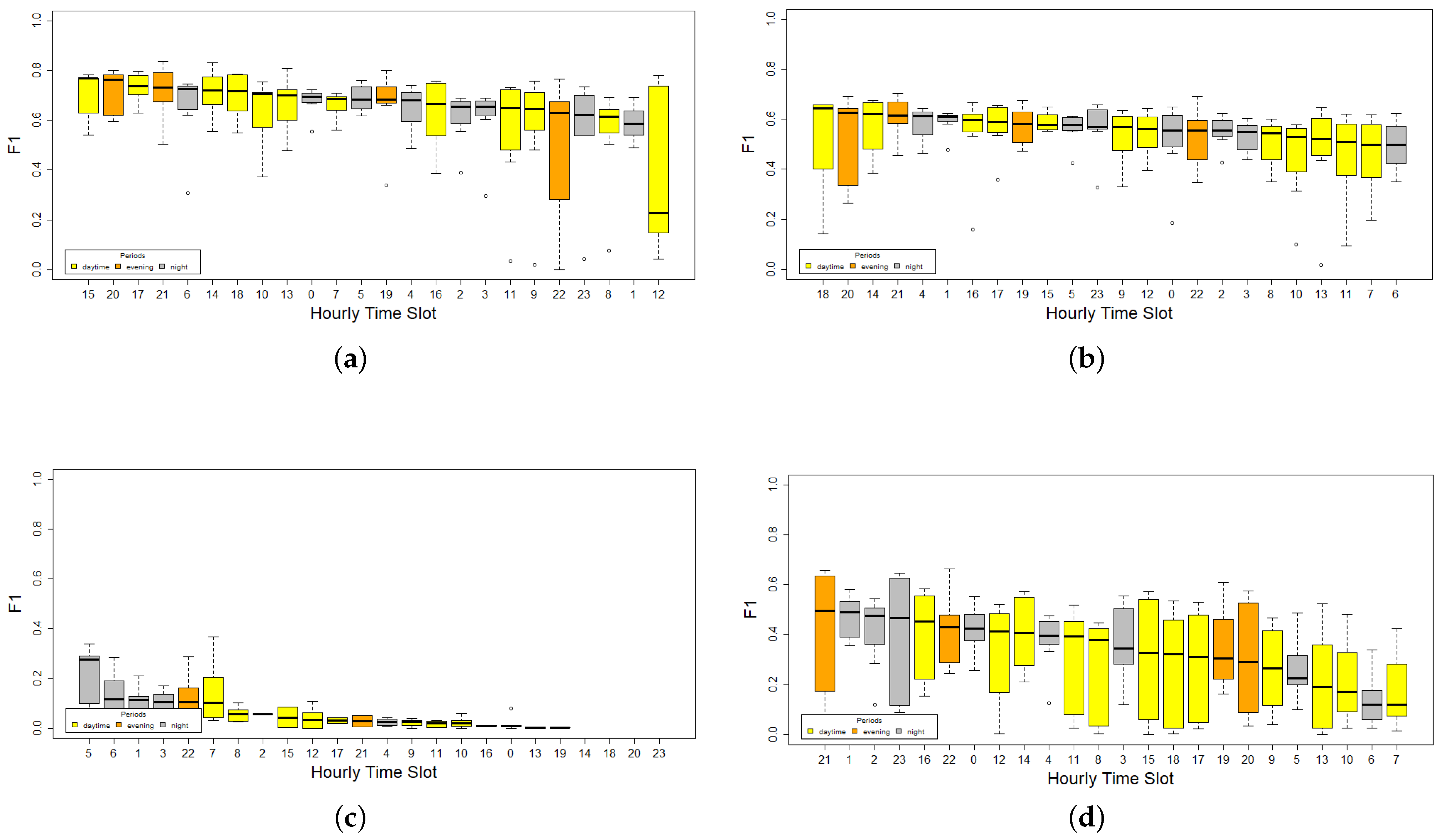
To obtain further insights into the prediction ability, an hourly time slot F1-Score performance comparison was carried out for every category.
Figure 6 shows similar trends in Categories 1 and 2 regarding median F1-Score for each hourly time slot. Most of these have low variability, meaning that in general any period could be used to predict these environmental pattern categories. On the contrary, Category 3 has low performance at all time slots, improving in the nightly period, but not enough to be confident in the prediction. Therefore, other strategies, for example, increasing the size of the time period or including several hourly time slots as input data, should be considered in future works. Finally, Category 4 presents a wide range of performance values, highlighting the nightly period 21:00–02:00 as the best period. Moreover, the variability of the F1-Score distribution for Category 4 is the highest of all categories.
4. Conclusions
In this paper, we carried out an evaluation of the suitability of predicting the long-term environmental acoustic pattern of a position based on information collected in a short-term interval using artificial neural networks. For this, we used a dataset with sound pressure level values from the city of Barcelona, Spain, captured with a wireless acoustic sensor network. Using several performance metrics, we performed a comparison between 192 models designed with eight different architectures and trained using hourly sound pressure level datasets.
In general, the results show that artificial neural networks can classify short-term acoustic data into one of several recognized long-term environmental acoustic patterns. From a global perspective, models with higher quantity of hidden layers have better performance, even though this performance is not affected by the amount of neurons, and the performance increases if the data are gathered in an hourly time slot included in the interval from 14:00 to 22:00. Regarding particular environmental acoustic patterns, those with lower sound pressure level variability are easier to estimate using hourly sound pressure level measurements.
The provided insights are crucial to define the data collection methodology in order to assure the most accurate pattern category prediction and avoid bias created by stable routines with temporal stations. Moreover, it is recommended to capture data at the same time slot in different locations, as this improves recognition of the specific environmental acoustic behavior of a place.


