Article

A Comparison between Two Statistical Methods for Gear Tooth Root Bending Strength Estimation Starting from Pulsator Data

1
Politecnico di Milano, Dipartimento di Meccanica, Via La Masa 1, 20156 Milano, Italy
2
Gear Research Center (FZG), Technical University of Munich, 85748 Garching bei München, Germany
*
Author to whom correspondence should be addressed.
Appl. Sci. 2023, 13(3), 1546; https://doi.org/10.3390/app13031546
Submission received: 9 December 2022 / Revised: 17 January 2023 / Accepted: 20 January 2023 / Published: 25 January 2023
(This article belongs to the Special Issue Modern Research of Gears and Power Transmission)

Abstract

:
Due to their cost-effectiveness, pulsator tests are widely adopted as a testing methodology for the investigation of the effects of material and heat and surface treatment on the gear strength with respect to tooth root fatigue fracture. However, since no meshing contact is present in pulsator tests, there are differences between the test case and the real-world application scenario where gears are rotating under load. Those differences are related to both statistical and fatigue phenomena. Over the years, several methodologies have been developed in order to handle this problem. This article summarizes them and proposes a first comparison. However, no complete comparison between the different estimation methodologies has been conducted so far. This article aims to partially cover this gap, first by presenting and comparing the methodologies proposed in the literature and then via a deeper comparison between two different elaboration methodologies. Those two methodologies, which have been developed by examined to the same test rig configuration, are also discussed in detail. The comparison is performed based on an actual database composed of 1643 data points from case-hardened gears, divided into 76 experimental campaigns. Good agreement between the estimated gear strengths was found. The database is also adopted in order to make further considerations about one methodology, providing additional validation and defining the specimen numerosity required.

1. Introduction

Gears are machine elements that, as a result of the meshing of their profiles, allow the transmission of power between two rotary axes while maintaining a (nominal) constant ratio between the rotational velocity of the two axes [1,2,3]. Their working principle implies the presence of a loaded sliding/rolling contact condition that is located far from the base of the tooth (i.e., the tooth root). The contact implies the co-presence of several failure modes, such as tribological damages (i.e., scuffing and wear) and fatigue damages (e.g., (macro)pitting, micropitting, tooth flank fracture, and tooth root fatigue fracture). The latter (also called tooth root bending fatigue or tooth root breakage) is related to the pulsating normal force that acts on the tooth flanks, which causes a bending stress history in the tooth root that starts from a small negative value (when the previous tooth pair is in mesh) up to a maximum (ideally when the contact is at the outer point of the single tooth contact) [4,5]. Furthermore, the root radius works as a notch, further increasing the maximum stress [5]. Amongst all the failures that can affect a gear, tooth root fatigue fracture is considered to be the most critical one. Indeed, the failure of a single tooth implies the stoppage of the power flow within the gearbox and typically leads to a total failure of the gear system.
Fortunately, standards such as ISO 6336-3 [6] and ANSI AGMA 2001-D04 [7] provide gear designers with standardized analytical tools that can be used to assess a gear pair with respect to this failure mode. The assessment is based on the comparison of the occurring tooth root stress with the permissible tooth root stress. The first is primarily based on the maximum tensile stress at the surface in the tooth root fillet, typically for external gears at the 30° tangent, and depends on the gear pair meshing characteristics and the tooth root shape. The latter is based on typical gear material (together with the treatments) strength data and is defined at 1% gear failure probability. Typical resistance data are also part of these standards (i.e., [7,8]).
However, due to their intrinsic limitations, the standards cannot cover all possible varieties of materials and (heat or surface) treatments. Moreover, as Figure 1 shows, even the standards do not provide a comprehensive gear SN curve but rather a scattering range (see the shaded area) for > 3 10 6 load cycles, leaving the designer to assume strength in the long-life region. Indeed, the standards themself strongly recommend performing experimental campaigns to properly estimate the gear load-carrying capacity.
Three main testing methodologies for tooth root fatigue fracture are present in the literature: The Meshing Gear (MG) test (e.g., [9]), the pulsator test (e.g., [10,11,12,13,14,15]), also known as the Single Tooth/Teeth Bending Fatigue (STBF) test, and the test of notched specimens (e.g., [16,17,18,19,20]). The most common testing methodology is the pulsator test [21]; indeed, the tests are performed on a gear, rather than a notched specimen, while using a generic uniaxial testing machine, rather than a full gearbox. Therefore, pulsator testing is a cost-effective method that considers a representative test specimen. A description of the typical testing rig is presented in Section 2.
ISO 6336-5 [8] strength number data have been obtained based on both industrial experience and experimental investigations applying this kind of testing methodology. In this context, it is important to mention that although pulsator tests are part of the ISO 6336 series, the standard does not provide any indications about how to perform pulsator experimental campaigns and how to elaborate their outcome.
The fact that in pulsator tests, the teeth are loaded by anvils (clamping jaws) rather than by gear meshing, implies that there are some differences between the pulsator test and the real-world application scenario. Those differences are related to two main aspects:
  • From the fatigue point of view, the tooth root stress history is different. On the one hand, in pulsator tests, the stress trend is sinusoidal with R > 0. On the other hand, in the MG case, the tooth root stress presents a peculiar stress trend that is influenced by the load sharing between teeth pairs (and the related tooth deformability). This difference is typically solved by means of corrective coefficients that modify the SN curve (e.g., [22]).
  • From the statistical point of view, it must be considered that pulsator tests are performed on selected teeth rather than on the complete gears. Furthermore, not all teeth of a gear can be tested. Commonly, statistical tools are adopted here.
Pulsator tests are also affected by the typical difficulties of every fatigue experimental campaign, that is, the proper estimation of the experimental SN curve, both in terms of test planning and how to determine the SN curve while also taking into account the runouts (i.e., specimens that overcome the runout level, that is, the number of cycles after which the test is suspended).
To overcome all these difficulties, several methodologies have been proposed in the literature. However, no systematic and holistic comparison between the outcomes of different estimation methodologies has been made so far. This paper aims to partially cover this gap.
First, a comparison between methodologies is proposed here. Then, focusing only on the statistical aspect of the pulsator problem, a more detailed comparison between the two estimation methodologies is discussed. This is performed by examining the gear SN curves estimated starting from the pulsator test data. Those two methodologies were developed by examining a symmetric test configuration together with a specific emphasis on case-hardened gears. One method is currently adopted at FZG (Gear Research Center, in German: Forschungsstelle für Zahnräder und Getriebesysteme) and is described in [23,24,25,26]. The second one, instead, had been recently developed at Politecnico di Milano (POLIMI from now on) [27,28]. Both gear SN curve estimation methods have been developed by the authors.
Here, after a short presentation of the testing methodology (Section 2) and a literature review of how the literature deals with pulsator test data (Section 3), two estimation procedures are described deeply in Section 4 and Section 5. The comparison between the two methodologies was performed based on the case-hardened gears experimental database presented in Section 6. The comparison is reported in Section 7. In Section 8, the adopted database is used to further evaluate the general behavior of the second model.
In this paper, all the mathematical discussions are discussed in the appendix for the sake of simplicity. Furthermore, as the problem of a different tooth root stress history is not discussed here, the term “gear SN curve” refers to the gear under pulsator test loading conditions (and not under MG conditions).

2. Experimental Procedure for Tooth Root Bending Fatigue Testing

Pulsator or STBF tests are performed with the idea of loading one or two teeth at a fixed location to ensure tooth root bending fatigue is the only present failure mechanism. This approach leads to a variety of testing configurations such as the one adopted by Seabrook and Dudley [29], where torque is applied to a toothed shaft that is in contact with a fixed anvil, the three-point bending configuration (e.g., [1,30]), and the one-tooth (also known as asymmetric) and two-teeth pulsator (also known as symmetric) test configurations; the last two seem to be the most commonly adopted.
The one-tooth test configuration was first described by Buenneke et al. in 1982 [31] and is now included in the SAE recommendation practice J1619 [32]. Here, the force is applied only on a single tooth while another tooth and a centering pin provide the reaction to the applied load. Therefore, only a single tooth is fully loaded. Hence, this configuration is typically called asymmetric (the same is applied here). It is worth mentioning that STBF (Single-Tooth Bending Fatigue) has been developed to describe this type of test. However, now this term is also adopted as synonymous with a pulsator test (e.g., [15,33]), therefore describing all the possible test methodologies that aim to perform tooth root bending fatigue tests by loading the gear teeth (or tooth) by an anvil(s) (rather than in MG conditions).
In the two-teeth configuration, the load is transmitted from one tooth to the other without the interaction of any other parts of the testing equipment. Here, the force is applied by two clamping jaws, typically spanning over three to five teeth. As a result of the principle involved in the Wildhaber measurement [34] and by proper design of the text fixture (i.e., the distance between the anvils and the gear hub centerline equal to the span measure over two), these jaws load the teeth at the same time at the same nominal diameter in a direction that is tangential to the base diameter. Therefore, both the tested teeth are subject to the same nominal tooth root bending stress. Hence, this configuration is typically called symmetric (the same is applied here). This configuration can still be referred to as STBF but, differently from the previous case, represents Single-Teeth Bending Fatigue. Research is now underway with the aim to investigate the effect of dynamic loads on tooth root stress via a specific testing rig (e.g., [35]).
Here, it is worth mentioning that by properly setting the distance between the anvils and the gear hub centerline, it is possible to obtain an asymmetric two-teeth test configuration (e.g., [33]). This configuration is adopted to maximize the toot root stress of one of the two tested teeth; it is rarely used.
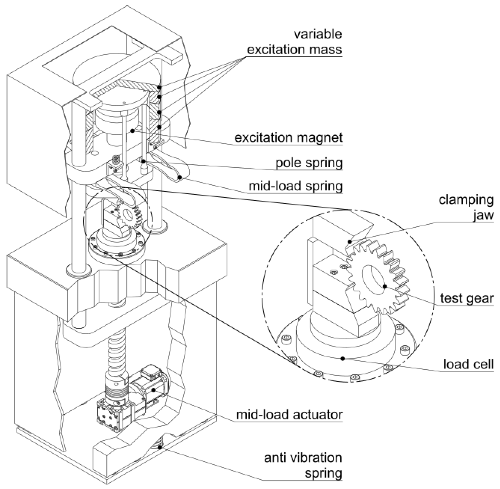
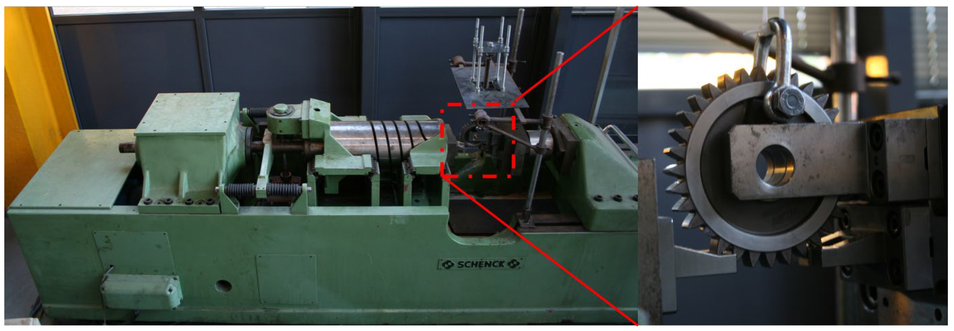
Figure 2 and Figure 3 show two examples of pulsator machines working in symmetrical configurations. All the data discussed here have been obtained with this methodology.
To maintain the specimen in position, pulsator tests must be run with a fixed preload. For instance, the SAE recommendation practice J1619 [32] suggests performing tests at R = 0.1 , while within FVA guideline no. 563 I [25] a load ratio between 0.03 and 0.075 is suggested.

3. The Pulsator to Running Gears Problem

In the previous section, the typical experimental pulsator test rig configurations were presented. The fact that gear teeth are loaded by jaws rather than by rotating gear meshing implies that differences occur between the pulsator test case and the actual application case of MG. Recently, Hong et al. [37], whose testing rig is an asymmetric one, summarized those differences as follows:
1.
Pulsator tests and MG have different loading conditions, as, in the first, a sinusoidal load is applied at a fixed position, while in the latter, the load changes both the magnitude (due to the load sharing between teeth pairs) and the point of application (as the contact point between teeth changes during gear meshing).
2.
The stress ratio R is different as pulsator tests are required to work at R > 0 , while in the MG gear case, the tooth root stress moves to a positive maximum (typically when the contact is at the outer point of a single tooth in contact) to a negative minimum (due to the extension of the compression field from the adjacent tooth, e.g., [4,5,38]), thus at a load ratio R < 0 (e.g., [39]).
3.
The crack initiation location seems to be different. Indeed, certain experimental findings of Winkler et al. [40] and Fuchs et al. [36,41,42,43,44] possibly imply that in the pulsator test case, crack initiation is much more likely to occur at the surface, while in the MG case, a slightly increased risk for subsurface crack initiation can be observed. However, their findings are based on investigations on shot-peened gears made from high-cleanliness steels. Furthermore, a different runout level was considered for pulsator and MG tests. Moreover, considering all the data available [36,40,41,42,43,44], and further results from experimental investigations at FZG that have not been published yet, it can be assumed that there is not a different crack location for common case-hardened gear steels for both compared testing methods (i.e., pulsator and MG). Therefore, the effect of the crack initiation location will not be discussed here.
4.
The statistical behavior of pulsator and MG tests is different. In pulsator tests, the failed teeth are predetermined and are those that are loaded within the pulsator test rig (for each test run, two teeth are in the symmetric configuration); furthermore, not all the gear teeth can be tested. On the other hand, in the MG case, all the gear teeth are loaded during a test run, and the gear failure is the result of the failure of the weakest gear tooth (e.g., [22,29,37,45,46,47]).
Therefore, strength numbers determined by pulsator tests should be elaborated to ensure a reliable estimation for gear design. In 1964, with a slightly different test rig, Seabrook and Dudley [29] already suggested that pulsator experimental strength numbers should be reduced by a factor of 0.77 to account for those differences.
In 1987, Rettig [22] dealt with the problem of the different loading conditions and stress ratio between the test methods. He suggested that, in order to consider the differences in the loading conditions, pulsator test results should be reduced by a factor of 0.9. The validity of Rettig’s coefficient has also been reaffirmed recently by Concli et al. [48,49,50], who adopted high-cycle multiaxial fatigue criteria to estimate the effect of the different stress histories occurring at the tooth root.
In 1999, Rettig’s work [22] laid the groundwork for the estimation procedure reported by Stahl et al. (FVA research project 304) [23]; this approach is discussed in detail in Section 4. This method is completed by the FVA guideline 563 I [25], in which additional information (e.g., the sampling strategy) is provided to the experimenter. According to Stahl et al. [23], pulsator tests should be reduced by a factor of 0.83 for peened and 0.77 for unpeened gears. Those values are completely comparable to what Seabrook and Dudley [29] found.
In 2003 and 2008, Rao and Mc. Pherson [45,46] proposed a different approach. On the one hand, they used allowable stress range diagrams to evaluate the effect of the different load ratios. On the other hand, statistical correlations, similar to the concepts of the return period, were used in order to deal with the statistical problem. A modified staircase procedure was adopted to estimate the experimental procedure. They also observed a difference between the pulsator and MG resembling the one discussed by Seabrook and Dudley [29]. By extension, Rao and Mc. Pherson’s [45,46] findings are also similar to what Stahl et al. [23] calculated.
Between 2021 and 2022, another framework was proposed in [27,28,51]. Two different tools were adopted. Firstly, due to a different load ratio than the one adopted by Rettig [22], high cycle multiaxial fatigue criteria were adopted to deal with the different stress trends [51]. Then, in [27,28], the maximum likelihood method (ML) was adopted to estimate the experimental SN curve. Finally, by means of Statistics of Extremes (SoE), the gear SN curve was estimated. This approach is discussed in detail in Section 5. As will be shown in the following sections, this method yields results similar to that of Stahl et al. [23].
In 2022, Hong et al. [37] also proposed a different estimation procedure. They developed corrective coefficients in order to deal with the first three differences (i.e., the loading condition, stress ratio, and crack initiation location) while statistical relationships (similar to Rao and Mc. Pherson [45,46]) were exploited to develop a fourth coefficient dealing with the statistical differences. They also adopted ML to estimate an experimental curve based on the model of Pascual and Mekker [52]. However, as also discussed by Hong et al. [37], this methodology still needs to be further improved.
It is worth also mentioning two recent works that focus on the topic of experimental pulsator data elaboration. The first is the one of Mao et al. [53], where they developed corrective coefficients to overcome some limitations of the traditional Dixon–Mood method (whose description can be found in [54]). Similarly, to reduce the required specimen numerosity, Alnahlaui and Tenberge [55] proposed a small-sample-size test program based on the linear damage accumulation framework. However, in both works, no further discussions had been made about the estimation of the gear strength starting from pulsator data.
Additional information about the different methodologies and their differences can also be found in [27,37].

4. Method 1: FVA Approach Based on FZG Research

The first estimation method discussed here had been developed at FZG and is defined as a recommended procedure within FVA (Research Association for Drive Technology, in German: Forschungsvereinigung Antriebstechnik e.V.) research according to FVA guideline 563 I [25]. In [25], a practical approach for the evaluation of the tooth root load-carrying capacity, including the gear specimen, pulsator equipment, and test planning, was described. It is based mainly on the work of Stahl et al. (FVA research project 304) [23], where data elaboration is discussed, laying the fundamentals on the analysis of a large number of experimental data performed by FZG. The methodology according to [25] has been developed by examining a symmetric pulsator test configuration for case-hardened gears. Further investigations and detailed statistical analysis of an extended experimental FZG database can be found in Hein et al. [24,26] and Geitner et al. (FVA research project 610 IV) [56]. Refs. [24,56] also reaffirmed the validity of this methodology.
The FVA approach based on FZG research aims to estimate a gear SN curve such as the one described in Figure 4. Here, different considerations are made regarding the limited-life and long-life regions. On the one hand, for each load level, the first region presents a different lognormal deviation of the failure load cycle number. In other words, the dependency of the variance with respect to the load level is considered (see also Figure 6). On the other hand, the long-life region is described by an endurance limit, whose dispersion is in the load/stress direction. For both the experimental and gear SN curves, these two regions are estimated separately using two different calculation procedures.
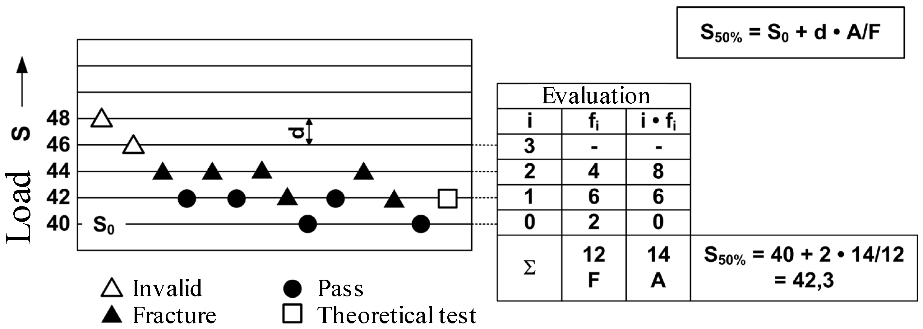
According to this method, the experimental endurance limit is estimated according to Hück [57]. It is assumed that the experimental endurance limit follows a normal distribution. In the case of reduced sample size (n < 10), this method suggests estimating the experimental endurance limit by adopting the modified probit method as defined by Hösel and Joachim [58]. Figure 5 shows an example of the application of the Hück [57] approach, displaying a staircase test sequence together with an additional theoretical test run. The experimental endurance limit σ F 0 , 50 % is defined starting from the determination of the number of tests f i on load level i , leading to the sums F and A .
According to Hück [57], σ F 0 , 50 % is defined as:
σ F 0 , 50 % = σ F 0 , i = 0 + d · i · f i f i = σ F 0 , i = 0 + d · A F
Once the σ F 0 , 50 % has been estimated, the gear endurance limit σ F 0 , 1 % , M G (under the MG loading condition) is calculated by means of corrective coefficients [23]:
σ F 0 , 1 % , M G = f 1 % F D · f P M G · σ F 0 , 50 % , P
where f 1 % F D is equal to 0.92 for peened gears and 0.86 for unpeened gears according to Stahl [23]. An additional coefficient f P M G equal to 0.9, defined by Rettig [22], is adopted to take into account the load differences. f P M G was not applied in this paper; that is, σ F 0 , 50 % must be reduced by 0.77 or 0.83 to estimate σ F 0 , 1 % , M G .
Within method 1, the limited-life region is estimated by calculating, for each load level, the 50% experimental lifetime N 50 % by assuming a log-normal distribution of the failure load cycle numbers [23]. This is performed using a log-normal probability grid, with the definition of the single failure probability for each data point based on the order approach defined by Rossow [59]. On the other hand, a more simplified approach is to calculate N 50 % from the lifetime of the n individual tests according to Equation (3) [25]:
log N 50 % = 1 n i = 1 n log N i
That is, calculating the average lifetime.
Once the 50% curve has been estimated, the 1% gear failure probability lifetime N 1 % is calculated for each load level as:
N 1 % = 10 ( log N 50 % 2.33 · s l o g
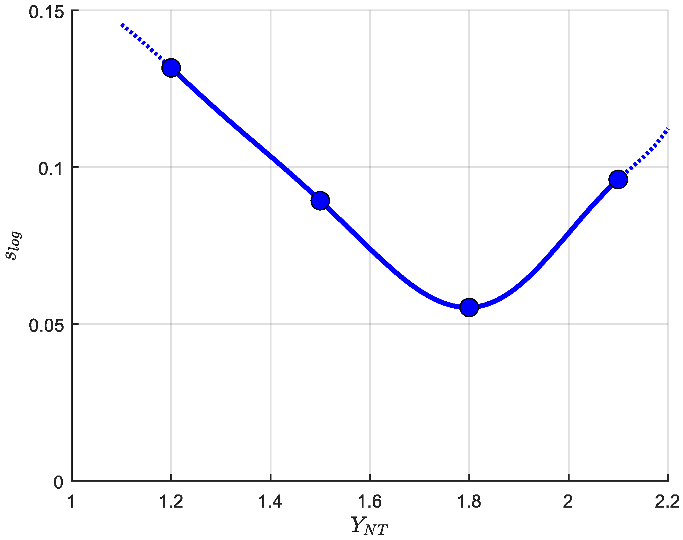
where s l o g is the typical logarithmic standard deviation, the trend of which is shown in Figure 6. Then, both the 50% experimental and the 1% gear curve are calculated by fitting a line through the estimated log N 50 % and log N 1 % .
According to this method, the standardized calculation method as per ISO 6336-3 [6] can still be applied. Therefore, the life factor Y N T is used to multiply σ F 0 , 1 % , M G . The choice between a horizontal endurance line and the presence of the secondary slope for a number of load cycles > 3 million depends on the experience and the criticality within the field of application.
The FVA guideline 563 I [25] also describes the sampling strategy adopted (i.e., allocation and numerosity). According to this guideline, six different load levels are to be selected (if possible), two of which should be in the limited-life range. The load levels for the determination of the endurance limit must be equally distanced. Between 28 and 38 data points are suggested for a high numerosity experimental campaign. However, the standard allocation is between 20 to 24 test runs. The FVA guideline 563 I [25] also suggests that half of the specimens should be located in the endurance limit region while the remaining should be distributed among the load levels, aiming to have at least two load levels with a higher numerosity. Experimental campaigns with low numerosity are still possible, especially when the focus is primarily on the endurance limit. The runout level (i.e., the limiting load cycle number) is set to 6 million load cycles in pulsator tests.
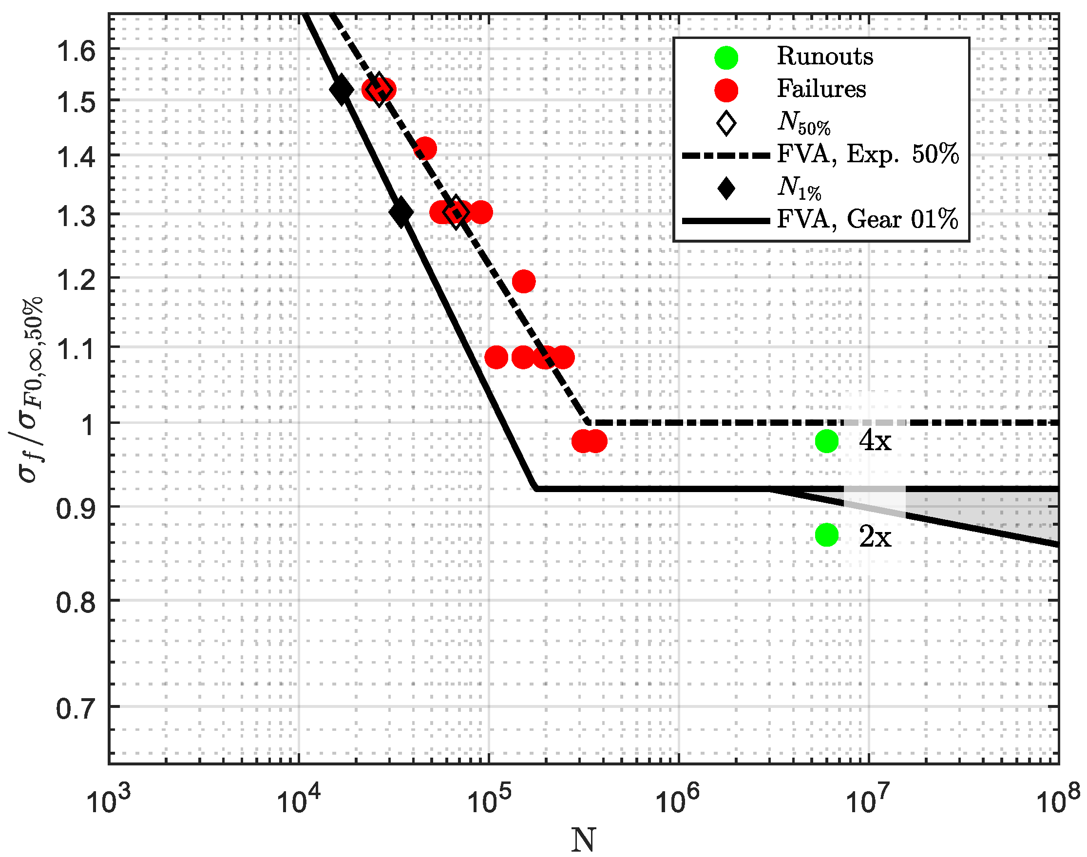
An example of the application of this procedure is shown in Figure 7, where the dotted curve represents the 50% experimental SN curve while the continuous curve is the 1% gear curve. Here it is possible to observe the effect of the hypothesis of a not-constant deviation for the limited life. Indeed, the slopes associated with the limited life slightly vary. Similar to Figure 1, a shaded area has been included to represent the possible choices of Y N T . The term “Exp” refers to the 50% curve estimated considering the experimental point while the term “Gear” refers to the gear SN curve (at 1% failure probability).

5. Method 2: Maximum Likelihood and Statistic of Extremes (ML&SoE)

Differently from the estimation approach presented in the previous section, in [27,28], a gear SN curve estimation approach was proposed based on two different tools: The ML method for the estimation of the experimental SN curve and SoE for its translation to the gear SN curve. Here, a two-slope curve formulation is adopted to describe the SN curve according to Spindel and Haibach [60]. According to this approach, the experimental SN curve can be described as:
log N = log N e + 1 2 k 1 + k 2 log σ log σ e + + 1 2 k 1 k 2 log σ log σ e
where N e and σ e are the coordinate of the knee, and k 1 is the slope associated with the limited-life region and k 2 for the long-life region.
This model also features a constant standard deviation in the log σ direction s log σ F 0 that, due to the first-order approximation [61], results in two different standard deviations in the log N direction s 1 , log N and s 2 , log N [60]. This model is also called the “bilinear uniform scatter band” (e.g., [62]). Data points are considered log-normally distributed, and differently from method 1 (see Section 4), all the points are considered part of a unique dataset. Therefore, here the distinction between limited-life and long-life regions depends only on the estimation outcome.
In order to estimate the teeth SN curve according to Equation (5), it is necessary to adopt the ML method due to the presence of survived specimens (i.e., specimens whose failure has not been observed) [61,63,64]. By considering the symmetric pulsator test configuration, depending on how the experimental data are considered, two different kinds of data can be obtained:
1.
If the experimental points are considered as they are, that is, if the fact that the symmetric test configuration works on two teeth is not considered, the only observed surviving specimen is the one that reaches the runout level. The elaboration performed with such considerations is called “STBF” as they are the experimental points obtained directly from the pulsator/STBF testing machine.
2.
If the fact that the symmetric test configuration works on two teeth is considered, it must be considered that the experimental point is not composed only of failed and surviving specimens but by the compresence of both. This can be easily understood by looking at the experimental points. On the one hand, if one of the two teeth fails (i.e., a failure according to the STBF consideration), the other has survived. That is, a failure occurring within the test is both an observed value (i.e., the failed tooth) and randomly right-censored data (i.e., the survived tooth). On the other hand, if the runout level is reached (i.e., a runout according to the STBF consideration), both tested teeth have reached the runout level. Therefore, different statistical considerations must be taken into account in the 2T case. The elaboration performed with such considerations will be called “2T” as two teeth are taken into consideration.
Details about the ML estimation of Equation (5) curve (together with s log σ F 0 ) are reported in Appendix A. Once the initial curve parameters have been estimated, it is necessary to estimate the curve describing the gear. This is achieved by considering the hypothesis that in the case of tooth root bending fatigue, the gear fails when its weakest tooth breaks [22,29,37,45,46,47]. Therefore, SoE is used to elaborate the teeth Cumulative Distribution Function (CDF) to estimate the gear CDF. Through a mathematical passage, it allows for the estimation of the CDF describing the lowest value that can be observed by sampling n times from the same population. On the one hand, the term “lowest value that can be observed” is the weakest tooth (that describes the gear). On the other hand, the “same population” is represented by tested teeth and is described by a log-normal distribution whose mean is defined according to Equation (5) and standard deviation σ log σ F 0 .
When the STBF curve is studied, it is necessary to consider that this curve is based on a teeth pair, of which we observe the lifetime of the weakest one. By considering the gear as a system of z/2 teeth pair, it is possible to estimate the gear CDF F g e a r as:
F g e a r = 1 1 F S T B F z / 2
Similarly, when the 2T curve is studied, F g e a r is defined as:
F g e a r = 1 1 F 2 T z
Different curves at different reliability levels can be obtained by calculating the corresponding percentile for several load stages.
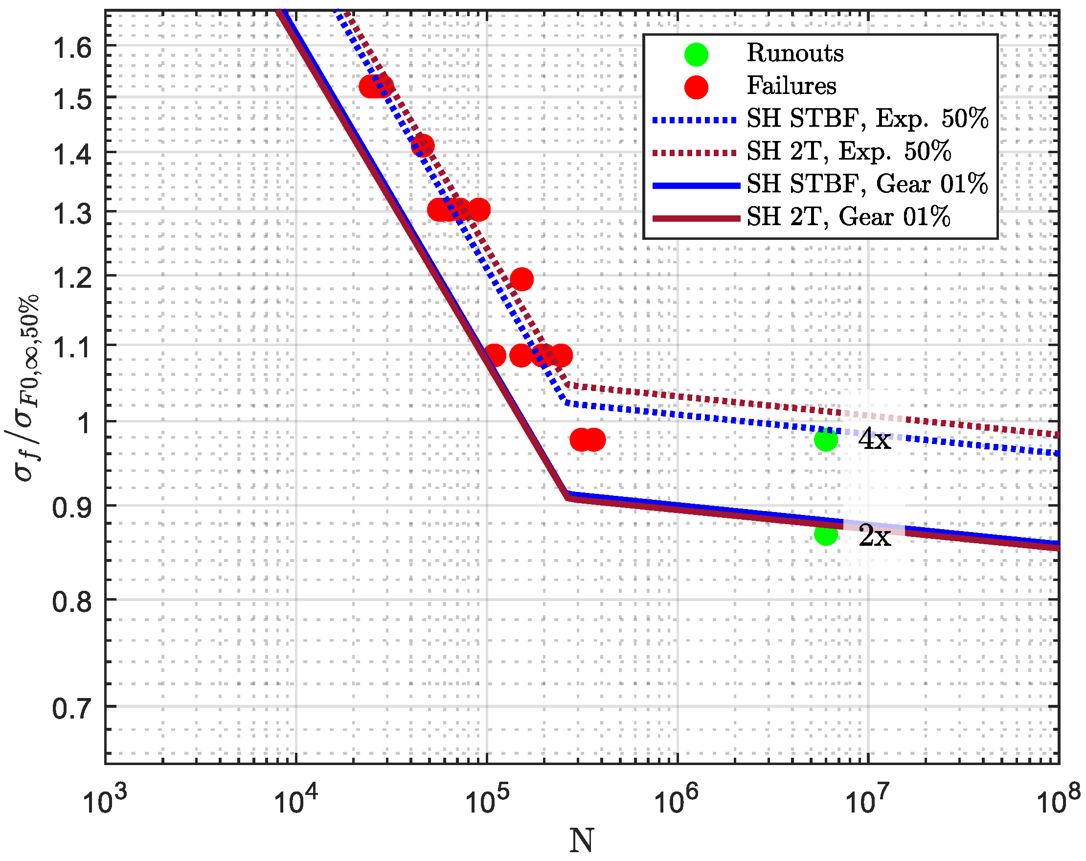
An example of the application of this procedure is shown in Figure 8; here, the experimental points are the same as in Figure 7. The dotted curve represents the curve that estimates the SN curve of the exemplary campaign according to the STBF and 2T approximation, while the continuous lines are the gear SN curves, estimated according to Equation (6) or Equation (7). On the one hand, the comparison between the STBF and 2T curves allows us to understand the role of the 2T consideration. The 2T curve is slightly above the STBF one. On the other hand, focusing on the gear SN curves, it is possible to notice that both estimation methods lead to (almost) completely identical curves.

6. Adopted Database

The analysis presented in the following sections was carried out by taking advantage of the case-hardened gear database present at FZG, combined with the one presented by the gear research group at POLIMI. That is, all the data have been obtained by the authors’ research groups.
FZG points have been partially described and analyzed by Hein et al. [24] considering the data contained in [40,65]. Focusing on the effects of materials and heat treatment properties, FZG data have been also analyzed in [56]. All associated FZG test campaigns described in [24] were performed after 2002 and were not available at the time of the work performed by Stahl et al. (FVA research project 304) [23]. More precisely, most of them have been performed in the last decade. POLIMI data points have been described in [27,28,66,67]. POLIMI test campaigns have been performed in the last two decades. Table 1 summarizes the database references in chronological order.
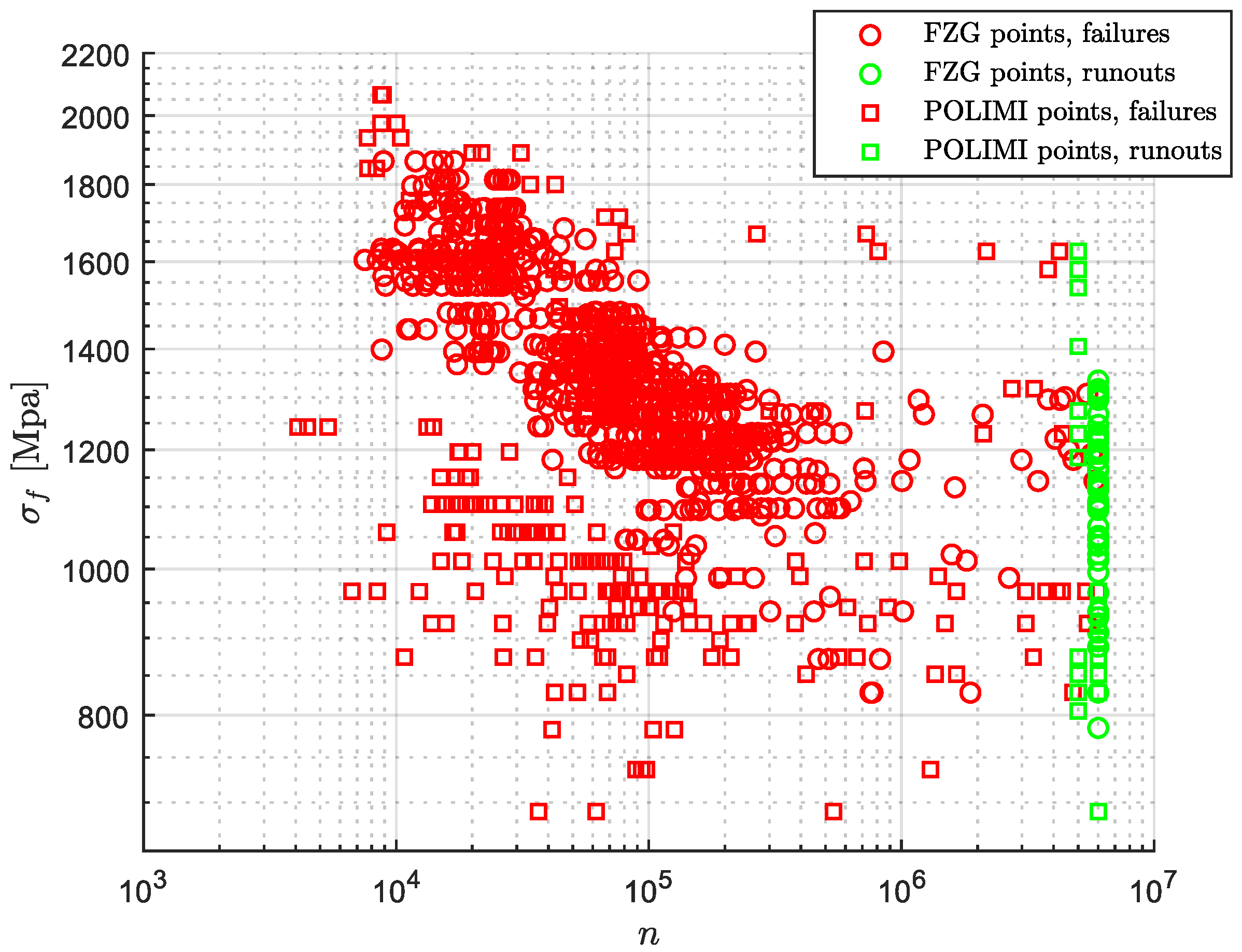
Consequently, the analyzed test data represents up-to-date properties of commonly used case-hardened steels for gears. The database also includes tests supported by industrial sponsoring. Due to the confidentiality and comparability of the test campaigns, the exemplary test data are illustrated as anonymized and normalized. Furthermore, as will be subsequently mentioned in the paper, the test methodologies comparison has been performed on several further cases, which are not shown in this paper for the sake of simplicity. Figure 9 shows the database adopted here. It is composed of 1643 data points, divided into 76 experimental campaigns.

7. Evaluation Study: Comparison between the Two Models

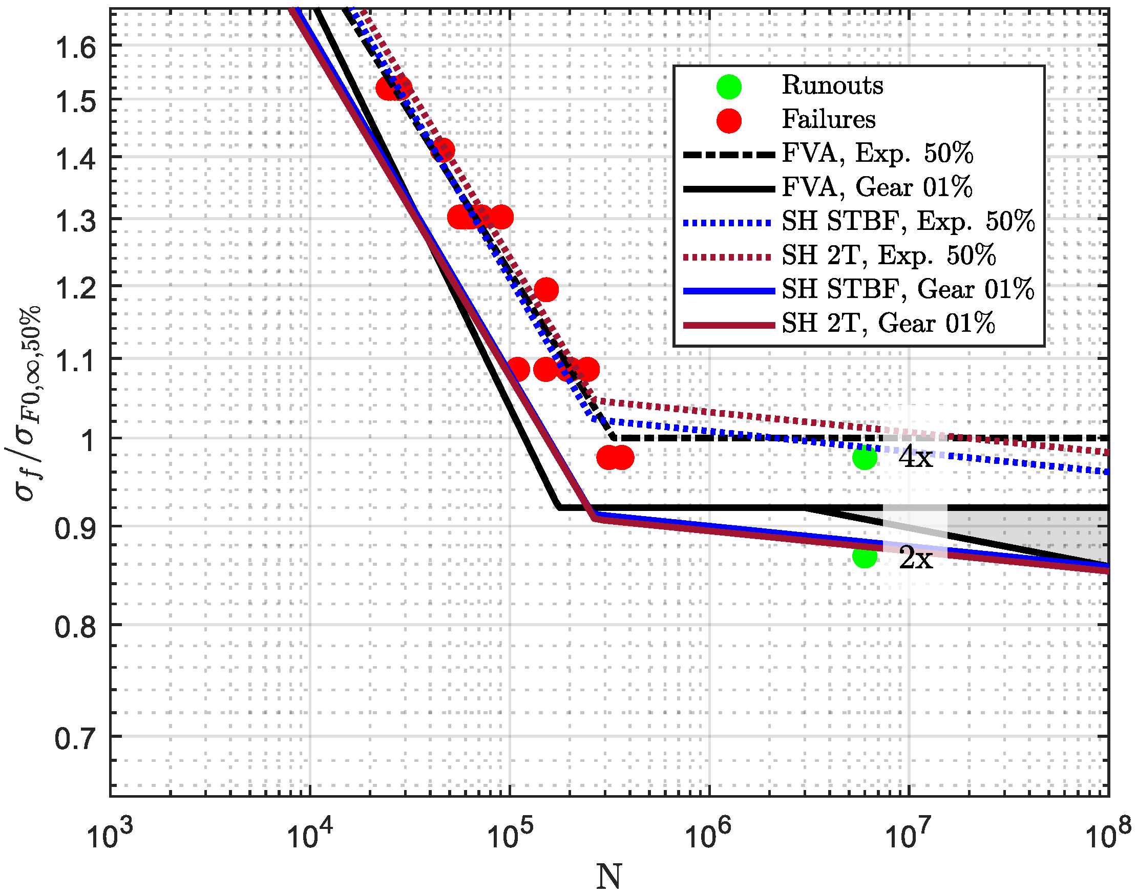
The simplest comparison between method 1 and method 2 is the direct comparison between the curves estimated with the two different approaches. Figure 10, Figure 11, Figure 12, Figure 13 and Figure 14 show the outcomes of these two elaboration methods for five different pulsator test experimental campaigns. Several cases have been studied, obtaining similar results. For the sake of simplicity, only five of them are shown. For all the experimental campaigns, the solutions of method 2 have been verified by adopting the Likelihood Profile (LP) and Likelihood Ratio (LR). Experimental points shown in Figure 10 to Figure 13 were taken from the FZG database [24] while those in Figure 14 were obtained at POLIMI [27,28]. The SN curve comparison has not been extended to other Section 3 methodologies because they require specific data that are not available.
By looking at the gear SN curves shown in Figure 10, Figure 11, Figure 12, Figure 13 and Figure 14, it seems that there is no relevant difference between the two estimation techniques as the estimated curves are close to each other, especially if Y N T according to ISO 6336-3 [6] is selected on the conservative side in the long-life range. The good agreement between the models allows us to re-affirm the validity of the two models: Despite the usage of completely different statistical tools, the final gear curves are different but, most importantly, they are coherent with each other.
The first difference between the two estimation methods is the different positions of the fatigue knee. Especially for the Exp. curves, method 2 always estimates the knee above the one estimated by method 1. This different position is related to the different estimations of the complete SN curve. On the one hand, according to method 1, the fatigue knee is estimated as the intersection of the line describing the limited-life and the long-life regions. On the other hand, according to method 2, the fatigue knee location depends on the two estimated CDF parameters ( N e and σ e ) and the CDF elaboration. However, neither method 1 nor method 2 present a smooth passage between the two regions. This aspect is taken into account within more complex SN curve estimation methods (e.g., [68,69,70,71,72,73]). Their application within the case of pulsator test elaboration is the subject of current research.
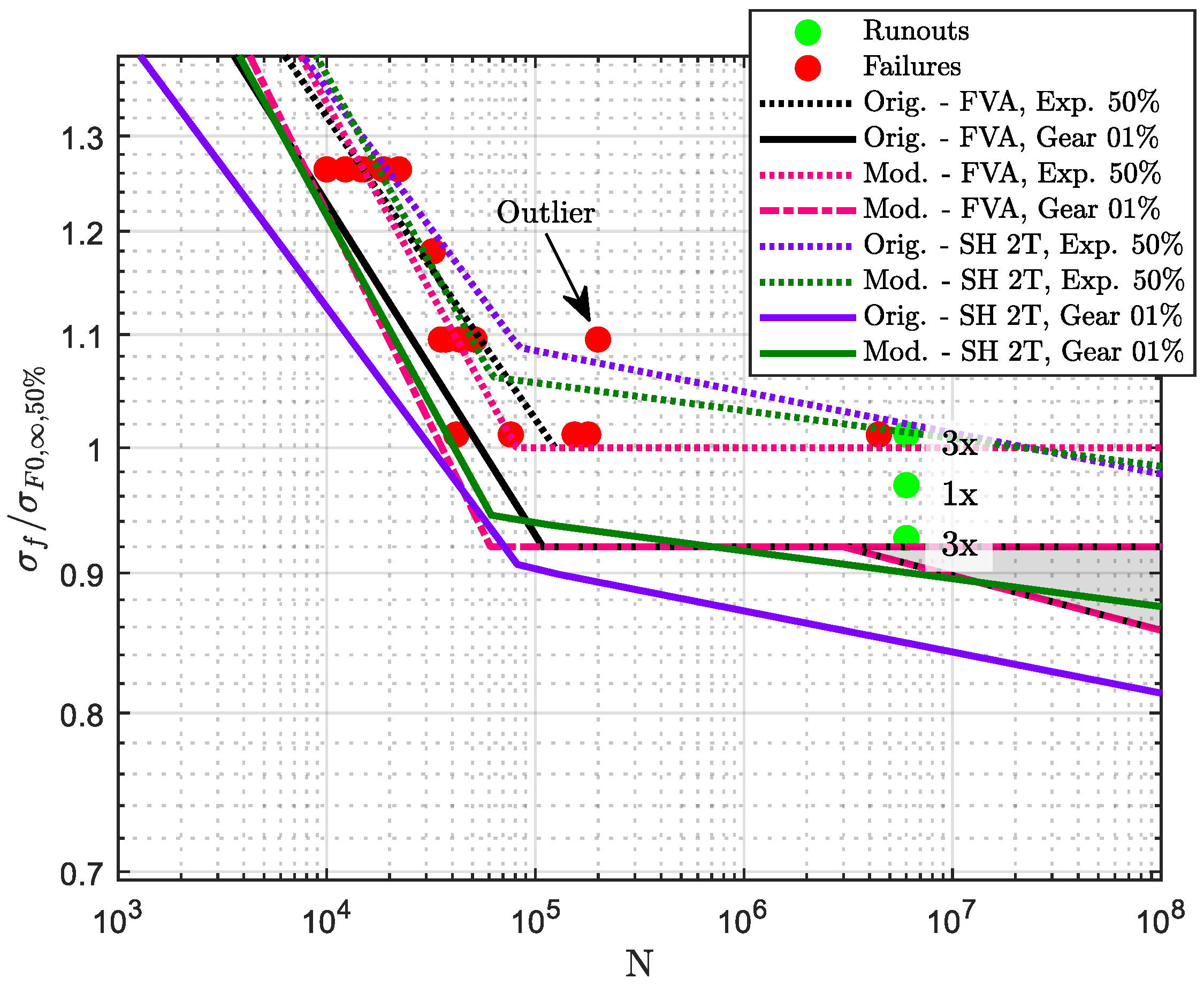
The main difference between the two estimation methods is the model sensitivity concerning the presence of outliers, and method 2 results in being more sensitive than method 1. This is depicted in Figure 13, where one experimental point (i.e., the one indicated by the arrow) can be considered an outlier as it has a lifetime almost 5 times higher than the one of the other experimental runs obtained at the same load level. This outlier has been defined by a graphical analysis of the test data and adopted here as an example.
On the one hand, concerning method 1, the only effect the outlier has is that, at such a load level, N 50 % (i.e., Equation (3)) changes, with consequences on the estimated N 1 % (i.e., Equation (4)); the lines describing the experimental and gear-limited life vary accordingly (see the relatively slight difference between the pink and the black line). As limited-life and long-life regions are estimated differently, this outlier does not affect the latter. Furthermore, as method 1 moves the estimated curves according to pre-defined coefficients (based on the typical scatter), the presence of an outlier has a minor effect as it affects only the estimated means. Indeed, both the original (i.e., the black one) and modified curves (i.e., the pink one) remain close to each other.
On the other hand, in method 2, it is possible to note how the identification of outliers is a crucial aspect. The two estimated curves are significantly different in both the limited-life and long-life regions, especially in the latter. Here, if the outlier, whose lifetime is the highest at the load level, is removed, the new gear SN curve indicates a higher resistance. This counterintuitive behavior is related to the estimation of s log σ F 0 . As a unique standard deviation is estimated by the model (i.e., s log σ F 0 ), the presence of outliers implies an overestimation of s log σ F 0 . Such overestimation leads to a higher variance associated with the long-life region, with a detrimental effect on the gear SN curve. This aspect turns out to be the most crucial one. Furthermore, it is also possible to note how, as the model considers all the experimental points as a unique dataset, high load level points influence the long-life region (and vice versa).
Nevertheless, once the outlier has been removed, both methods 1 and method 2 give, once again, similar results.

8. Extended Investigations on Method 2

As mentioned in Section 4, the validity of method 1 had been reaffirmed in recent works (i.e., [24,56]). Both in [27] and here, the initial validation of method 2 was performed by comparing—partially—the outcome of the two models discussed here.
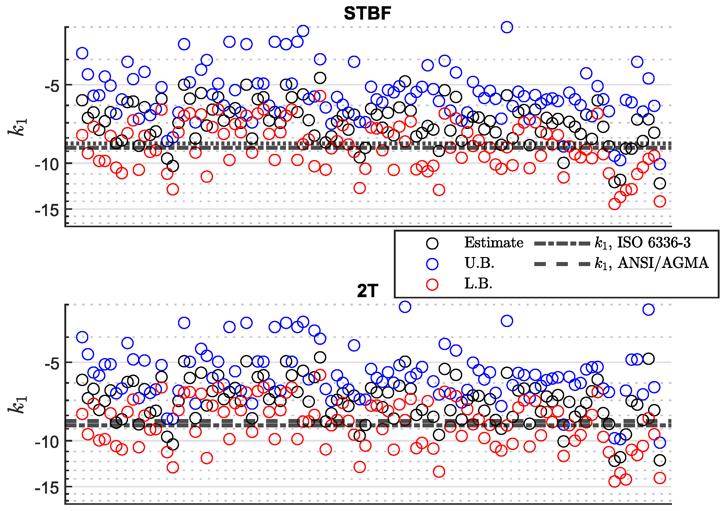
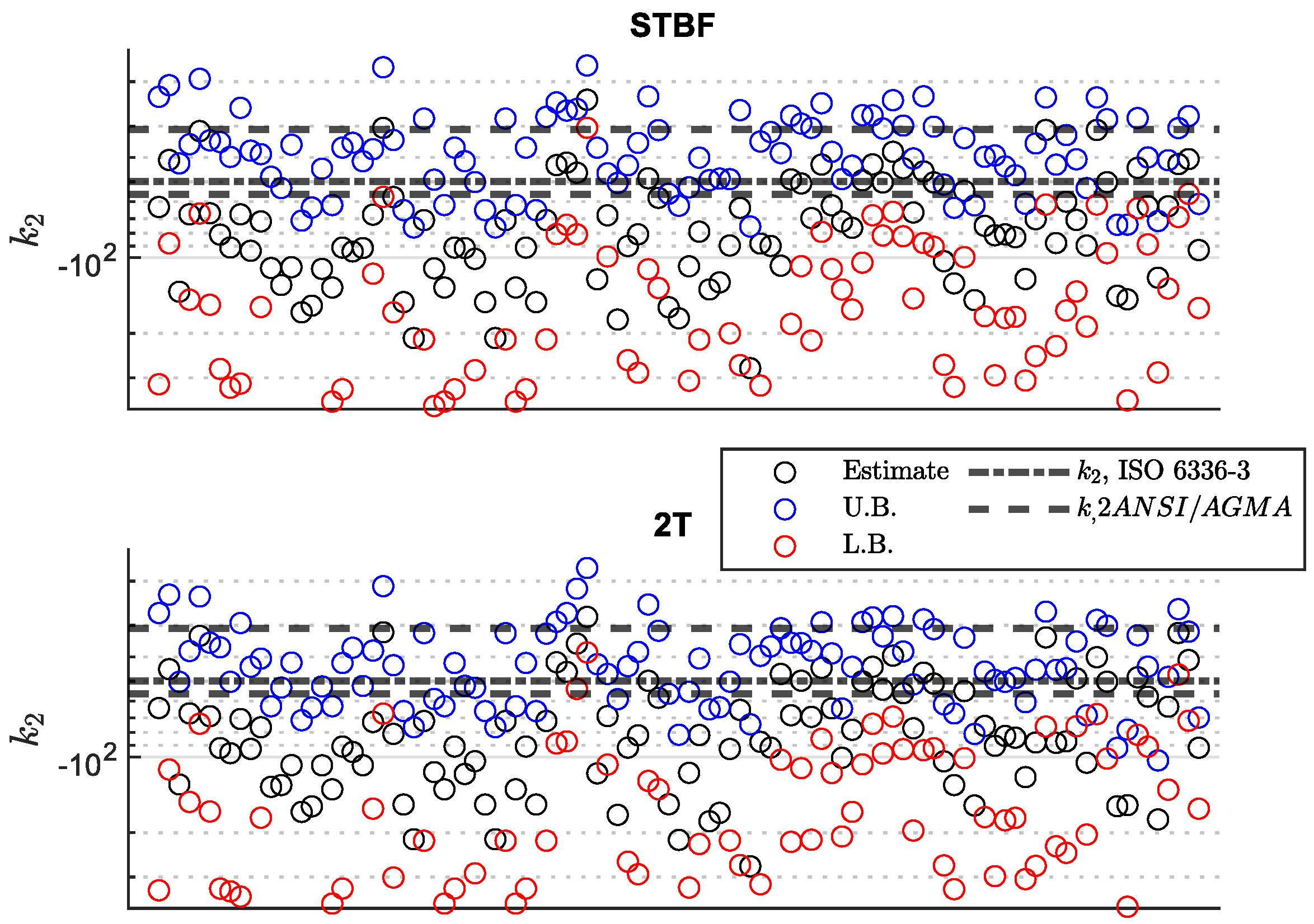
Further validation of method 2 can also be performed by comparing the outcome of the model parameters (together with their confidence interval) with typical gear data. Such validation is performed by examining the confidence intervals of k 1 and k 2 . Confidence intervals are then compared with the typical values, which are the slopes of the limited-life and the long-life region for case-hardened materials according to ISO 6336-3 [6] and ANSI-AGMA 2001 [7].
The parameters N e and σ e were not considered. On the one hand, it is clear that in the database of Figure 9, the fatigue knee is not located at 3 million cycles (also see examples from Figure 10, Figure 11, Figure 12, Figure 13 and Figure 14). On the other hand, discussion about σ e cannot be conducted for two reasons. Firstly, different from ISO σ F   l i m (i.e., the nominal bending stress number), σ e cannot be seen as either an endurance limit or as a fatigue limit. Indeed, σ e is just a parameter of Equation (5); therefore, it lacks all the statistical properties of an endurance (or fatigue) limit. Secondly, if one supposes that σ e is equivalent to σ F   l i m (or to ANSI-AGMA s a t ), the comparison will become a comparison between the estimated material endurance limits and their standardized equivalent (which, in any case, is not the aim of this article).
The methodology adopted here takes inspiration from previous works. One example is the work of Beretta et al. [74] in which they performed a Monte-Carlo simulation of a fatigue database composed of 188 test data in order to investigate how to properly estimate a SN curve. Then, several testing conditions were simulated and the convergency of the parameter confidence interval was compared, aiming to define the best sampling strategy. A similar procedure was adopted by Loren and Lundtröm [75,76], where 100 staircases were virtually simulated to validate their models by comparing the estimates. Similar methodologies for the evaluation of the behavior of stress-lifetime models can also be found in [53,55,77,78].
Here, to increase the number of available experimental campaigns, as well as the numerosity of experimental campaigns with a high number of experimental points, some test series about similar gears made with comparable materials and treatments were combined. Twenty-seven new experimental campaigns were defined accordingly. Details about the confidence interval calculation according to LR are shown in Appendix B.
Figure 15 and Figure 16 show a comparison between the estimated slopes (and their two-sided 95% confidence intervals) with their equivalent according to gear standards for both STBF and 2T. For most cases, the standardized values lie within the confidence interval. Based on this analysis, it is not possible to state that the estimated slopes are statistically different from the ones suggested by the standards. This behavior is particularly true for k 1 and k 2 according to ISO 6336-3 [6] and for k 1 and the highest (absolute) value k 2 according to ANSI-AGMA 2001 [7]. Therefore, it can be concluded that the parameters estimated by method 2 are not different from the typical ones of case-hardened gears.
As already mentioned, the FVA guideline 563 I [25] also provides indications about the allocation and numerosity of specimens. Those values have been defined within the context of data elaboration according to method 1. An indication of the number of experimental points required by model 2 can be obtained by taking inspiration from Beretta et al. [74].
Here, the Figure 9 database is used to evaluate the convergency of the parameter’s confidence interval. Only the parameter s log σ F 0 is shown here. The rationale for this is that the variance is the crucial parameter for calculating the different percentiles. Furthermore, the other parameters all show an earlier convergency. As the database is composed of several materials, the comparison is performed by observing the normalized parameter.
Figure 17 shows the convergency of s ˜ log σ F 0 / s ^ log σ F 0 , that is, the convergency of the LR-based confidence interval s ˜ log σ F 0 (bilateral at 95%) normalized over the estimated one (i.e., s ^ log σ F 0 ). Both STBF and 2T cases are shown. In total, 103 experimental campaigns have been evaluated. Looking at the trend, after approximately 25–30 experimental points, there is no significant reduction in the confidence interval. Thus, 25–30 experimental points are the minimum number of points required for proper parameter estimation. In other words, 25–30 experimental points are required for a proper gear SN curve estimation if model 2 is adopted (30 to be on the conservative side).

9. Conclusions

Pulsator/STBF test is a test method employed in the estimation of gear tooth root load-carrying capacity with respect to the tooth root fatigue fracture phenomena. It is widely adopted because it is a cost-efficient method that considers a representative test specimen. Typical applications of pulsator tests are investigating the effects of material heat and surface treatments in gears. However, the pulsator test procedure presents several differences with respect to the real-world case where gears are meshing under load. Therefore, pulsator test results must be elaborated before using them to design a gear pair. Several methodologies have been developed over the years. Considering that all of them have been developed for different test configurations, good agreement has been found. That is, all of them suggest that, in the long-life region, pulsator test results should be reduced by a factor of approximately 0.77 0.83 .
Among all the methodologies, two of them have been developed by examining a symmetric (double teeth) pulsator test configuration. These two methodologies are discussed here in detail. The first (method 1: FVA, based on FZG research) elaborates pulsator test data based on typical scattering values obtained from a previous case-hardened gear test, that is, it adopts pre-determined coefficients. It must be noted that this methodology covers the whole testing procedure as additional information is also provided (e.g., gear specimen, testing machine). Most importantly, it also provides the experimenter with indications about the test planning. From a statistical and mathematical point of view, this methodology can be considered the simplest one. The latter (method 2: ML&SoE) adopts ML to estimate the experimental curve; then it estimates the gear SN curve by means of SoE. Different from the previous one, this methodology relies only on the observed data within the analyzed test series. However, no discussions about test planning have been performed so far for method 2, especially concerning specimen numerosity.
The two approaches discussed in this paper have been defined, independently and at different times, by all the authors of the paper. Both methodologies are described here in detail. In this way, the designer who wants to undertake the task of gear testing can find indications about the elaboration of pulsator test data.
The comparison of the methodologies has been performed on the basis of an actual database composed of 1643 symmetric pulsator test results obtained during 76 different experimental campaigns on case-hardened gears. The comparison was performed by directly examining the final gear SN curve. It has been found that both methods yield completely comparable results. The good agreement between the corresponding outcomes allows us to reaffirm the validity of the two models. However, as it does not rely on previously defined data, method 2 tends to be more sensitive to the presence of outliers. Several cases have been studied; for the sake of simplicity, only a few of them are reported in this paper.
As mentioned in Section 4, the validity of method 1 has been reaffirmed recently. Nevertheless, for method 2, both here and in previous works, the validation of method 2 has been performed only by comparing the outcomes of method 1 and method 2. Further validation of method 2 has been conducted here due to the availability of the case-hardened gear database. Parameter confidence intervals have been compared with typical gear data, finding good agreement between the model outcomes and their equivalents presented by the standards. Furthermore, the minimum number of points required for the application of the method has been calculated. This has been calculated as 30 to be on the conservative side.

Author Contributions

Conceptualization, L.B. and M.G.; methodology, L.B. and M.G.; software, L.B.; supervision, T.T., C.G. and K.S.; writing, L.B. and M.G. All authors have read and agreed to the published version of the manuscript.

Funding

This research received no direct external funding. However, the experimental database used includes results from several research projects over previous decades funded by different associations.

Institutional Review Board Statement

Not applicable.

Informed Consent Statement

Not applicable.

Data Availability Statement

Data are available normalized upon reasonable request.

Conflicts of Interest

The authors declare no conflict of interest.

Acronym

The following acronyms are used:
CDFCumulative Distribution Function
MLMaximum Likelihood
MGMeshing Gear
LRLikelihood Ratio
PFProfile Likelihood
PDFProbability Density Function
STBFSingle Tooth/Teeth Bending Fatigue
SoEStatistics of Extremes

Nomenclature

A Parameter of Hück method
d Stress/load step, mainly considered in Hück method
γ 1 Generic model parameter
γ ^ 1 Estimated parameter
γ 1 ¯ Constrained parameter
γ ˜ 1 Confidence interval of the estimated parameter
F Parameter of Hück method
F g e a r Gear CDF
F S T B F STBF CDF
F 2 T 2T CDF
f i Number of tests on the i t h load level, Hück’s method
f 1 % F D Conversion factor acc. to Stahl for 50 % to 1 % failure probability
f P M G Corrective coefficient acc. to Rettig
k 1 Limited life slope
k 2 Long life slope
L Likelihood
l Log-likelihood
N 50 % 50% experimental lifetime
N 1 % 1% gear failure probability lifetime
N e Spindel-Haibach model coordinate (together with σ e )
s Standard deviation
s l o g Logarithmic standard deviation
s log σ F 0 Spindel-Haibach standard deviation in the log S direction
s 1 , log N Spindel-Haibach standard deviation in the log n direction, limited life region
s 2 , log N Spindel-Haibach standard deviation in the log n direction, long life region
σ Stress
σ e Spindel-Haibach model coordinate (together with N e )
σ F 0 , 50 % Experimental endurance limit for 50 % failure probability
σ F 0 , 1 % , M G Gear endurance limit for 1 % failure probability
Y N Life factor acc. to ANSI/AGMA 2001
Y N T Life factor acc. to ISO 6336-3

Appendix A. Maximum Likelihood Estimation of the Experimental Tooth Root Fatigue Fracture SN Curve

ML is a parameter estimation technique based on finding distribution parameters that are most likely to describe the collected data. Mathematically, those estimated parameters are the ones that maximize the likelihood. Such an estimation technique is typically adopted to estimate the stress–life relationship of components (e.g., fatigue specimens, insulations, etc.). More complete details about this estimation method can be found in [61,63,64,79].
One of the greatest advantages of ML is its capability to deal with different kinds of data. Indeed, within the same statistical framework, it is possible to take into account, together with its statistical meaning, failures (i.e., observed data), survivals (i.e., right-censored data), failures occurring within different inspections intervals (i.e., interval-censored data), and failures occurring before the first inspection interval (left-censored data). In the case discussed here, only observed data and right censored data are present. For the Spindel–Haibach model (i.e., Equation (8)), the likelihood L can be described as:
L = i = 1 n f x i ; μ , σ δ i i = 1 n 1 F x i ; μ , σ 1 δ i
where f x i ; μ , σ and F x i ; μ , σ are the PDF/CDF describing the phenomena and μ and σ are the parameters of the normal distribution (i.e., mean and standard deviation). δ i is equal to 1 in the case of observed data and 0 in the case of right-censored data. i = 1 n f x i ; μ , σ δ i is the term used to refer to observed data and i = 1 n 1 F x i ; μ , σ 1 δ i is the one referring to right-censored data. Here, μ and σ are defined according to Section 5.
However, in order to facilitate the parameter estimation procedure, it is typical to work on the log-likelihood l (i.e., the logarithm of L ), as the same properties apply:
l = ln L = i = 1 n δ i ln f x i + i = 1 n 1 δ i ln 1 F x i
Considering a model with p parameters γ 1 , γ 2 , , γ p , the estimated parameters γ ^ 1 ,   γ ^ 2 , ,   γ ^ n are those that maximize the log-likelihood:
l ^ = l γ ^ 1 ,   γ ^ 2 , ,   γ ^ n = max γ 1 , γ 2 , , γ p l γ 1 , γ 2 , , γ p
where l ^ is the maximum log-likelihood.
From a practical point of view, as typical calculation software does not present maximization algorithms, γ 1 ^ , γ 2 ^ , , γ p ^ are estimated by minimizing l .

Appendix B. Profile Likelihood and Likelihood Ratio Profile
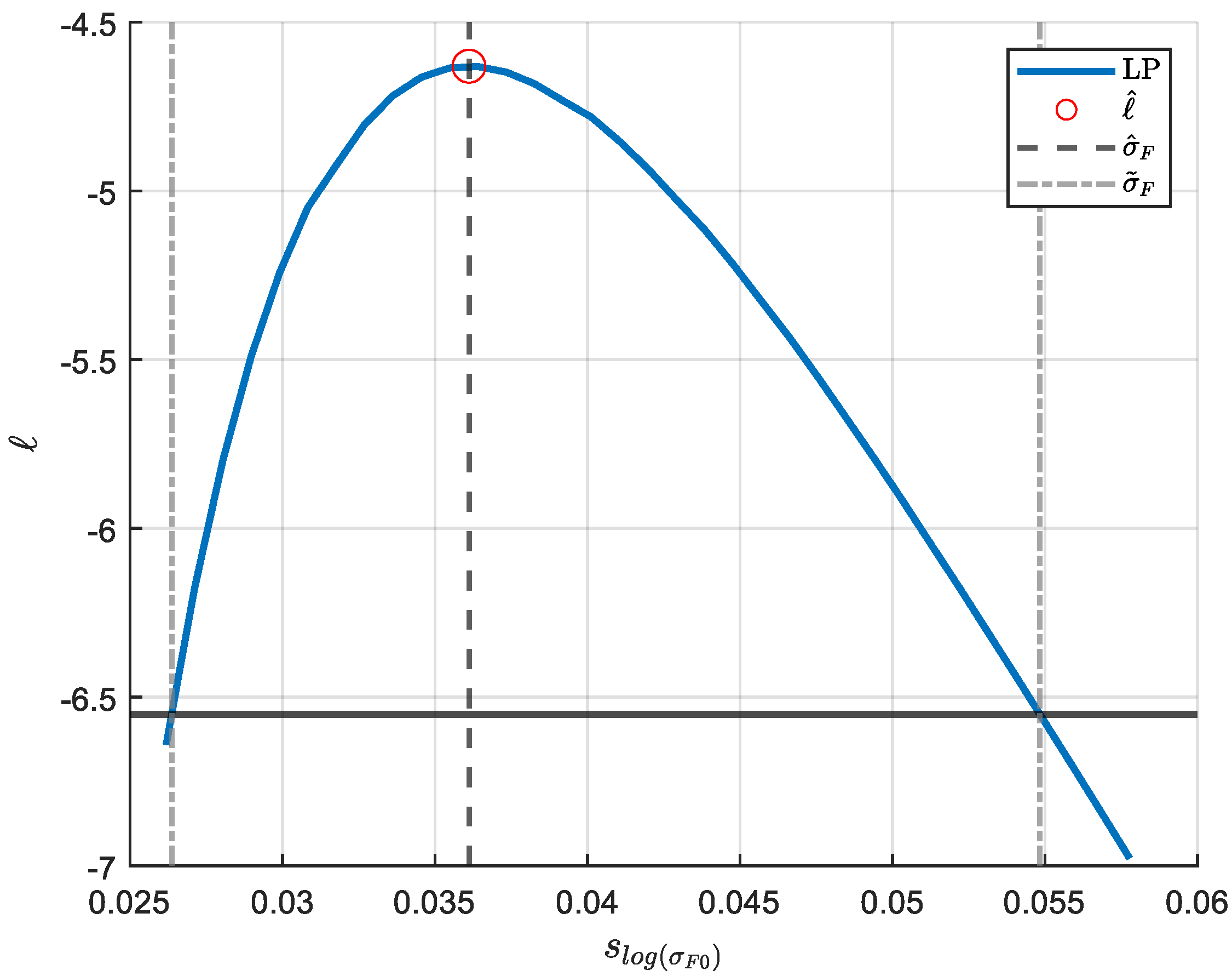
Profile Likelihood (PF) refers to the possibility of expressing how L (or l ) depends on the parameters [61,63,64,80,81]. PF is formulated by constraining one (or more) parameter/s and calculating the new maximum likelihood. In other words, LR describes the trend of the constrained maximum likelihood in a certain range of the constrained parameter. However, as L cannot always be easily computed, it is typical to describe PF using l rather than L . If γ 1 is constrained to be equal to γ ¯ 1 , the constrained maximum log-likelihood for γ 1 ¯ can be defined as:
l γ ¯ 1 = max γ 2 , , γ p l γ 1 = γ ¯ 1 , γ 2 , , γ p
An example of PF is shown in Figure A1, where the PF has been calculated for several values of s log σ F 0 .
Figure A1. Example of LP and LR for s log σ F 0 .
Applsci 13 01546 g0a1
The usage of PF allows for the description of the confidence interval of the parameter in its natural range [61,63,64] via the usage of the Likelihood Ratio (LR). It is possible to demonstrate that the ratio between l ^ and l γ ¯ 1 can be related to a χ 2 distribution with one degree of freedom [82]:
2 ln R γ 1 = 2 ln L γ ¯ 1 L ^ = 2 l ^ l γ ¯ 1 ~ χ 1 2
According to Equation (12), it is possible to express the confidence interval of the parameter γ 1 with a 1 α confidence level (i.e., γ ˜ 1 ) by finding the value of γ 1 ¯ that satisfies Equation (13) [61,63,64].
l γ ¯ 1 = l ^ 1 2 χ 1 α , 1 2
Figure A1 also shows the confidence interval s ˜ log σ F 0 evaluated according to Equation (13).
It is worth mentioning another utility of the LR framework. Indeed, most minimization tools such as (e.g., MatLab’s fminsearch) require an estimation of the solution as an input parameter. By calculating the LP, several guess solutions are provided, thus allowing one to properly investigate, whereas the solver has calculated a proper solution.

References

  1. Aktiengesellschaft, M. Maag Gear-Book: Calculation and Manufacture of Gears and Gear Drives for Designers and Works Engineers; Maag Gear-Wheel Co: Zurich, Switzerland, 1963. [Google Scholar]
  2. Dudley, D.; Townsend, D. Manuale Degli Ingranaggi - Edizione Italiana; Tecniche nuove: Milano, Italy, 1996. [Google Scholar]
  3. Henriot, G. Manuale Pratico Degli Ingranaggi; Tecniche nuove: Milano, Italy, 1993. [Google Scholar]
  4. Fernandes, P. Tooth bending fatigue failures in gears. Eng. Fail. Anal. 1996, 3, 219–225. [Google Scholar] [CrossRef]
  5. Davoli, P.; Conrado, E.; Michaelis, K. Recognizing gear failures. Mach. Desing. 2007. Available online: http://hdl.handle.net/11311/274596 (accessed on 14 January 2022).
  6. ISO 6336-3:2019; Calculation of Load Capacity of Spur and Helical Gears—Part 3: Calculation of Tooth Bending Strength. International Organization for Standardization: Geneva, Switzerland, 2019. Available online: https://www.iso.org/standard/63822.html (accessed on 7 January 2022).
  7. ANSI AGMA 2001-D04; Fundamental Rating Factors and Calculation Methods for Involute Spur and Helical Gear Teeth. American Gear Manufacturers Association: Alexandria, VA, USA, 2004. Available online: http://www.agma.org (accessed on 8 August 2022).
  8. ISO 6336-6:2019; Calculation of Load Capacity of Spur and Helical Gears—Part 6: Calculation of Service Life under Variable Load. International Organization for Standardization: Geneva, Switzerland, 2019. Available online: https://www.iso.org/standard/63823.html (accessed on 26 January 2022).
  9. Hong, I.J.; Kahraman, A.; Anderson, N. A rotating gear test methodology for evaluation of high-cycle tooth bending fatigue lives under fully reversed and fully released loading conditions. Int. J. Fatigue 2019, 133, 105432. [Google Scholar] [CrossRef]
  10. Bonaiti, L.; Concli, F.; Gorla, C.; Rosa, F. Bending fatigue behaviour of 17-4 PH gears produced via selective laser melting. Procedia Struct. Integr. 2019, 24, 764–774. [Google Scholar] [CrossRef]
  11. Concli, F.; Bonaiti, L.; Gerosa, R.; Cortese, L.; Nalli, F.; Rosa, F.; Gorla, C. Bending Fatigue Behavior of 17-4 PH Gears Produced by Additive Manufacturing. Appl. Sci. 2021, 11, 3019. [Google Scholar] [CrossRef]
  12. Olsson, E.; Olander, A.; Öberg, M. Fatigue of gears in the finite life regime—Experiments and probabilistic modelling. Eng. Fail. Anal. 2016, 62, 276–286. [Google Scholar] [CrossRef]
  13. Lambert, R.; Aylott, C.; Shaw, B. Evaluation of bending fatigue strength in automotive gear steel subjected to shot peening techniques. Procedia Struct. Integr. 2018, 13, 1855–1860. [Google Scholar] [CrossRef]
  14. Zhang, J.; Zhang, Q.; Xu, Z.-Z.; Shin, G.-S.; Lyu, S. A study on the evaluation of bending fatigue strength for 20CrMoH gear. Int. J. Precis. Eng. Manuf. 2013, 14, 1339–1343. [Google Scholar] [CrossRef]
  15. Lisle, T.J.; Little, C.P.; Aylott, C.J.; Shaw, B.A. Bending fatigue strength of aerospace quality gear steels at ambient and elevated temperatures. Int. J. Fatigue 2022, 164, 107125. [Google Scholar] [CrossRef]
  16. Dengo, C.; Meneghetti, G.; Dabalà, M. Experimental analysis of bending fatigue strength of plain and notched case-hardened gear steels. Int. J. Fatigue 2015, 80, 145–161. [Google Scholar] [CrossRef]
  17. Meneghetti, G.; Dengo, C.; Conte, F.L. Bending fatigue design of case-hardened gears based on test specimens. Proc. Inst. Mech. Eng. Part C J. Mech. Eng. Sci. 2017, 232, 1953–1969. [Google Scholar] [CrossRef]
  18. John, J.; Li, K.; Li, H. Fatigue Performance and Residual Stress of Carburized Gear Steels Part I: Residual Stress. SAE Int. J. Mater. Manuf. 2008, 1, 718–724. [Google Scholar] [CrossRef]
  19. Dowling, W.E.; Donlon, W.T.; Copple, W.B.; Chernenkoff, R.A.; Darragh, C. Bending Fatigue Behavior of Carburized Gear Steels: Four-Point Bend Test Development and Evaluation. J. Passeng. Cars 1996, 105, 1330–1339. Available online: https://www.jstor.org/stable/44720852 (accessed on 1 August 2022).
  20. Spice, J.J.; Matlock, D.K.; Fett, G. Optimized Carburized Steel Fatigue Performance as Assessed with Gear and Modified Brugger Fatigue Tests. J. Mater. Manuf. 2002, 111, 589–597. Available online: https://www.jstor.org/stable/44718684 (accessed on 1 August 2022).
  21. Kuhn, H.; Medlin, D.; Osman, T.M.; Rigney, J.D.; Weaver, M.; Stevenson, M.; Kalpakjian, S.; House, J.W.; Gillis, P.P.; Robinson, R.M.; et al. Mechanical Testing of Gears. In ASM Handbook; ASM International: Materials Park, OH, USA, 2000; Volume 8, pp. 861–872. [Google Scholar] [CrossRef]
  22. Rettig, H. Ermittlung von Zahnfußfestigkeitskennwerten auf Verspannungsprüfständen und Pulsatoren-Vergleich der Prüfverfahren und der gewonnenen Kennwerte. Antriebstechnik 1987, 26, 51–55. [Google Scholar]
  23. Stahl, K.; Michaelis, K.; Höhn, B.-R. FVA Research Project 304, Final Report No. 580—Life Time Statistics—Statistical Methods for Estimation of the Machine Element Life Time and Reliability, and Exemplary Application on Gears (German: Lebensdauerstatisktik—Statistische Methoden zur Beurteilung von Bauteillebensdauer und Zuverlässigkeit und ihre beispielhafte Anwendung auf Zahnräder); FVA-Forschungsheft: Frankfurt am Main, Germany, 1999. [Google Scholar]
  24. Hein, M.; Geitner, M.; Tobie, T.; Stahl, K.; Pinnekamp, B. Reliability of gears—Determination of statistically validated material strength numbers. In Proceedings of the American Gear Manufacturers Association Fall Technical Meeting 2018, Oak Brook, IL, USA, 24–26 September 2018. [Google Scholar]
  25. Tobie, T.; Matt, P. FVA Guideline 563 I—Recommendations for the Standardization of Load Capacity Tests on Hardened and Tempered Cylindrical Gears; FVA: Frankfurt am Main, Germany, 2012. [Google Scholar]
  26. Hein, M. Zur Ganzheitlichen Betriebsfesten Auslegung und Prüfung von Getriebezahnrädern. Ph.D. Dissertation, Tecnhical university of Munich, Munic, Germany, 2018. [Google Scholar]
  27. Bonaiti, L.; Gorla, C. Estimation of gear SN curve for tooth root bending fatigue by means of maximum likelihood method and statistic of extremes. Int. J. Fatigue 2021, 153, 106451. [Google Scholar] [CrossRef]
  28. Bonaiti, L.; Rosa, F.; Rao, P.M.; Concli, F.; Gorla, C. Gear root bending strength: Statistical treatment of Single Tooth Bending Fatigue tests results. Forsch. Ing. 2021, 86, 251–258. [Google Scholar] [CrossRef]
  29. Seabrook, J.B.; Dudley, D.W. Results of a Fifteen-Year Program of Flexural Fatigue Testing of Gear Teeth. J. Eng. Ind. 1964, 86, 221–237. [Google Scholar] [CrossRef]
  30. Akata, E.; Altınbalık, M.; Çan, Y. Three point load application in single tooth bending fatigue test for evaluation of gear blank manufacturing methods. Int. J. Fatigue 2004, 26, 785–789. [Google Scholar] [CrossRef]
  31. Buenneke, R.W.; Slane, M.B.; Dunham, C.R.; Semenek, M.P.; Shea, M.M.; Tripp, J.E. Gear Single Tooth Bending Fatigue Test. Transactions 1982, 91, 3266–3274. Available online: https://about.jstor.org/terms (accessed on 5 August 2022).
  32. J1619_201712; Single Tooth Gear Bending Fatigue Test. SAE International: Warrendale, PA, USA, 2017. Available online: https://www.sae.org/standards/content/j1619_201712/ (accessed on 5 August 2022).
  33. Gorla, C.; Rosa, F.; Conrado, E.; Albertini, H. Bending and contact fatigue strength of innovative steels for large gears. Proc. Inst. Mech. Eng. Part C J. Mech. Eng. Sci. 2014, 228, 2469–2482. [Google Scholar] [CrossRef] [Green Version]
  34. Wildhaber, E. Measuring tooth thickness of involute gears. Amer. Mach. 1923, 59, 551. [Google Scholar]
  35. Test rigs. Available online: https://www.ifa.ruhr-uni-bochum.de/ifa/dienste/pruefstaende.html.en (accessed on 21 October 2022).
  36. Fuchs, D.; Schurer, S.; Tobie, T.; Stahl, K. On the determination of the bending fatigue strength in and above the very high cycle fatigue regime of shot-peened gears. Forsch. im Ingenieurwesen 2021, 86, 81–92. [Google Scholar] [CrossRef]
  37. Hong, I.; Teaford, Z.; Kahraman, A. A comparison of gear tooth bending fatigue lives from single tooth bending and rotating gear tests. Forsch. Ing. 2022, 86, 259–271. [Google Scholar] [CrossRef]
  38. Vučković, K.; Čular, I.; Mašović, R.; Galić, I.; Žeželj, D. Numerical model for bending fatigue life estimation of carburized spur gears with consideration of the adjacent tooth effect. Int. J. Fatigue 2021, 153, 106515. [Google Scholar] [CrossRef]
  39. Rao, S.B.; Schwanger, V.; McPherson, D.R.; Rudd, C. Measurement and Validation of Dynamic Bending Stresses in Spur Gear Teeth. In Proceedings of the ASME International Design Engineering Technical Conferences and Computers and Information in Engineering Conference—DETC2005, Long Beach, CA, USA, 24–28 September 2005; pp. 755–764. [Google Scholar] [CrossRef]
  40. Winkler, K.; Schurer, S.; Tobie, T.; Stahl, K. Investigations on the tooth root bending strength and the fatigue fracture characteristics of case-carburized and shot-peened gears of different sizes. Proc. Inst. Mech. Eng. Part C J. Mech. Eng. Sci. 2019, 233, 7338–7349. [Google Scholar] [CrossRef]
  41. Fuchs, D.; Schurer, S.; Tobie, T.; Stahl, K. New Consideration of Non-Metallic Inclusions Calculating Local Tooth Root Load Carrying Capacity of High-Strength, High-Quality Steel Gears. Available online: www.geartechnology.com (accessed on 13 July 2022).
  42. Fuchs, D.; Schurer, S.; Tobie, T.; Stahl, K. A model approach for considering nonmetallic inclusions in the calculation of the local tooth root load-carrying capacity of high-strength gears made of high-quality steels. Proc. Inst. Mech. Eng. Part C J. Mech. Eng. Sci. 2019, 233, 7309–7317. [Google Scholar] [CrossRef]
  43. Fuchs, D.; Schurer, S.; Tobie, T.; Stahl, K. Investigations into non-metallic inclusion crack area characteristics relevant for tooth root fracture damages of case carburised and shot-peened high strength gears of different sizes made of high-quality steels. Forsch. Ing. 2019, 83, 579–587. [Google Scholar] [CrossRef]
  44. Fuchs, D.; Rommel, S.; Tobie, T.; Stahl, K. Fracture analysis of fisheye failures in the tooth root fillet of high-strength gears made out of ultra-clean gear steels. Forsch. Ing. 2021, 85, 1109–1125. [Google Scholar] [CrossRef]
  45. Mcpherson, D.R.; Rao, S.B. Methodology for translating single-tooth bending fatigue data to be comparable to running gear data. Gear Technol. 2008, 6, 42–51. [Google Scholar]
  46. Rao, S.B.; Mcpherson, D.H. Experimental characterization of bending fatigue strength in gear teeth. Gear Technol. 2003, 20, 25–32. [Google Scholar]
  47. Li, M.; Xie, L.-Y.; Li, H.-Y.; Ren, J.-G. Life Distribution Transformation Model of Planetary Gear System. Chin. J. Mech. Eng. 2018, 31, 24. [Google Scholar] [CrossRef] [Green Version]
  48. Concli, F.; Maccioni, L.; Bonaiti, L. Reliable gear design: Translation of the results of single tooth bending fatigue tests through the combination of numerical simulations and fatigue criteria. WIT Trans. Eng. Sci. 2021, 130, 111–122. [Google Scholar] [CrossRef]
  49. Concli, F.; Fraccaroli, L.; Maccioni, L. Gear Root Bending Strength: A New Multiaxial Approach to Translate the Results of Single Tooth Bending Fatigue Tests to Meshing Gears. Metals 2021, 11, 863. [Google Scholar] [CrossRef]
  50. Concli, F.; Maccioni, L.; Fraccaroli, L.; Bonaiti, L. Early Crack Propagation in Single Tooth Bending Fatigue: Combination of Finite Element Analysis and Critical-Planes Fatigue Criteria. Metals 2021, 11, 1871. [Google Scholar] [CrossRef]
  51. Bonaiti, L.; Bayoumi, A.B.M.; Concli, F.; Rosa, F.; Gorla, C. Gear Root Bending Strength: A Comparison Between Single Tooth Bending Fatigue Tests and Meshing Gears. J. Mech. Des. 2021, 143, 1–17. [Google Scholar] [CrossRef]
  52. Petersen; Link, R.; Pascual, F.; Meeker, W. Analysis of Fatigue Data with Runouts Based on a Model with Nonconstant Standard Deviation and a Fatigue Limit Parameter. J. Test. Evaluation 1997, 25, 292. [Google Scholar] [CrossRef] [Green Version]
  53. Mao, T.; Liu, H.; Wei, P.; Chen, D.; Zhang, P.; Liu, G. An improved estimation method of gear fatigue strength based on sample expansion and standard deviation correction. Int. J. Fatigue 2022, 161. [Google Scholar] [CrossRef]
  54. Dixon, W.J.; Mood, A.M. A Method for Obtaining and Analyzing Sensitivity Data. J. Am. Stat. Assoc. 1948, 43, 109–126. [Google Scholar] [CrossRef]
  55. Alnahlaui, A.; Tenberge, P. Improved Method for the Determination of Tooth Root Endurance Strength. In Proceedings of the International Conference on Gears 2022, Munich, Germany, 12–14 September 2022. [Google Scholar]
  56. Geitner, M.; Tobie, T.; Stahl, K. FVA research project 610 IV, final report no. 1432—Materials 4.0—Comprehensive statistical data analysis to evaluate the influence of material and heat treatment properties on the load carrying capacity of gears (German: Werkstoffe 4.0-Erweiterte Datenanalyse zur Bewertung des Einflusses von Werkstoff- und Wärmebehandlungseigenschaften auf die Zahnradtragfähigkeit); FVA-Forschungsheft: Frankfurt am Main, Germany, 2021. [Google Scholar]
  57. Hück, M. Ein verbessertes Verfahren für die Auswertung von Treppenstufenversuchen. Mater. Werkst. 1983, 14, 406–417. [Google Scholar] [CrossRef]
  58. Hösel, T.; Joachim, F. Zahnflankenwälzfestigkeit unter Berücksichtigung der Ausfallwahrscheinlichkeit. Antriebstechnik 1978, 17. [Google Scholar]
  59. Rossow, E. Eine einfache Rechenschiebernäherung an die den normal scores entsprechenden Prozentpunkte. Qualitätskontrolle 1964, 9, 146–147. [Google Scholar]
  60. Spindel, J.; Haibach, E. Some Considerations in the Statistical Determination of the Shape of S-N Curves; ASTM International: West Conshohocken, PA, USA, 1981; p. 89. [Google Scholar] [CrossRef]
  61. Beretta, S. Affidabilità Delle Costruzioni Meccaniche; Springer: Milan, Italy, 2009. [Google Scholar] [CrossRef]
  62. Urbano, M.F.; Cadelli, A.; Sczerzenie, F.; Luccarelli, P.; Beretta, S.; Coda, A. Inclusions Size-based Fatigue Life Prediction Model of NiTi Alloy for Biomedical Applications. Shape Mem. Superelasticity 2015, 1, 240–251. [Google Scholar] [CrossRef]
  63. Nelson, W. Applied Life Data Analysis; Wiley: Hoboken, NJ, USA, 1982. [Google Scholar] [CrossRef]
  64. Nelson, W. Accelerated Testing: Statistical Models, Test Plans and Data Analyses; John Wiley & Sons: Hoboken, NJ, USA, 2004; p. 601. [Google Scholar]
  65. Winkler, K.J.; Tobie, T.; Stahl, K. Influence of grinding zones on the tooth root bending strength of case carburized gears. Forsch. Ing. 2021, 86, 661–671. [Google Scholar] [CrossRef]
  66. Gasparini, G.; Mariani, U.; Gorla, C.; Filippini, M.; Rosa, F. Bending fatigue tests of helicopter case carburized gears: Influence of material, design and manufacturing parameters. Gear Technol. 2009, 68–76. Available online: www.geartechnology.com (accessed on 22 October 2022).
  67. Gorla, C.; Rosa, F.; Conrado, E. Bending Fatigue Strength of Case Carburized and Nitrided Gear Steels for Aeronautical Applications. Int. J. Appl. Eng. Res. 2017, 12, 11306–11322. Available online: http://www.ripublication.com (accessed on 2 August 2022).
  68. Castillo, E.; Mínguez, R.; Conejo, A.J.; Pérez, B.; Fontenla, O. Estimating the parameters of a fatigue model using Benders’ decomposition. Ann. Oper. Res. 2011, 210, 309–331. [Google Scholar] [CrossRef]
  69. Pascual, F.G.; Meeker, W.Q. Estimating Fatigue Curves With the Random Fatigue-Limit Model. Technometrics 1999, 41, 277–289. [Google Scholar] [CrossRef]
  70. Lorén, S. Estimating fatigue limit distributions under inhomogeneous stress conditions. Int. J. Fatigue 2004, 26, 1197–1205. [Google Scholar] [CrossRef]
  71. Castillo, E.; Fernández-Canteli, A. A compatible regression Weibull model for the description of the three-dimensional fatigue σM–N–R field as a basis for cumulative damage approach. Int. J. Fatigue 2021, 155, 106596. [Google Scholar] [CrossRef]
  72. Canteli, A.F.; Castillo, E.; Blasón, S.; Correia, J.; de Jesus, A. Generalization of the Weibull probabilistic compatible model to assess fatigue data into three domains: LCF, HCF and VHCF. Int. J. Fatigue 2022, 159, 106771. [Google Scholar] [CrossRef]
  73. Freudenthal, A.M.; Gumbel, E.J. Physical and Statistical Aspects of Fatigue. Adv. Appl. Mech. 1956, 4, 117–158. [Google Scholar] [CrossRef]
  74. Beretta, S.; Clerici, P.; Matteazzi, S. The effect of sample size on the confidence of endurance fatigue tests. Fatigue Fract. Eng. Mater. Struct. 1995, 18, 129–139. [Google Scholar] [CrossRef]
  75. Loren, S. Fatigue limit estimated using finite lives. Fatigue Fract. Eng. Mater. Struct. 2003, 26, 757–766. [Google Scholar] [CrossRef]
  76. Lorén, S.; Lundström, M. Modelling curved S–N curves. Fatigue Fract. Eng. Mater. Struct. 2005, 28, 437–443. [Google Scholar] [CrossRef]
  77. Pascual, F.G. Theory for Optimal Test Plans for the Random Fatigue-Limit Model. Technometrics 2003, 45, 130–141. [Google Scholar] [CrossRef]
  78. Miller, R.; Nelson, W. Optimum Simple Step-Stress Plans for Accelerated Life Testing. IEEE Trans. Reliab. 1983, R-32, 59–65. [Google Scholar] [CrossRef]
  79. Horstman, R.; Peters, K.; Gebremedhin, S.; Meltzer, R.; Vieth, M.B.; Nelson, W. Fitting of Fatigue Curves with Nonconstant Standard Deviation to Data with Runouts. J. Test. Eval. 1984, 12, 69–77. [Google Scholar] [CrossRef]
  80. Mitra, E.D.; Hlavacek, W.S. Parameter estimation and uncertainty quantification for systems biology models. Curr. Opin. Syst. Biol. 2019, 18, 9–18. [Google Scholar] [CrossRef] [Green Version]
  81. Meeker, W.Q.; Escobar, L.A. Teaching about Approximate Confidence Regions Based on Maximum Likelihood Estimation. Am. Stat. 1995, 49. [Google Scholar] [CrossRef] [Green Version]
  82. Wiel, S.V.; Meeker, W. Accuracy of approx confidence bounds using censored Weibull regression data from accelerated life tests. IEEE Trans. Reliab. 1990, 39, 346–351. [Google Scholar] [CrossRef]
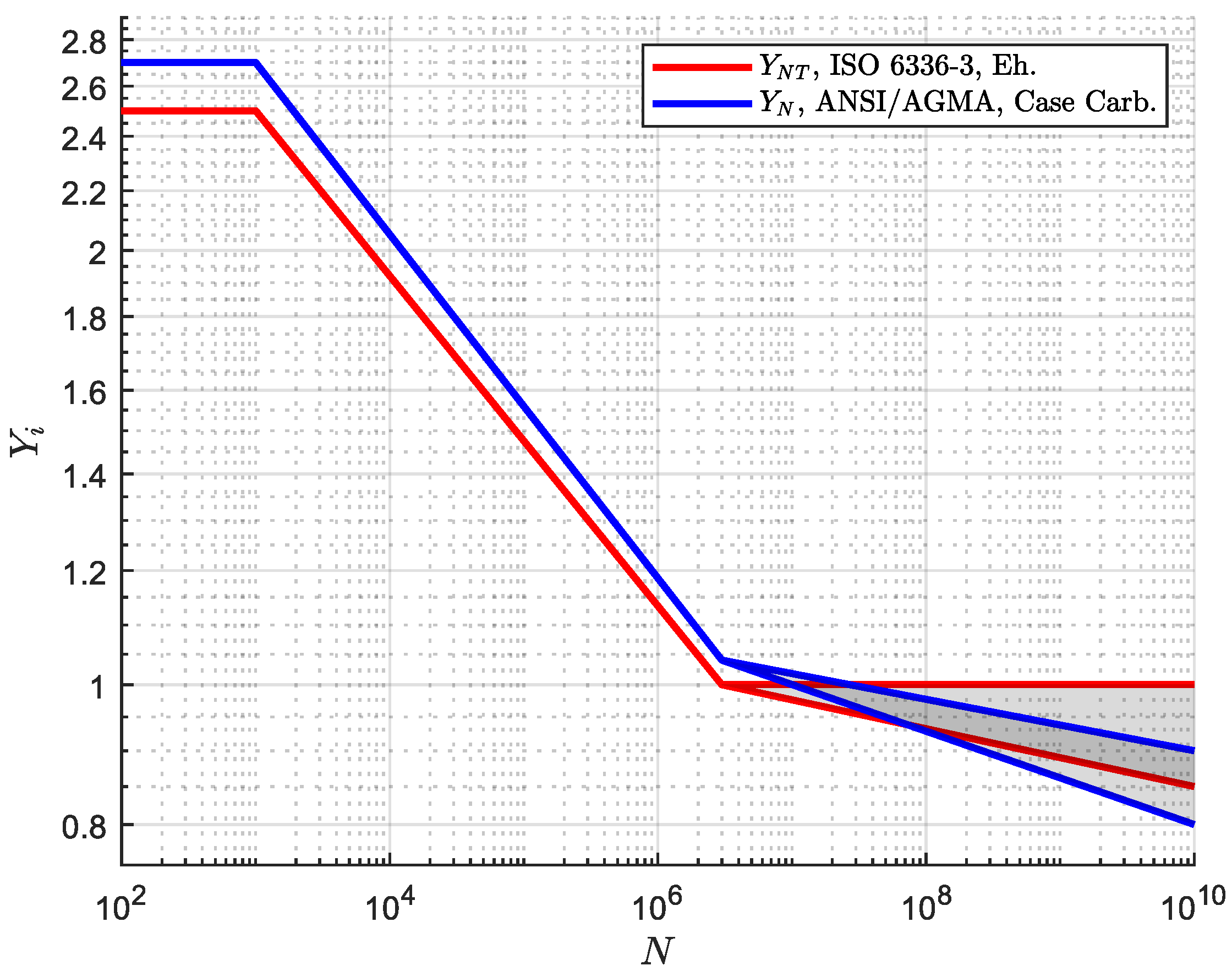
Figure 1. Typical shape of gear SN curve according to ISO 6336-3 [6] and ANSI AGMA 2001-D04 [7] considering tooth root bending for case-hardened gears.
Applsci 13 01546 g001
Figure 2. Pulsator test rig (schematic) adopted at FZG [36].
Applsci 13 01546 g002
Figure 3. The Schenck mechanical resonance pulsator adopted at POLIMI.
Applsci 13 01546 g003
Figure 4. SN curves for different failure probabilities by assumption of separated consideration of long-life (endurance) and limited-life ranges [24]. Extracted from AGMA 18FTM26, Reliability of Gears—Determination of Statistically Validated Material Strength Numbers, with the permission of the publisher, the AmericanGear Manufacturers Association, 1001 North Fairfax Street, Suite 500, Alexandria, Virginia 22314.
Applsci 13 01546 g004
Figure 5. Exemplary evaluation according to Hück staircase method; example extracted from [25].
Applsci 13 01546 g005
Figure 6. Logarithmic standard deviation considering failure load cycle numbers in limited-life range for peened gears according to Stahl [23].
Applsci 13 01546 g006
Figure 7. Evaluation of SN curves with different failure probabilities for exemplary campaign A from the experimental FZG database [24] according to FVA guideline 563 I [25].
Applsci 13 01546 g007
Figure 8. Evaluation of SN curves with different failure probabilities for exemplary campaign A from the experimental FZG database [24] according to the ML&SoE approach [27,28].
Applsci 13 01546 g008
Figure 9. Pulsator test database [24,27,28,56,65,66,67,68].
Applsci 13 01546 g009
Figure 10. Comparison of two estimation methods for exemplary campaign A from experimental FZG database [24].
Applsci 13 01546 g010
Figure 11. Comparison of the two estimation methods for exemplary campaign B from experimental FZG database [24,66].
Applsci 13 01546 g011
Figure 12. Comparison of the two estimation methods for exemplary campaign C from experimental FZG database [24].
Applsci 13 01546 g012
Figure 13. Comparison of the two estimation methods for exemplary campaign D from experimental FZG database [24] (Orig.) and excluding an outlier data point (Mod.).
Applsci 13 01546 g013
Figure 14. Comparison of the two estimation methods for exemplary campaign E from [27,28].
Applsci 13 01546 g014
Figure 15. Comparison of estimated k 1 (and its confidence interval) with its standardized equivalent.
Applsci 13 01546 g015
Figure 16. Comparison of estimated k 2 (and its confidence interval) with its standard equivalent.
Applsci 13 01546 g016
Figure 17. Trend of normalized s log σ F 0 confidence intervals.
Applsci 13 01546 g017
Table 1. Database reference summary.
YearReferenceShort Summary
2009[66]Presentation and analysis of a part of POLIMI points
2017[67]Presentation and analysis of a part of POLIMI points
2018[24]Partial statistical analysis of FZG points
2019[40]Presentation and discussion of selected FZG campaigns
2021[56]Partial statistical analysis of FZG points with focus on effects of materials and heat treatments properties
2022[65]Presentation and discussion of selected FZG campaigns
2021–2022[27,28]Presentation and analysis of a part of POLIMI points
Disclaimer/Publisher’s Note: The statements, opinions and data contained in all publications are solely those of the individual author(s) and contributor(s) and not of MDPI and/or the editor(s). MDPI and/or the editor(s) disclaim responsibility for any injury to people or property resulting from any ideas, methods, instructions or products referred to in the content.