Abstract
Structural expressionism resembles the use of slender structural elements, in particular beam-type elements. To satisfy structural, functional, and also architectural requirements a comprehensive structural analysis must be performed. The main issue of this study is the buckling analysis of beam-type elements, concerning Cavalieri’s principle. The present study is divided into two separate sections. The first part is a theoretical study, in which a variable cross-section beam-type element is modeled. The stability analysis is performed by an indirect variational method and the stiffness of the support connections is also introduced. The numerical simulation highlights 6 cases defined by the restraints of the support connections. The case study follows the modification of the critical buckling load of the variable cross-section beam-type element. Prior to the case study, a novel verification method is proposed to achieve a realistic cross-section for the beam-type element. The study revealed that with ideal characteristics of the stiffness coefficients of the restrains significant increase of the critical buckling load is obtained, and further if an actual situation is considered with finite values of the stiffness of the restrains, the variable cross-section for the beam-type element is a recommended and rational choice to make, to eliminate stability issues.
1. Introduction
1.1. General Aspects
The structural design process assumes achieving a structure that satisfies structural, functional, and architectural requirements, the famous triad formulated by Vitruvius in his multi-volume work De architectura in the 1st century BC. Due to the number of factors, one should consider parametric correlation rather than individual parameters, to perform an optimal structural design process, which in addition is an iterative one.
To quantify on a qualitative and quantitative scale the parameter correlation principle one may choose to evaluate the carbon footprint of a structure with the Life-cycle Assessment (LCA) technique [1]. Through this technique, one may have an overview of the most important stages during the life cycle of a structure, to take the most optimal solutions during the design phase. The design and structural conformation phase have an insignificant impact on the carbon footprint of a structure, on a quantitative scale, in comparison with the exploitation phase or the material production phase [2]. The structural design phase predefines the carbon footprint, on a qualitative scale, in the means that if a structure is completed further modifications would imply significant financial and time resources.
In the structural design phase, engineers tend to point out the most significant factors which in the end will define the final structure: strength, stability, and stiffness. The development of modern technologies and high-strength construction materials, allows architects and engineers to use a smaller number of elements, therefore the presence in particular of slender beam-type elements is more frequent.
The main goal is to avoid a structural collapse due to the loss of local or global stability, or by extensive deformation of structural elements. Both of these undesired failure types are closely related to structural topology, in other words, one must study the relations between different kinds of loads and the shape of the elements.
In order to achieve a comprehensive stability analysis and to compute the critical combination of the loading parameter, a gravity and a tip force parameter may be considered [3].
The main issue which is a debate for more than three centuries is the study of stability, in particular, the stability analysis of beam-type elements and frames, a bread-and-butter problem for structural engineers according to Z.P. Bažant. One of the first pioneers of the study of elastic buckling was Leonhard Euler who studied the strength and stability of centrally loaded structures, under their weight. Euler’s analytical formula denotes that failure would occur due to stresses induced by sidewise bending only, which is a particular case of long columns [4]. Since then the main preocupation of enginners’ is the study of beam-type elements with material and geometric nonlinearities. [5]. Euler’s studies have been followed by several significant theoretical contributions to the understanding of elastic buckling, but the fathers of modern engineering mechanics are considered to be S. Timoshenko and J.M. Gere who managed to write one of the most comprehensive guides to the elastic stability of structures [6].
Centrally loaded elements in a classical interpretation are considered to be beams and columns. Complex structures made up of beam-type elements with variable flexural rigidity are preferably used, in addition to the architectural and functional aspects, because it provides a better distribution of the strength and load. According to Euler’s formula, elastic buckling has a significant role in the design of elements with great height and large spans in the case of columns and of beams. Altogether beams do not carry a high amount of axial loads, but in the case of tensegrity type structures, one of the main concerns of the definition of structural topology is to reduce the length of isolated compressed elements [7]. The present research offers a different kind of approach for a specific situation, through a simple and high-precision method. The main purpose of the present study is to combine stability analysis with Cavalieri’s principle, in order to increase the critical buckling load, by modelling the geometric shape of the beam-type element.
1.2. Literature Overwiev
In recent years many analytical and numerical modells have been developed for the study of elastic buckling of structures. The feasible approach of elastic buckling has been proved to be the numerical modells. The majority of cases do not consider the variation of material and geometric properties. Arablis and Beskos proposed a new numerical method for the linear elastic stability analysis of plane structures consisting of beam-type elements. Throughout the analysis, the beams were considered with rectangular cross-sections with constant width and variable depth. The geometry is modeled through linearly tapered functions with constant width. The numerical modell implies the finite element method to compute the exact flexural and axial stiffness matrix and quasi-consistent mass and geometric matrices [8]. Das et al. proposed for the geometric shape of the beam-type elements linearly taper, exponential and parabolic functions, for which two types of cross-sections are adopted, solid circular and rectangular cross-sections. In the case of rectangular cross-sections, a constant width b is maintained [9].
The types of structural elements that are subjected to significant axial loads are the columns, which collect the weight of the structure and transfer it to the foundations. The columns have become more slender, due to architectural and design requirements [10]. Topological modelling of the beam-type element is a main issue regardless of the application field: from stability analysis to the study of dynamic behavior with plastic deformations [9]. In the case of slender columns with significant height, the establishment of the critical buckling load is an aspect of reference in the design phase. Gradually changing cross-sections ensures the decrease of the mass of the columns, which can be modelled throughout the moment of inertia of the cross-section [11].
Several studies investigate variable cross-section beam-type elements, in order to reduce the weight of the structure and increase strength, or to satisfy architectural requirements. The optimization process, through the structures own weight, is minimized and the critical buckling load is maximized, which is the main issue regarding variable cross-section beam-type elements [12]. Ruocco et al. [13] proposed an optimization problem to define the exact geometric shape of inhomogeneous columns with elastic restraints against buckling, loaded simultaneously with concentrated and distributed compressive loads which include self-weight. In this model, the Euler column is used, which is discretized by adopting the Hencky bar-chain model, in order to solve the differential equations which are governing the buckling phenomena. The critical bucking load, through this approach, represents the lowest eigenvalue of the resulting system of algebraic equations [13]. The Hencky bar-chain model offers a physical interpretation of the numerical finite difference method, as well as the possibility of optimization and buckling analysis of non-uniform beam-type elements [14].
Ruocco et al. offers a visual exemplification of Cavalieri’s principle, namely the optimized shape of the beam-type element is represented through parallel plan sections through lines, which are overlayed on the initial shape of the beam-type element, represented throughout the same technique, is order to highlight the topological modifications of the optimization process within the stability analysis [13]. Gual-Arnau uses the same technique in order to estimate the volume of a solid based on orthogonal parallel equidistant plane sections throughout lines [15]. Cavalieri’s principle has a high application rate in medicine, used in particular to estimate the volume of solids.
Eisenberg [16] conducted a stability analysis in the case of variable cross-section columns, with specific boundary conditions, loaded with variable axial compressive force. In his model, both the cross-section bending stiffness and the axial load variation are described through polynomial expressions, and the stiffness matrix for the member includes the effects of the axial loading [16]. The differential equation, which governs the phenomena, can be transformed into a system of algebraic equations with unknown coefficients. The buckling load is found as the load that makes the determinant of the stiffness matrix equal to zero [16].
The Variational Iteration Method (VIM) is a powerful method in the analysis of various engineering problems, and for solving nonlinear ordinary and partial differential equations and integral equations [17]. Coşkun and Atay applied VIM for the determination of critical buckling loads for Euler columns with constant and variable cross-sections. The study assumes various buckling cases with different boundary conditions and with different variations of cross-sections [17]. For the VIM exemplification method, there are presented a constant cross-section with an initial approximation of the linear ordinary differential equation is a cubic polynomial function with unknown coefficients. The variation of the cross-section is due to the variation of the moment of inertia of the column along the length of the Euler-type element. The material is assumed to be homogeneous therefore the variation of flexural rigidity depends only on the variation of the cross-section. There are proposed two variations of the flexural rigidity, thus exponential variation and by a power low, admitting a linear, a quadratic, and a cubic variation of the cross-section. The results are compared with the exact analytical solutions [17]. Das et al. used the variational method to define the static problem, in which the axial displacement field is to be computed [9].
Avcar [18] studied the elastic buckling of steel columns under axial compression with square, rectangle, and circular cross-sections, and different boundary conditions, i.e., fixed-free and pinned-pinned boundary conditions. For the solution along numerical computations, finite element modelling (FEM) has been employed. In this study, an analysis has been made regarding the effects of the boundary conditions, cross-sections, and slenderness ratios on the buckling loads of the steel columns [18]. Advanced numerical analysis can be performed with ANSYS Parametric Design Language codes, in order to determine the critical buckling loads. Saraçaoğlu and Uzun investigated circular variable cross-section concrete columns with a triangular variation of the cross-section admitting different ratios for the prismatic and the tronconic segments along the height of the columns. The analysis confirms that significant material economy and critical buckling load maximization can be obtained [12].
Abdel-Lateef et al. [11] proposed a theoretical elastic stability analysis of columns with variable cross-sections subjected to combined distributed and concentrated axial load. The minimization of the total potential energy technique is employed. The variation of the moment of inertia and the load intensity is governed by a power law of the distance along the column length. A simplified concept of the modified slenderness ratio is used to compute the critical stress for columns. The minimum potential energy principle is used to establish the necessary equations, which take into consideration the first two terms of the Fourier series for the deflection shape of the columns, which satisfies the geometric conditions [11].
Eisenberg suggested that one should not disregard the variation of non-dimensional critical buckling load with the variation of temperature field, which is a current research topic [19]. A localized differential quadrature method (LDQM) has a high potential to implement in the buckling analysis of axially graded non-uniform columns with elastic restraints. LDQM can be implemented for solving generalized eigenvalue problems with high accuracy and less computational effort [10].
2. General Approach of the Elastic Stability Issue in the Case of Beam-Type Elements
The property of elastic equilibrium of deformable bodies is considered their capability of recurrence to their initial state after small perturbations appear in the neighborhood of their equilibrium position. Under significant amounts of loads, beam-type elements can change their behavior. Behavior changes take place through the increase or decrease of their stiffness.
In some situations, the intensity of loads may reach critical values for which the system becomes unstable and may lose its load-bearing capacity for any slight increase in load intensity. At a critical state, if a lateral force is applied then a small deflection is produced. In an elastic analysis, the resulting deflection disappears when the lateral force is removed, thus the element returns to its initial form [20]. In the case of beam-type elements, significant compressive forces and bending moments may cause the loss of their elastic equilibrium configuration.
To evaluate on a quantitative and qualitative scale the effects of critical loads, the elastic equilibrium conditions must be formulated based on the final deformed shape of the structure, typical for stability issues and second-order theory [20]. The problem of elastic equilibrium of structures may be defined from three different perspectives, static methods, energy methods, and dynamic methods.
The definition of stability, through the dynamic approach, is fundamental and has an overview of all structural stability issues. Dynamic stability analysis is employed when structures are subjected to nonconservative loads, such as wind or pulsating forces. Throughout dynamic stability analysis, false equilibrium states can be identified, which can be caused by accelerated motions or vibrations with increasing amplitude. In modern structural engineering, the dynamic approach to stability is very important [20].
The static approach can be applied in the case of conservative structural systems, for which the critical loads can be computed, but cannot give a complete overview of the stability issue. Statics can only answer the question if the equilibrium state is stable or unstable. For simple structures, with no initial curvatures, it proves to be an effective method, but in the case of structures with imperfections, the energy approach is used to decide the stability of the system. Compared to the dynamic approach, it brings a great simplification [20].
The stability analysis of discretized elastic systems throughout the energy method is based on the Lagrange-Dirichlet theorem, which checks the positive definiteness of the energy function of the structure-load system. The energy criterion offers a comprehensive answer to the question of stability, which is given by the dynamic definition of stability for conservative systems [20].
The energy method can be applied for discrete and discretized systems, and for continuous structures. Continuous structures such as beam-type elements, which do not represent a discrete system, may usually be approximated by a discrete system, characterized by generalized displacements, which are kinematic variables [20]. Ramachandran and Gunguli used a discrete model in order to capture the onset of dynamic instability of statically determined columns [3].
3. Mathematical Modelling, Theoretical Aspects
3.1. Modelling Assumptions
In this study the following assumptions have been made: the material, of which the column is made, is linearly elastic; the hypothesis of small displacements and deformations; the axial force Q is constant and is computed through a first-order analysis;
- force Q is not influenced by the bending moments, it is a conservative force, which remains unchanged during bending; for the analysis the Euler-Bernoulli beam model is used, which does not take into account shear deformation and rotational bending effects as the Timoshenko-Ehrenfest beam theory; stiffness matrix assembling process neglects axial deformations; the beam-type elements are not subjected to lateral load, external loads are applied only in the joints; the column ax is perfectly straight, there are not taken into account any initial imperfections; no local buckling at any cross-section along the column length is allowed.
3.2. General Aspects
A major issue in the design of beam-type elements with significant axial loads is to improve the stability of the element and avoid their failure through buckling, which phenomenon threatens the structural integrity of the whole structural assembly. The phenomenon is more relevant in the case of statically determined structural assemblies.
The first step in the modelling of beam-type elements to improve their stability is to analyze Euler’s critical load derived in 1757, which is presented in Expression (1) [6].
In Expression (1) E represents Young’s modulus, denotes the minimum value of the moment of inertia of the cross-section, and represents the buckling length of the beam-type element subjected to compression forces, with respect to the imposed kinematic constraints to the joints.
Euler’s formula highlights two important aspects unaware of the kinematic restrains of the joints, the length of the element and the moment of inertia of the cross-section. The factor of direct proportionality with the critical load is the moment of inertia. This design parameter gain importance when the buckling modes are studied. The deflection shape associated with the primary buckling mode emphasizes potential critical areas of the element, which by similarity, can be scribed as potential areas of appearance of plastic hinges. In this manner it is required to amplify the value of the moment of inertia, therefore a variable cross-section beam-type element is obtained. In order to avoid sudden changes of the elements cross-section, which can be identified as stress concentration points, it is proposed the modelling of the cross-section of the element through a continuous function.
Modelling the cross-section of the element is performed with respect to Cavalieri’s principle. According to Cavalieri’s principle, the cross-section area of every section will remain unchanged during the modelling process, but the moment of inertia will change in accordance with the primary buckling mode. As a consequence of the mentioned principle, the elastic resistance of every cross-section is identical. Modelling a beam-type element with a variable cross-section follows the increase of the critical elastic buckling load, in an ideal case exceeding the elastic resistance of the cross-section, thus the buckling phenomenon can be avoided.
3.3. Modelling of the Moment Inertia
Modelling the moment of inertia of the cross-section presumes to assume a variation law. The variation law can be formed through interpolation functions between reference values in form of piecewise, multilinear, or polynomial functions. For the first two types of function, results are satisfying, although in the points where the function is not continuous the iterative process may be divergent, and the precision decreases by two orders of magnitudes. In the particular case of polynomial functions, the passing through the critical values is continuous, and the desired precision is in close correlation with the polynomial function degree.
The modelling of the moment of inertia in this study regardless of the kinematic constraints of the joints is performed with cubic functions, a piecewise polynomial formula known as the spline function. The natural boundary conditions are shown in Figure 1. Be f a function defined on which is interpolated in m + 1 nodes on n sub-intervals through a cubic interpolant S(x) defined in Figure 1.
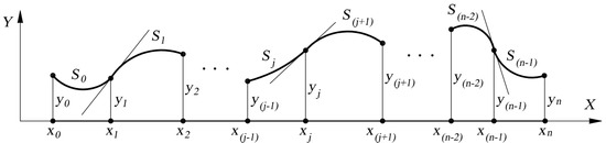
Figure 1.
Cubic interpolant , defined on sub-interval .
Cubic interpolant S(x), is a cubic polynomial piecewise function expressed in a general form as in Expression (2) [21].
In Expression (2), is defined on sub-interval . The boundary conditions for every sub-interval are presented in Relations (3a)–(3c).
The degree of the cubic interpolant is 3, , and the general expression for is presented in Expression (4) [21].
According to Expression (4), it is required to fix the values for coefficient , , and , with respect to the boundary conditions expressed in Relation (3a)–(3c). One of the cubic interpolant’s properties is to minimize the definite integral, presented in Expression (5), for every g function defined on an interval , which approximates function f through nods [21].
One can introduce notation , with respect to the general form presented in Expression (4), thus the boundary conditions from Relation (3a)–(3c) can be defined as recursive sequences, presented in Relation (6a)–(6c) [21].
The numerical value of coefficient results from the function evaluation of f at the input value of , denoted with , as for results from the function evaluation of f at the input value of , denoted with . For the recursive sequences from Relations (6a)–(6c) it is required the cubic interpolants coefficients as expressions which depends only on two specific arguments, thus coefficients and are chosen. Coefficient , can be expressed from Relation (6c), presented in Expression (7) [21].
Substituting Expression (7) in the recursive Sequence (6a,b), Expression (8a,b) can be expressed [21].
Substituting Expression (8a) in Expression (8b) it is possible to express coefficient with arguments and , as in Expression (9) [21].
The recursive Sequences (8b) and (9) can be expressed also for sub-interval , therefor Expression (8b) can be written as in Equation (10) [21].
Equation (10) represents m − 1 equations, and in order to solve a linear system of equations, two additional relations are required in the form of the natural boundary conditions expressed in Relation (11) [21].
Therefor the linear sytem of equations, whit respect to Equation (10) and Condition (11a,b), can be expressed as a matrix-vector Equation (12) [21].
In Equation (12), is the (m + 1) × (m + 1) coefficient matrix of the system whose implicit from is presented in Expression (13), is a vector made up of the m + 1 unknowns, presented in Expression (14a), and is the vector made up of the m + 1 right-hand sides of the equations, presented in Expression (14b).
Therefore, the solution of System (12) specifies the numerical values for coefficient . The cubic interpolant’s coefficients defined on n sub-intervals, are presented in Expressions (15a)–(15c) [21].
3.4. Stiffness Matrix Definition for Beam-Type Element with Elastic Restrains
The characterization of a structure or of an element from a structure, presented in Figure 2, through the geometric aspect, refers to the establishment of the deformed shape and defining the parameters which can define that specific deformed shape. The geometric characterization of structural elements highlights the fact that the deformed shape can be defined if the displacement field is known, displacements which can be translations or rotations. As a consequence of the geometric aspect, it is possible to choose the displacements as independent parameters to describe the elastic equilibrium state.
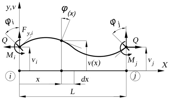
Figure 2.
The representation of a deformed beam-type element with nodal loads and displacements, where: L—is the length of the beam-type element; x—marks the distance to a current cross-section; dx—the incremental step between cross-sections; X—is the local reference system ax along the ax of the beam-type element; y—is the local reference system ax perpendicular to the beam-type element axes; v—denotes the general displacement of the cross-section; vi—is the displacement of the cross-section at joint i; vj—is the displacement of the cross-section at joint j; v(x)—is the displacement of the cross-section at position x; —is the rotation of cross-section at joint i; —is the rotation of cross-section at joint j; —is the rotation of cross-section at position x; Q—is the axial force; Mi—the bending moment at joint i; Mi—the bending moment at joint i; Fy,i—the sheer force at joint i.
The matrix-based formulation of the stability problem assumes the definition of the displacement field, which represents a function approximation problem. The task is to find a function that closely matches the displacement field. In the case of a bi-dimensional stability problem, for the beam-type element presented in Figure 2, the approximation problem assumes the approximation of the displacement field through a polynomial function of degree n − 1, presented in Expression (16).
In Expression (16), is the polynomial function which describes the displacement field, n − 1 = deg(v(x)) is the degree of , is a vector with the terms of the polynomial function divided by the terms’ coefficient; a vector with the polynomial functions coefficient. For joints and of the beam-type element, the kinematic boundary conditions can be written as in Relation (17).
The accuracy of the approximation of the displacement field depends on the degree of the chosen polynomial function. Therefore beside the 4 nodal parameters, there are introduced n − 4 non-nodal parameters . Consequently, the nodal displacement and force vectors for the beam-type element in Figure 2, are presented in Expressions (18) and (19) [22].
Expression (18) highlights the nodal and non-nodal parameters. Based on Expressions (18) and (19) the limit displacement boundary conditions are expressed in Equation (20).
The linear system of Equations presented in (20), is figured as a matrix equation in Equation (21).
In Equation (21), the matrix represents the coefficient matrix of the limit displacement boundary condition system. By expressing the vector of the polynomial function coefficients and by introducing it in Expression (16), the interpolation function matrix can be defined, as in Expression (22) and the polynomial function which describes the displacement field can be defined as in Expression (23).
In Expression (23), represents the nodal interpolation function matrix, which links the displacements of the beam-type element with the nodal displacements, is the vector of nodal and non-nodal displacements. Given Expression (23), Figure 3 is highlights the significance of non-nodal parameters/displacements through 4 interpolation functions of a degree n − 1 = 9 polynomial function.
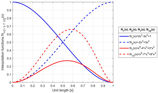
Figure 3.
Interpolation functions Nk(x), for k = [1 3 7 10].
Given Expression (23) and the geometric meaning of the differential relations between displacements, presented in Figure 4, the slope of the deflected beam axis , expressed in Expression (24), the strain , expressed in Expression (25), and the reaction forces induced in the beam-type element , expressed in Expression (26), can be defined as a function of nodal and non-nodal displacements .
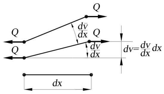
Figure 4.
Geometric representation of the differential relations between displacements, where dx—is the unit length of the beam-type element; dv—the unitary displacement; Q—the axial force.
In Expression (24), represents a matrix that links the slope of the deflected beam axis with the nodal and non-nodal displacement vector .
In Expression (25), represents the strain displacement matrix, which can define the curvature depending on the nodal and non-nodal displacements .
Expression (26) is based on the validity of Hooke’s law and the hypothesis of small displacements and deformations.
For the beam-type element, presented in Figure 2, the equilibrium is expressed through the principle of virtual work. According to the mentioned principle, the virtual displacements or the virtual forces are infinitesimal and consistent with the physical and elastic constraints of the beam-type element. Therefore for virtual displacements and the virtual forces, the same relations can be expressed as for the real displacements and forces, presented in Expression (27).
In Expression (27), is a vector of the nodal and non-nodal virtual displacements. The mathematical expression of the principle of virtual work is presented in Relation (28) [22].
In Relation (28), denotes the virtual mechanical work of the external forces, and represents the virtual mechanical work of the internal efforts. The mathematical expression of the virtual mechanical work of the external forces is presented in Expression (29).
In Expression (29), represents the virtual mechanical work of the external forces applied at the joints, denoted the virtual mechanical work of the axial force Q, presented in Figure 4. The virtual mechanical work of the external forces applied at the joints, can be expressed depending on the virtual nodal and non-nodal displacements, presented in Expression (30).
The virtual mechanical work of the axial force Q, in the case of an infinitesimal beam-type element of length dx, presented in Figure 4, is defined in Expression (31).
In Expression (31), the elementary virtual mechanical work of the axial force Q, can be expressed as in Expression (32).
By substituting Expression (32) in Expression (31) one can obtain the expression of the virtual mechanical work of the axial force Q, as a function of the nodal and non-nodal displacements, which is shown in Expression (33).
In Expression (33), represents the geometric stiffness matrix, which depends on the geometric characteristics of the beam-type element. The mathematical expression of the virtual mechanical work of the internal efforts is presented in Expression (34).
In Expression (34), represents the virtual mechanical work of the internal efforts, which is expressed in Expression (35), and represents the virtual mechanical work of the reaction forces of the support connections, presented in Expression (36).
In Expression (35), represents the material stiffness matrix of the beam-type element.
In Expression (36), denotes the value of the stiffness of the elastic support connections with respect to the kinematic boundary conditions, presented in Figure 5.
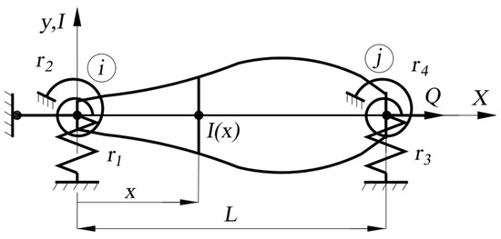
Figure 5.
Representation of the beam-type element with elastic support connections, where L—is the length of the beam-type element; x—marks the distance to a current cross-section; X—is the local reference system axes along the axes of the beam-type element; y—is the local reference system axes perpendicular to the beam-type element axes; I—the moment of inertia of the cross-section in a general form; I(x)—the moment of inertia of cross-section at section x; Q—is the axial force; r1—denotes the stiffness for a hindered transversal displacement for joint i; r2—denotes the stiffness for a hindered rotation for joint i; r3—denotes the stiffness for a hindered transversal displacement for joint j; r4—denotes the stiffness for a hindered rotation for joint j.
Expressions (35) and (36) are quadratic forms with nodal and non-nodal displacements as variables, therefor the stiffness coefficients can be obtained by the algebraic sum of the quadratic form’s coefficents, with respect to the connection indexes. Based on Expressions (35) and (36) the virtual mechanical work of the internal efforts can be written as in Expression (37).
With regard to Relationships (35) and (36), the procedure for assembling the material stiffness matrix, Expression (35) can be written as in Expression (37).
In Expression (37), denotes the assembled material stiffness matrix. Based on Relation (28) and Expression (29) Equation (38) can be expressed.
Equation (39) can be obtained by substituting Expresions (30), (33), and (37) in Equation (38).
Equation (39) must be fulfilled for every virtual displacement , therefore Equation (40) can be written.
A compact form of Equation (40) is presented in Equation (41).
In Equation (41), represents the elastic stiffness matrix of a beam-type element.
3.5. Formulation of the Stability Analysis
Based on Equation (41), internal forces , can be obtained with respect to the nodal and non-nodal displacements and the axial force Q. By expressing the nodal and non-nodal displacement vector from Equation (41), Expression (42) is obtained [23].
In Expression (42), represents the adjunct matrix of the elastic stiffness matrix, whose diagonal entries are the determinant of the elastic stiffness matrix . Based on Expression (42), the failure of a beam-type element occurs when there is an infinitesimal increase in the axial force the displacements tend to infinity. Therefore, in the case of beam-type elements, the loss of stability occurs when Equation (43) is satisfied, called an eigenvalue problem [23].
Equation (43), denotes the characteristic equation of the eigenvalue problem, which leads to a homogeneous system of equations, presented in Equation (44) [23].
The solution of the eigenvalue problem and of Equation (44), represents vector with the proper eigenvalues and the corresponding eigenvectors in a matrix . The minimum value of represents which denotes the critical buckling load, and the corresponding eigenvector the deflection shape.
3.6. Indirect Variational Method for the Study of the Conditions and Nature of Equilibrium
The potential energy is defined as a function of a function, that is, , a functional presented in Expression (45). The problem consists of determining the condition of the minimum functional of one function v of one variable x [20].
In Expression (45), v(x) is presumed to be continuous, with continuous first four derivates and also appropriate boundary conditions. The mathematical form of the total potential energy is presented in Expression (46) [23].
In Expression (46), U denotes the strain energy, V represents the potential of the external forces or the mechanical work of external force applied in joints. In this study, U is defined in Expression (47) through two energetic quantities.
It is assumed that the equilibrium position corresponds to an extreme value of the total potential energy, a condition presented in Equation (48) [23].
Equation (48) represents the condition for the Euler equation, with the proper boundary conditions. In mechanics, Equation (48) is generally equivalent to the equilibrium condition [23]. For the study of the nature of equilibrium, there are considered two stages of deformation, for the intensity λ of the axial force: stage 1, which is defined by displacements and total potential energy (,λ); stage 2, which corresponds to displacements ) + and total potential energy ( +).
The variation of the total potential energy by passing from stage 1 to stage 2 can be expressed in Expression (49) [23].
In Expression (49), is a continuous n-time differentiable function defined on the interval [0 L], which is expanded into a Taylor series, presented in Expression (50) [20].
In Expression (50), set the first-order derivative of the total potential energy, denotes the second-order derivative of the total potential energy and represents the higher-order derivative of the total potential energy, terms which are neglected in the modelling process [23].
The beam-type element in this study has a single degree of freedom v(x), which defines the system’s state. The terms obtained after the expansion into a Taylor series of , are presented in Expressions (51a)–(51c) [20].
With respect to the condition of equilibrium, presented in Equation (48), and to the fact that the potential of the external forces, for the case of constant loads, is expressed as , where represents a force associated with displacement , which is a linear displacement function, whose high-order derivative is canceled, the variation of the total potential energy between stage 1 and 2 is equivalent to the second-order derivative of the strain energy, presented in Expression (52) [20].
Expression (52) allows the study of the nature of equilibrium, as presented in Table 1.

Table 1.
Study of the nature of equilibrium according to the sign of [20].
In the case of neutral equilibrium, it is necessary to determine and study the higher-order derivative of the total potential energy according to Expression (50). The nature of equilibrium is indicated by the fourth-order derivative of the total potential energy, which has to be positive-definite, positive definiteness of guarantees stability [20].
Based on the first theorem of Castigliano the second-order derivative of the total potential energy with respect to the displacements represents the stiffness coefficient , which indicates a force at i due to unit displacement at j. According to this remark, Expression (52) can be expressed as in Expression (53) [23].
Expression (53) is a quadratic from in displacements, which in a matrix form is presented in Expression (54).
In Expression (54), is the displacement vector, is the elastic stiffness matrix of the studied structural element. Based on the condition that the variation of the total potential energy at the limit equilibrium state must be zero, respectively is obtained through the assembly of the material stiffness matrix and the geometric stiffness matrix, the equation of stability can be determined by an energetic method, which assumes an eigenvalue problem [23].
Continuous structures are analyzed through an indirect variational method, in which the structure is not discretized. The differential equations are obtained from the minimizing condition for the potential energy [20]. In contrast to this approach, the stability analysis, in which the structure is discrete or discretized and the expression of the second variation of potential energy is reduced to a quadratic form, is the direct variational approach [20].
3.7. Positive Definiteness of
The positive definiteness of guarantees stability. The total potential energy is quadratic from in displacements, and the elastic stiffness matrix [K] determines the quadratic form. Matrix [K] is a real symmetric matrix, which is positive-definite if and only if the eigenvalues of matrix [K] are positive [20].
The elastic stiffness matrix [K] is a real, Hermitian matrix and, according to Sylvester’s criterion, the necessary and sufficient condition for the quadratic from to be positive-definite if the leading principle minors are positive, meaning , where n represents the dimension of the real vector space of the elastic stiffness matrix, [24].
3.8. Boundary Conditions
According to the Lagrange-Dirichlet theorem, the equilibrium is stable if the total potential energy admits a local minimum. The condition that the potential energy must be strict minimum determines the differential equation which describes the problem and the admissible forms of the boundary conditions. The kinematic boundary conditions in mechanics or the essential boundary conditions in mathematics can be expressed in Relation (55) [20].
Equation (56a,b) can be used to express static boundary conditions in mechanics or natural boundary conditions in mathematics [20].
The approximate deflection shape v(x), or trial function, must always satisfy all the kinetic boundary conditions but does not have to satisfy the static boundary conditions. The static boundary conditions and the differential conditions of equilibrium are a result of the minimization of itself. If the static boundary conditions are satisfied, v(x) approximates the exact buckling shape, and the resulting critical load approximates more accurantely [20].
3.9. Rayleigh Quotient
The strain energy is a quadratic form in displacements and the neutral equilibrium state assumes that the second-order variation of the total potential energy is zero, conditions presented through a mathematical from in Equation (57) [16].
Based on Equation (48) and Expression (23), Equation (57) can be expressed as in Equation (58).
In Equation (58) represents the axial force multiplicator, which is expressed in Expression (59).
Expression (59) represents the Rayleigh quotient, which approximates the axial force, value dependent on the displacement field v(x). In order to fix the value of RQ, an iterative process must be launched which has as its starting value a certain displacement vector, a vector which readjusts after every iteration, with local convergence conditions. The defection shape at the moment of loss of equilibrium is not known, therefore the presented method is an approximative one [20].
According to the Lagrange-Dirichlet condition, the equilibrium is stable if P for every displacement v(x) compatible with the system’s kinematic constrains. At the limit state, the moment before the loss of stability, the critical buckling force represents , where it defines the number of iterations.
In Expression (59), the numerator represents the mechanical work of the internal efforts and the denominator the unitary mechanical work of the axial force, in this case, RQ, . Expression (59) for a beam-type element can be expressed as in Expression (60) [16].
In Expression (60), the Rayleigh quotient is defined as an analytic expression concerning the displacement field v(x), and function I(x) is a continuous function that describes the modification of the moment of inertia of the beam-type element [20].
3.10. Timoshenko Quotient
In the case of statically determined structures with the Timoshenko quotient, one may obtain a better approximation of the critical buckling load. The method assumes the appraisal of the strain energy on the basis of the bending moment M, which appears in the beam-type element due to deformation. The value of the bending moment is approximated with the product , instead of the curvature, which assumes an approximative displacement field [20].
In the case of a structure with linear elastic behavior, the strain energy is a quadratic form, and if it corresponds to the equilibrium position, then the modification of the total potential energy at the limit of equilibrium coincides with the potential energy. The modification of the total potential energy at the critical state must be equal to zero, a condition which can be expressed as in Equation (61) [20].
By expressing the axial force Q from Equation (61), Expression (62) is obtained [20].
The major advantage of the Timoshenko quotient is that it is a stationary value, a more precise value than the Rayleigh quotient.
4. Work Method
4.1. General Aspects
In this study, it is assumed that the beam-type element is part of a new structural assembly or part of a structure that requires structural rehabilitation. In the case of a new structure, a main structural design criterion is to use a minimum number of elements and a minimum amount of material. Therefore, the design or modelling of the beam-type element assumes an iterative process of optimization, through which the main goal is to fix the geometric characteristics of a beam-type element, of length L, subjected to axial force, with different kinematic constraints at the joints. In this study loads are applied only at the joints, therefore the state of strain is easier to control. The final failure criteria is a failure due to excessive stresses rather than buckling.
The modelling process assumes three interconnected iterative cycles, presented in Figure 6, which assumes obtaining a geometric configuration for the beam-type element which is not sensible to buckling.
The first iterative cycle has the purpose of fixing the maximum critical buckling load which can be achieved for a beam-type element with length L, by defining a variation function for the moment of inertia. To define the variation function of the moment of inertia, five coefficients are introduced which are associated with five equidistant points on the element, which indicate the variation of the moment of inertia as against the reference cross-section. The reference cross-section’s geometric and inertial characteristics are computed based on the imposed failure condition. At these points, the quantity of material is not modified, only its distribution on the cross-section. Between these reference points, cubic interpolation is performed in order to obtain a continuous function to express the variation of the moment of inertia.
The second iterative cycle starts after fixing the values for the five coefficients, which describe the variation of the moment of inertia, and the geometric properties of the reference cross-section. In the case of the 5 critical sections, it is important that the class of the sections be less than 4, in order to avoid the local verification process as described in SREN 1993-1-6. The third iterative cycle assumes verifying the failure condition, which presumes comparing the critical buckling load with the design resistance of the cross-section for uniform compression.
By undergoing the presented three iterative cycles, it is possible, with respect to the modelling assumptions, to fix the geometric characteristics for the beam-type element, with length L and variable cross-section, in order to achieve a favorable failure condition and avoid the loss of stability of the element.

Figure 6.
Flow chart of the work method.
Figure 6.
Flow chart of the work method.

The abbreviations in Figure 6 are related to a series of subprograms that incorporate the theoretical aspects from Section 3, as follows.
The subprogram entitled model_section_var sets the cubic interpolation function that describes the variation of the moment of inertia, as presented in Section 3. The input arguments are the length of the element L and the cross-section variation coefficients vector [i1 i2 i3 i4 i5]. The output for this program is the symbolic function Ii, which describes the modification of the moment of inertia.
The subprogram entitled sbc establishes the critical axial load, identified as the Rayleigh quotient, based on the variation of the cross-section, the material type, and the kinematic restraints imposed on the beam-type element. The input arguments are the length of the element L, the Young modulus E, the symbolic function Ii, and the stiffness vector for the joints. The outputs are the critical buckling force RQ and the deflection shape of the element through the displacement vector fp, which are the solution to the eigenvalue problem.
The subprogram entitled check_section is a verification program that calculates the geometric and inertial characteristics of the 5 critical sections and indicates if the class of the cross-section is greater than 3, based on the geometric characteristics of the reference cross-section. The input arguments are the cross-section variation coefficients vector, the outside diameter of the reference cross-section D0 and the thickness of the wall of the reference cross-section t0. The output of the program is a logical one. If the answer is TRUE then the variable cross-section beam-type element has no issues. When the answer is FALSE then modifications are required regarding the geometric entries of the reference cross-section or the variation coefficients of the moment of inertia.
The subprogram entitled failure_condition checks if the imposed failure condition is satisfied, regarding the failure due to the resistance of the cross-section for uniform compression rather than buckling. According to Hooke’s law, conditions can be expressed in terms of the area of the cross-section. The input arguments are the area of the reference cross-section A0, the steel-yield strength fy, and the critical buckling load RQ. The outputs are the elastic resistance of the cross-section Fc,Rd and the critical buckling load Fb,Rd.
4.2. Aspects Regarding the Input Data
4.2.1. Aspects Regarding the Length of the Beam-Type Element
The starting point of the modelling process is fixing the length of the beam-type element, L. The length of the element is a numerical value that remains constant during the iteration cycles and the kinematic constraints imposed on the joints.
In order to obtain a beam-type element with optimal shape from a topological point of view, the criteria regarding the variation of the cross-section are a necessary but not sufficient condition. The additional criteria are in close relation to Euler’s critical load, presented in Expression (1). In Expression (1), the second important factor which influences the critical buckling load is the length of the element, a numerical value that must be correlated with the geometric characteristics of the cross-section. Given the length of the element, a factor of inverse proportionality, there are three possible situations to note.
The possible situations are related to the effective geometric length of the element L and the critical length of the element , which is an ideal length for which the failure condition is fulfilled and the modelling of a variable cross-section makes sense.
In case I, the length of the element is less than the ideal length, or . In this case, the failure will occur by exceeding the value of the design resistance of the cross-section for uniform compression. The critical buckling force is net superior. In the present case, the modelling of a variable cross-section makes no sense, given the computational effort, the stiffness of the joints, and the technological terms. In this situation, the constant cross-section is an ideal solution.
In case II, the length of the element is quasi-equal to the ideal length, or . This case is considered the ideal case. The failure will occur by exceeding the value of the design resistance of the cross-section for uniform compression. The critical buckling force is superior. Modelling a variable cross-section is necessary in order to achieve a superior value for the critical buckling load beyond the design resistance of the cross-section for uniform compression.
In case III, the length of the element is greater than the ideal length, or . The failure will occur due to the loss of stability. The material is not used rationally.
For the cases for which the length of the element is a numerical value in the neighborhood of , there are several optimization methods, one of which is proposed in this study is to use a minimum quantity of material that has an optimum distribution on the cross-section.
4.2.2. Material Type and Section Profile
Slender structural elements subjected to a significant amount of compression forces appear to be characteristic of steel structural assemblies. In the case of steel structures, the beam-type elements are modeled according to the main stress in the cross-section. In the case of high axial forces, the most frequently used and recommended profiles are circular tubular profiles, with s-planes of sectional symmetry, with the inertial properties are equal in every direction. Given the boundary conditions for the beam-type element, circular tubular profiles are not sensible to flexural buckling. The recommended steel circular tubular profiles are presented in EN10219 [25]. In this study, these profiles will be considered as profiles for the reference cross-sections. The profile types presented in EN10219 are manufactured for constant cross-section elements. In this study, the reference cross-section id is presented in Expression (63), which indicates the geometric properties and material type for the cross-section.
In Expression (63) CHS is the abbreviation for the circular hole section, the type of profile chosen, D represents the external diameter in [mm], t the thickness of the profile’s wall in [mm], L represents the length of the beam-type element in [mm], S355JO is the grade of the steel, which carries a minimum yield strength of 355 [N/mm2], JO indicates that the steel has undergone longitudinal Charpy V-Notch impact testing at 27[J] at 0 [°C], EN10219 is the reference standard for the profile type [25].
4.2.3. The Stiffness of the Support Connections
In a theoretical study for the hindered displacements in a support connection, infinite value is associated with the stiffness of the connection. In the MATLAB programming language, the concept of infinity is associated with a numerical value of 101000 [26]. To quantify the effects of real support connections which allow small displacements there are imposed finite numerical values for the stiffnesses of the hindered displacements. In the case of other not constrained connections, their stiffness is not zero.
In this study, the numerical values imposed on the stiffnesses of the support connections are purely theoretical and they do not result from measurements on a physical model. In the theoretical model, the support connections are considered absolutely rigid or absolutely flexible. For any intermediate values of the rigidity of the elastic support, a flexible joint is obtained [6]. The modelling of elastic support connections resumes fixing the value of the stiffness for every connection type. The numerical values are computed based on the stiffness properties of the cross-section at the joints for the beam-type elements. For example, in the case of a beam-type element that is clamped-clamped the expression for the support connection stiffnesses, if one considers only the effect of bending, is presented in Expression (64) [27].
In Expression (64), E represents Young’s modulus, L represents the length of the element, denotes the moment of inertia at the joint cross-section. In Expression (64) for the first joint, it corresponds to the first and second values, the stiffness for a hindered transversal displacement and a hindered rotation of the joint, and for the second joint corresponds to the third and fourth value, the stiffness for a hindered transversal displacement and a hindered rotation of the joint. For every beam-type element, it is possible to fix a reference cross-section, which is considered the geometric invariant of the iterative process [27].
4.2.4. Aspects Regarding the Variation of the Cross-Section
The cubic interpolant describes the variation of the cross-section of the element on m sub-intervals. It is necessary to fix the values for the interpolation function at the limit of the sub-intervals, meaning m + 1 numerical values, indicated through coefficients . Due to rational considerations, the maximum modification for the moment of inertia of the cross-section is 100 [%] concerning the reference cross-section. The final values for the coefficients are fixed at the end of the iterative process. The modification of the moment of inertia assumes the modification of the outside diameter of the cross-section and the wall thickness of the cross-section .
In this study, the interpolation function, which describes the variation of the moment of inertia, is modeled on 4 sub-intervals. Therefore it is necessary to fix the value at five reference points, according to Expression (65).
4.3. Aspects Regarding Subprogram Check_Section
The potential points where it is recommended to modify the value of the moment of inertia are indicated by the defection shape of the compressed element. At the limits of m + 1 sub-intervals, the values of the moment of inertia get local maximum values. Subprogram Check_section determines the outside diameter of the cross-section and the wall thickness of the cross-section as a function of the reference cross-section. At the limit of a sub-interval, m Expression (66) can be written.
In Expression (66), denotes the numerical value of the reference cross-section, which is fixed for the constant cross-section beam-type element according to the imposed failure condition. The numerical value of parameter i is correlated with the amplitude of the deflection shape with respect to the kinematic boundary conditions.
Modelling the cross-section is based on Cavalieri’s principle. The area of the cross-section is equal for every cross-section, presented in Relation (67).
In Relation (67), represents the area of the reference cross-section, and it is highlighted the proposed modelling principle of the redistribution of material in the cross-section, highlighted also in Figure 7. The numerical value for every cross-section is fixed for the constant cross-section beam-type element according to the imposed failure condition.
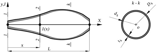
Figure 7.
Variable cross-section beam-type element, where L—is the length of the beam-type element; x—marks the distance to a current cross-section; X—is the local reference system axes along the axes of the beam-type element; y—is the local reference system axes perpendicular to the beam-type element axes; I—the moment of inertia of the cross-section in a general form; I(x)—the moment of inertia of the cross-section at section x; Dk—the outside diameter of the transversal cross-section k; dk—the inside diameter of the transversal cross-section k; tk—the thickness of the wall of transversal cross-section k; 0—the center of cross-section k-k.
In Figure 7 it is shown that a longitudinal and transversal cross-section of a variable cross-section beam-type element. Cross-section 1-1 corresponds to a section at the first joint, and cross-section 2-2 represents a current cross-section where a considerable modification of the moment of inertia is recorded. For cross-section 1-1 and cross-section 2-2 one may define the geometric and inertial characteristics presented in Expression (68a)–(68d).
In Expression (67), represents the area of the cross-section; denotes the moment of inertia of the cross-section; represents the outside diameter and represents the inside diameter of the cross-section, for . By substituting Expressions (68a)–(68d) into Expression (67) the system of Equations (69) is obtained, which can be expressed as in Equation (70) due to a computational artifice.
By substituting Equation (2) in Equation (1) from the system (70) and with Equation (2) from the System (71), is obtained.
If Equation (1) is gathered with Equation (2), from the system (71), than Equation (72) can be written, from which the outside diameter of cross-section 2-2 can be obtained as a function of the geometric characteristics of cross-section 1-1, concerning the modification of the moment of inertia, presented in Expression (73).
If Equation (2) is subtracted from Equation (1), from the system (71), Equation (74) can be written, from which the inside diameter of cross-section 2-2 can be obtained as a function of the geometric characteristics of cross-section 1-1, concerning the modification of the moment of inertia, presented in Expression (75).
If a ratio, p, is accepted between the outside and inside diameter of the cross-section for cross-section 1-1 Relation (76) can be written.
It is admitted the same ratio, p, between the outside and inside diameter of the cross-section for corss-section 1-1 Relation (77) can be written.
Expressions (78) and (79) are obtained by squaring Relation (76) and substituting the outside diameter for cross-section 1-1 in Expressions (73) and (75).
If Relation (77) is squared and Expressions (78) and (79) are substituted, Equation (80) is obtained.
The solution to Equation (80), with respect , highlights that the assumed ratio for both of the cross-sections is valid if the beam-type element has a constant cross-section. According to the reductio ad absurdum principlee, it is not possible to associate the same ratio for both of the cross-sections, therefore Relations (81) and (82) are written.
At this phase, the task is to determine ratio p2 as a function of ratio p1. Therefore by dividing Expression (78) with Expression (79) and based on Relation (82) the expression of ratio p2 can be expressed as in Expression (83).
To be able to control the modified cross-sections, the thickness of the profile wall of cross-section 2-2 is expressed as a function of the thickness of the profile wall of cross-section 1-1. Cross-section 1-1′s thickness of the profile wall can be expressed as in Equation (84).
From Equation (84) the inside diameter of secion 1–1, , can be expressed, which is introduced in Expressions (78) and (79) one may obtain Expressions (85) and (86).
If Expression (86) is substracted from Expression (85) the expression for the thickness of the profile’s wall for cross-section 2-2 is obtained, as a function of the thickness of cross-section 1-1′s profile wall and ratio p1, as in Expression (87).
Based on Expressions (85) and (87), the new sections can be controlled preliminary during the modelling phase, in order to define the class of the modified cross-section. By modifying the moment of inertia of the cross-section and by keeping constant the area, based on Cavalieri’s principle, the thickness of the profile’s wall will thin out. The iterative process must keep in mind this phenomenon, to avoid slender sections and to keep the class of the cross-section under 4, as to avoid further verification as presented in SREN 1993-1-6. By representing the buckling stress as a function of slenderness as in Figure 8, the target zone in this study is the shaded zone. The classification of the cross-section was performed as presented in SREN1993-1-1.
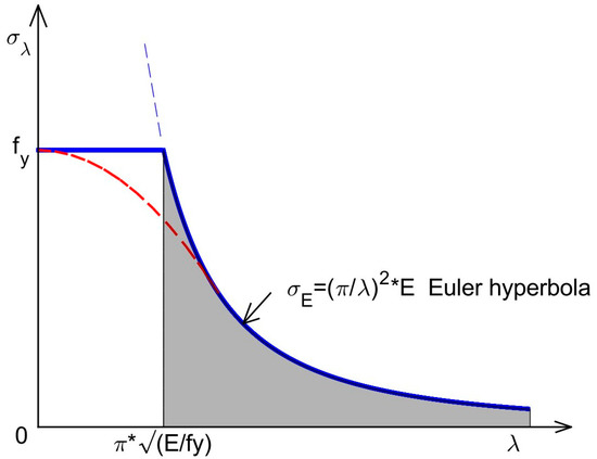
Figure 8.
Buckling stress as a function of slenderness, where λ-denotes the slenderness of the beam-type element; fy - the steel-yield strength; -the buckling stress; —the buckling stress as a function of the slenderness; E-Young’s modulus.
4.4. Aspects Regarding the Failure Condition
The optimization process assumes defining the configuration of the beam-type element through the moment of inertia of the cross-section in order to achieve a failure due to exceeding the design resistance of the cross-section under uniform compression rather than the design buckling resistance of the compression member. A limit state is characterized by appropriate values of the design resistances, which is a clear objective of the optimization process. The mentioned condition is expressed in a mathematical form as in Relation (88) [28].
In Relation (88), the symbols as in EN1993-1-1, represent the design resistance of the cross-section under uniform compression and represent the design buckling resistance of the compression member. The margin of error is considered 5 [%], and the empirical value, is quantified in Relation (88) by coefficient 1.05 [28].
4.5. Estimating the Error of the Iterative Process
The convergence criteria of the iterative process is to compute a numerical value for the critical buckling load which exceeds the value of the resistance of the cross-section under uniform compression, by modelling a variable cross-section for the beam-type element. To highlight the precision of the proposed method, a parameter is introduced to verify if the displacement field defined based on the defection shape of the beam-type element through the proposed method describes neutral equilibrium at critical load.
The definition of the control parameter, Error, is conditioned by the assumption that at the state of neutral equilibrium at critical load, the variation of the total potential energy is zero. The displacement field which describes the equilibrium state is approximated through a polynomial function. Therefore the variation of the total potential energy is not equal to zero. To quantify this amount of energy, it is related to the algebraic sum of the strain energy and the energy stored in the elastic support connection due to deformation. The mathematical form of the control parameter is presented in Expression (89).
If the numerical value of the control parameter, defined in Expression (89), is a small finite value, then axial force Q is appropriate to the critical buckling load.
4.6. Determining the Degree of the Polynomial Function v(x)
The displacement field is approximated through a polynomial function of degree n − 1. To fix the degree of the polynomial function, an analysis is performed on an axially loaded Euler column, a joint-supported statically determined system, for which the Rayleigh quotient and the Timoshenko quotient are calculated. This analysis is performed based on the first iteration cycle, with input values for the length of the element, Young’s modulus, and the moment of inertia of the reference cross-section unitary.
Based on the two methods of approximating the critical buckling loads, the analysis assumes the variation of the polynomial function’s degree until the numerical values for the critical buckling load are equal. The analysis is performed on an Euler column with a constant cross-section with results presented in Table 2 and on an Euler column with variable cross-section, with the coefficients which describe the variation of the moment of inertia , results presented in Table 3.
Table 2.
The results of the analysis for the constant cross-section Euler column.
In the case of the constant cross-section Euler column, the maximum error is 0.519%. The numerical values in Table 2 are presented in a graphical form in Figure 9.
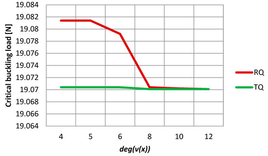
Figure 9.
The variation of the critical buckling force for the constant cross-section Euler column.
Based on the data from Table 2, for the constant cross-section Euler column, it is sufficient to model the displacement field through a polynomial function of degree eight.
In the case of the variable cross-section beam-type element, the maximum error is 0.573%. The numerical values in Table 3 are presented in a graphical form in Figure 10.
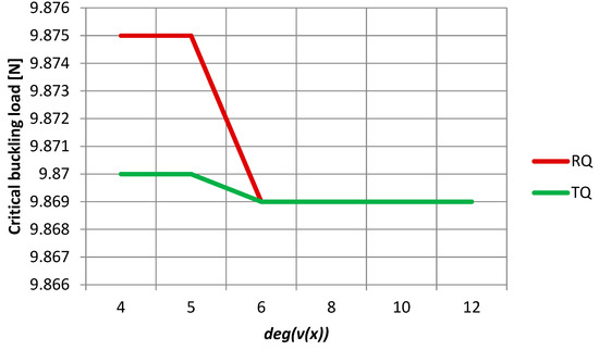
Figure 10.
The variation of the critical buckling force for a variable cross-section Euler column.
Based on the data from Table 3, for the variable cross-section Euler column, it is sufficient to model the displacement field through a polynomial function of degree six.
Table 3.
The results of the analysis for the variable cross-section Euler column.
Table 3.
The results of the analysis for the variable cross-section Euler column.
| deg(v(x)) | RQ [N] | TQ [N] | (RQ–TQ)·103 [N] |
|---|---|---|---|
| 12 | 19.0701 | 19.0701 | 0.0032 |
| 10 | 19.0702 | 19.0701 | 0.0276 |
| 8 | 19.0704 | 19.0701 | 0.2438 |
| 6 | 19.0792 | 19.0704 | 8.7387 |
| 5 | 19.0814 | 19.0704 | 10.9261 |
| 4 | 19.0814 | 19.0704 | 10.9261 |
4.7. Aspects Regarding the Modelling Phase concerning the Rayleigh Quotient
The approximation of the critical buckling load, through the Rayleigh quotient, presumes an iterative process through it is assumed a particular deflection shape, then after h iteration cycles, the critical buckling load is approximated concerning the modelling assumptions. The number of iteration cycles h is established based on the number of deflection shapes taken into account, through the moment of inertia of the cross-section.
In this study, it is assumed a particular variation of the moment of inertia of the cross-section, approximates the deflection shape of the beam-type element. By modifying the coefficients which describe the variation of the moment of inertia it is obtained a new defection shape, which is more appropriate to the real deflection shape, therefore the Rayleigh quotient decreases to a value more appropriate to the critical buckling load.
With the modification of the shape of the beam-type element, a new displacement field is obtained, and also the elastic stiffness matrix is changing therefore the critical buckling force increases. This is the basis of the first iterative cycle.
5. Case Study/Parametric Study/Computational Examples
The computational examples assume the study of statically determinate and indeterminate beam-type elements, six situations with ideal support connections, and also the consequence of the elastic support connections.
The starting point of every individual study is fixing the „reference” beam-type element, with a constant cross-section. The given element is modeled to achieve a critical buckling load superior to the resistance of the cross-section at uniform compression, explicitly to avoid the loss of stability.
The modelling of the beam-type element assumes knowing the kinematic boundary conditions. The kinematic boundary conditions in the case of ideal support connections can be defined as a zero displacement field. Regardless of the imposed kinematic boundary conditions the beam-type elements are considered with an equal geometric length of 6000 [mm], Young’s modulus of 2.1·105 [N/mm2], and yield strength of the steel, fy, with the value of 355 [N/mm2].
- a)
- The hinged-hinged beam-type element
The hinged-hinged beam-type element is presented in Figure 11a, which highlights the kinematic boundary conditions. The type of profile imposed on the reference cross-section is CHS163.8x8–6000–S355JO–EN10219, respectively values for the stiffness of the support connections are [inf 0 inf 0]. The results of the iterative optimization phase are presented in Table 4 and the graphical representation of the data from Table 4 is presented in Figure 12.
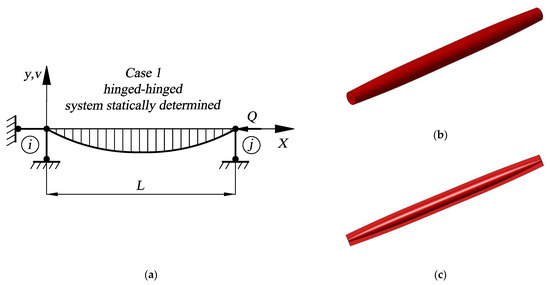
Figure 11.
The hinged-hinged beam-type element: (a) Schematic representation of the kinematic boundary conditions, where v—denotes the transversal displacement; Q—the axial force; (b) The variable cross-section beam-type element concering the imposed boundary conditions; (c) Longitudinal section of the modeled beam-type element which highlights the variation of the cross-section.
Table 4.
The data from the modelling process of the hinged-hinged beam-type element.
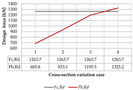
Figure 12.
The critical buckling force variation as against the resistance of the cross-section to uniform compression based on the data from Table 4.
In Table 4 as a function of the variation of the moment of inertia the resistance of the cross-section for uniform compression, Fc,Rd, and the buckling resistance, Fb,Rd, is computed and in the last column is presented the estimated error of the iteration cycle. The modeled hinged-hinged beam-type element is presented in Figure 11b,c.
In the case of the hinged-hinged beam-type element through the variation of the cross-section, without material addition, a significant increase of 93.23% for the critical buckling load is obtained and ensuring a proper failure condition as presented in Figure 12.
- b)
- The clamped-free beam-type element
The clamped-free beam-type element is presented in Figure 13a, which highlights the kinematic boundary conditions. The type of profile imposed on the reference cross-section is CHS323.9x12.5–6000–S355JO–EN10219, respectively values for the stiffness of the support connections are [inf inf 0 0]. The results of the iterative optimization phase are presented in Table 4 and the graphical representation of the data from Table 5 is presented in Figure 14.
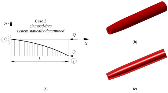
Figure 13.
The clamped-free beam-type element: (a) Schematic representation of the kinematic boundary conditions, where v—denotes the transversal displacement; Q—the axial force; (b) The variable cross-section beam-type element concerning the imposed boundary conditions; (c) Longitudinal section of the modeled beam-type element which highlights the variation of the cross-section.
Table 5.
The data from the modelling process of the clamped-free beam-type element.
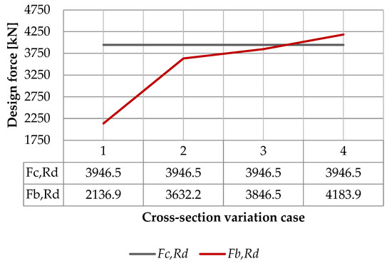
Figure 14.
The critical buckling force variation against the resistance of the cross-section to uniform compression based on the data from Table 5.
In Table 5 as a function of the variation of the moment of inertia the resistance of the cross-section for uniform compression, Fc,Rd, and the buckling resistance, Fb,Rd, is computed and in the last column is presented the estimated error of the iteration cycle. The modeled clamped-free beam-type element is presented in Figure 13b,c.
In the case of the clamped-free beam-type element through the variation of the cross-section, without material addition, a significant increase of 95.79% for the critical buckling load is obtained and ensuring a proper failure condition as presented in Figure 14.
- c)
- The guided-hinged beam-type element
The guided-hinged beam-type element is presented in Figure 15a, which highlights the kinematic boundary conditions. The type of profile imposed on the reference cross-section is CHS323.9x12.5–6000–S355JO–EN10219, respectively values for the stiffness of the support connections are [0 inf inf 0]. The results of the iterative optimization phase are presented in Table 6 and the graphical representation of the data from Table 6 is presented in Figure 16.
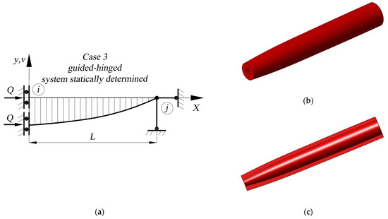
Figure 15.
The guided-hinged beam-type element: (a) Schematic representation of the kinematic boundary conditions, where v—denotes the transversal displacement; Q—the axial force; (b) The variable cross-section beam-type element concerning the imposed boundary conditions; (c) Longitudinal section of the modeled beam-type element which highlights the variation of the cross-section.
Table 6.
The data from the modelling process of the guided-hinged beam-type element.
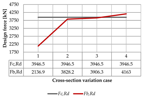
Figure 16.
The critical buckling force variation as against the resistance of the cross-section to uniform compression based on the data from Table 6.
In Table 6 as a function of the variation of the moment of inertia the resistance of the cross-section for uniform compression, Fc,Rd, and the buckling resistance, Fb,Rd, is computed and in the last column is presented the estimated error of the iteration cycle. The modeled guided-hinged beam-type element is presented in Figure 15b,c.
In the case of the guided-hinged beam-type element through the variation of the cross-section, without material addition, a significant increase of 94.81% for the critical buckling load is obtained and ensuring a proper failure condition as presented in Figure 16.
- d)
- The clamped-guided beam-type element
The clamped-guided beam-type element is presented in Figure 17a, which highlights the kinematic boundary conditions. The type of profile imposed on the reference cross-section is CHS193.7x8–6000–S355JO–EN10219, respectively values for the stiffness of the support connections are [inf inf 0 inf]. The results of the iterative optimization phase are presented in Table 7 and the graphical representation of the data from Table 7 is presented in Figure 18.
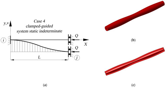
Figure 17.
The clamped-guided beam-type element: (a) Schematic representation of the kinematic boundary conditions, where v—denotes the transversal displacement; Q—the axial force; (b) The variable cross-section beam-type element concerning the imposed boundary conditions; (c) Longitudinal section of the modeled beam-type element which highlights the variation of the cross-section.
Table 7.
The data from the modelling process of the clamped-guided beam-type element.
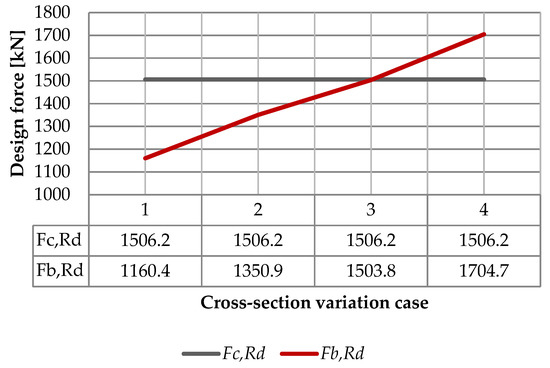
Figure 18.
The critical buckling force variation as against the resistance of the cross-section to uniform compression based on the data from Table 7.
In Table 7 as a function of the variation of the moment of inertia the resistance of the cross-section for uniform compression, Fc,Rd, and the buckling resistance, Fb,Rd, is computed and in the last column is presented the estimated error of the iteration cycle. The modeled clamped-guided beam-type element is presented in Figure 17b,c.
In the case of the clamped-guided beam-type element through the variation of the cross-section, without material addition, a significant increase of 46.91% for the critical buckling load is obtained and ensuring a proper failure condition as presented in Figure 18.
- e)
- The hinged-clamped beam-type element
The hinged-clamped beam-type element is presented in Figure 19a, which highlights the kinematic boundary conditions. The type of profile imposed on the reference cross-section is CHS127x5–6000–S355JO–EN10219, respectively values for the stiffness of the support connections are [inf 0 inf inf]. The results of the iterative optimization phase are presented in Table 8 and the graphical representation of the data from Table 8 is presented in Figure 20.
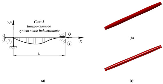
Figure 19.
The hinged-clamped beam-type element: (a) Schematic representation of the kinematic boundary conditions, where v—denotes the transversal displacement; Q—the axial force; (b) The variable cross-section beam-type element concerning the imposed boundary conditions; (c) Longitudinal section of the modeled beam-type element which highlights the variation of the cross-section.
Table 8.
The data from the modelling process of the hinged-clamped beam-type element.
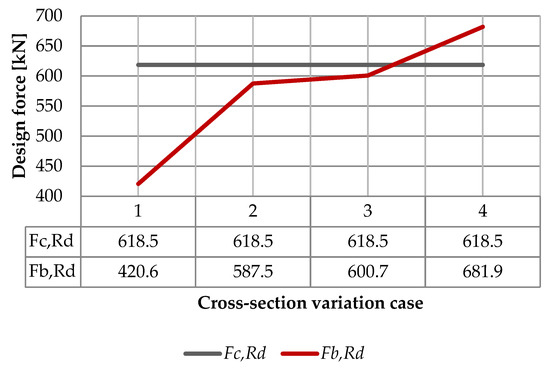
Figure 20.
The critical buckling force variation as against the resistance of the cross-section to uniform compression based on the data from Table 7.
In Table 8 as a function of the variation of the moment of inertia the resistance of the cross-section for uniform compression, Fc,Rd, and the buckling resistance, Fb,Rd, is computed and in the last column is presented the estimated error of the iteration cycle. The modeled hinged-clamped beam-type element is presented in Figure 19b,c.
In the case of the hinged-clamped beam-type element through the variation of the cross-section, without material addition, a significant increase of 62.13% for the critical buckling load is obtained and ensuring a proper failure condition as presented in Figure 20.
- f)
- The clamped-clamped beam-type element
The clamped-clamped beam-type element is presented in Figure 21a, which highlights the kinematic boundary conditions. The type of profile imposed on the reference cross-section is CHS101.6x6–6000–S355JO–EN10219, respectively values for the stiffness of the support connections are [inf inf inf inf]. The results of the iterative optimization phase are presented in Table 9 and the graphical representation of the data from Table 9 is presented in Figure 22.
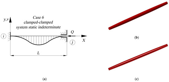
Figure 21.
The clamped-clamped beam-type element: (a) Schematic representation of the kinematic boundary conditions, where v—denotes the transversal displacement; Q—the axial force; (b) The variable cross-section beam-type element concerning the imposed boundary conditions; (c) Longitudinal section of the modeled beam-type element which highlights the variation of the cross-section.
Table 9.
The data from the modelling process of the clamped-clamped beam-type element.
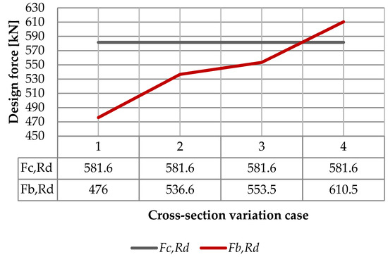
Figure 22.
The critical buckling force variation as against the resistance of the cross-section to uniform compression based on the data from Table 9.
In Table 9 as a function of the variation of the moment of inertia the resistance of the cross-section for uniform compression, Fc,Rd, and the buckling resistance, Fb,Rd, is computed and in the last column is presented the estimated error of the iteration cycle. The modeled clamped-clamped beam-type element is presented in Figure 21b,c.
In the case of the clamped-clamped beam-type element through the variation of the cross-section, without material addition, a significant increase of 28.25% for the critical buckling load is obtained and ensuring a proper failure condition as presented in Figure 22.
- g)
- The clamped-clamped beam-type element
The beam-type element with elastic supports is presented in Figure 23a, which highlights the kinematic boundary conditions. The type of profile imposed to the reference cross-section is CHS101.6x6–6000–S355JO–EN10219, respectively values for the stiffness of the support connections are [0.002 [kN/m] 28.935 [kNm/m] 0.002 [kN/m] 28.935 [kNm/m]]·104 established according to Expression (64). The results of the iterative optimization phase are presented in Table 10 for ideal and elastic restraints.
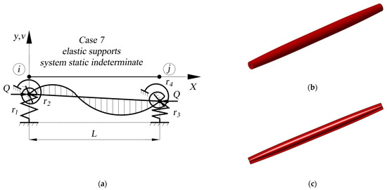
Figure 23.
The beam-type element with elastic supports: (a) Schematic representation of the kinematic boundary conditions, where L—is the length of the beam-type element; Q—is the axial force; r1—denotes the stiffness for a hindered transversal displacement for joint i; r2—denotes the stiffness for a hindered rotation for joint i; r3—denotes the stiffness for a hindered transversal displacement for joint j; r4—denotes the stiffness for a hindered rotation for joint j; (b) The variable cross-section beam-type element concerning the imposed boundary conditions; (c) Longitudinal section of the modeled beam-type element which highlights the variation of the cross-section.
Table 10.
The data from the modelling process of the beam-type element with elastic supports.
In Table 10, the symbol fin represents the finite numerical value for the corresponding stiffness of the elastic support, determined according to Expression (64). The symbol inf represents the ideal beam-type element support connections stiffness. In Table 10 it is highlighted that considering finite numerical values for the stiffness of the support connections the critical buckling load decreases radically, for example in case 1b the buckling force decreases by 84.07% and in case 2b buckling force decreases with 55.31%.
To avoid such sudden changes, which influence negatively the failure condition, another type of cross-section is chosen, with superior geometric and inertial characteristics. In Table 11 the data from modelling a beam-type element with elastic support is presented with the reference cross-section CHS139.7x6–6000–S355JO–EN10219, and the numerical values for the stiffness of the support connections [0.007 [kN/m] 78.996 [kNm/m] 0.007 [kN/m] 78.996 [kNm/m]]·104 determined according to Expression (64).
Table 11.
The data from the modelling process of the beam-type element with elastic supports with the new reference cross-section.
In Table 11 as a function of the variation of the moment of inertia the resistance of the cross-section for uniform compression, Fc,Rd, and the buckling resistance, Fb,Rd, is computed and in the last column is presented the estimated error of the iteration cycle.
In the case of the beam-type element with elastic supports through the modification of the cross-section, without material addition, a significant increase of 1725.05% for the critical buckling load is obtained as against the new reference cross-section beam-type element, and it is ensured a propper failure condition as presented in Figure 24. Figure 23b,c are presented the beam-type element with elastic supports. In Table 12 a comparison is presented of the critical buckling forces without and with elastic support, with the variation coefficients of the moment of inertial extracted from Table 10.
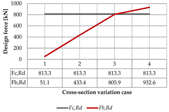
Figure 24.
The critical buckling force variation as against the resistance of the cross-section to uniform compression with respect to the data from Table 11.
Table 12.
The data comparison from the modelling process of the beam-type element without and with elastic supports.
Case 1b from Table 12 highlights the fact that by adding elastic supports the failure occurs due to the loss of stability and variation modelling a variable cross-section for the beam-type element is not appropriate and the reference cross-section with superior geometric and inertial properties is required.
Case 2b from Table 12 highlights that by adding elastic supports for a reference cross-section with superior geometric and inertial properties the failure occurs due to exceeding the resistance of the cross-section under uniform compression and variation modelling a variable cross-section for the beam-type element is necessary. Adopting elastic support instead of ideal support connections at least a 55% decrease is noticed in case of the critical buckling force.
The explanation for the radical decrease of the critical buckling force in the case of elastic support connections may be found in an analysis of the displacement field of a constant cross-section beam-type element loaded with axial forces and bending moments at the joints. In the case of the hinged-hinged beam-type element the displacements associated with the bending moment M, are proportional with M·L2 divided by the stiffness coefficient E·I, expressed in Relation (90a). The displacements associated with the axial force Q, are proportional with Q·L divided by the stiffness coefficient E·A, presented in Relation (90b) [29].
The quantities expressed in Relation (90a,b) have the same order of magnitude if conditions from Relation (91a,b) are satisfied, with respect to Brachmann-Landau notation [30].
For the quantities defined in Relation (91a,b), Relation (92) can be expressed, for a node in interval [29].
By expressing ratio M/Q from Relation (92) with respect to Hooke’s law and Navier’s relation, Expression (93) is obtained [31].
In Relation (93), represents stress associated with the bending moment, represents the stress associated with the axial load, and for a tubular circular cross-section ratio, I/W is equal to a maximal distance of section point from the neutral axis that crosses the centroid, in the present situation it represents the half of the outside diameter of the profile, D, which leads to Relation (93) and thus Relation (94) [29].
The right part of the Relation (94) represents a considerably small ratio, representing the ratio between the outside diameter and the length of the element, therefore has the same order of magnitude compared to . Based on the mathematical relation of the Euler-Bernoulli beam theory, Relation (94) can be expressed as Relation (95) [29].
In Relation (95) serve as the maximal strain associated with the bending moment and denote the strain associated with the axial load. Based on the expression of the maximal strain of the cross-section, ε, Expression (96) is obtained [29].
In Relation (96) is highlighted the influence of strain associated with the bending moment on the displacement field of the beam-type element, with in this case is practically insignificant. In this manner by adding elastic support connections with finite values for the stiffnesses, computed based on the Expression (64), regardless of the imposed boundary conditions, the beam-type element’s behavior is practically identical to the Euler column.
The method through the ideal support connection is replaced with elastic support connection, with finite numerical values for the stiffness coefficients computed based on the deformability of the structural assembly, must consider the fact that the numerical value of the critical buckling load can be half as computed. To better understand the phenomena, one can make an analogy with a planer truss with rigid nodes and structural assemblies with high statical indeterminacy, due to the axial strain of the structural elements, in the joints of the beam-type elements bending moments will occur as a function of the relative rotation of the trusses, an effect which has been proven to be a secondary one.
6. Conclusions
6.1. Aspects Referring to the Precision of the Proposed Method
The first important aspect which needs to be highlighted is the high precision of the proposed method, which approximates the critical buckling load for the case of a beam-type element with a variable cross-section. The high precision is in the first place to the adopted methodology, more precisely by adopting a cubic interpolant to express the variation of the cross-section and by modelling the displacement field through a polynomial function with a degree greater than five. Secondly, it is possible to achieve such precision due to the numerical properties of an irrational number, which is closely related to Expression (1), Euler’s critical buckling load. In Expression (1) the irrational number appears which decimal representation never ends, respectively its decimals do not enter a permanently repeating pattern. This property makes it possible to estimate with high accuracy the variation of the total potential energy at neutral equilibrium at critical load.
6.2. The Influence of the Statical Determinacy of the Structural Element
The case study represents a numerical but especially analytical analysis, which is a different kind of approach for stability analysis. It assumes linking two theories, namely Cavalieri’s principle and elastic buckling theory, in order to perform a comprehensive stability analysis in the elastic domain to increase the elastic buckling load for the beam-type element, through geometric modelling of the cross-section for the beam-type elements, with specific boundary conditions.
The case study ranges from statically determinate to statically indeterminate structural elements, concerning the imposed kinematic boundary conditions. In the case of statically indeterminate structural assemblies, it is not possible to establish a unique numerical value for the stress ratios of the elements, due to the fact that modifying the axial stiffness of an element influences the stress redistribution in the whole structure. In the case of statically determined structural assemblies, it is possible to compute a unique value for the unitary efforts in the structural elements. The case study has proven that in the case of statically determinate structural elements have achieved the highest increase of the critical buckling load. The final result in therm of the achieved increase rates is presented in Figure 25.
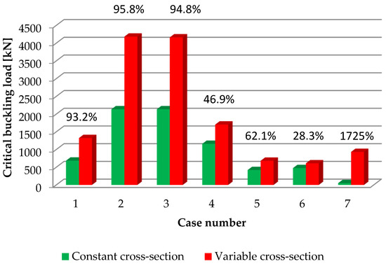
Figure 25.
The increase of the critical buckling load for the beam-type element concerning the imposed kinematic boundary conditions.
A very important result is highlighted in Figure 25 for the beam-type element with elastic supports. The elastic support connections modify significantly the behavior of the structural element under axial loads and influence excessively the critical buckling load. In the case of constant cross-sections increasing the area of the cross-section is not a rational solution and a favorable failure condition is practically impossible to achieve. Modelling a variable cross-section beam-type element is a practical solution to increase the critical buckling load above the value of the resistance of the cross-section subjected to uniform compression. A correct modelling of the shape of the beam-type element, through the moment of inertia, may point to a considerable increase of the critical buckling load, up to 1725% in the present case as against the constant cross-section, with respect to Cavalieri’s principle. A very important aspect is that by imposing elastic support connections instead of ideal ones the critical buckling load is influenced and a significant decrease is observed, up to at least 55% in the studied case. This remark is very important for structural engineers when they establish the geometric and inertial characteristics of a structural element subjected to considerable axial load.
A certain fact is that statically determinate structures have lack of structural redundancy, but the state of stress and strain can be easily controlled through the whole elastic behavior domain of the beam-type element. By adopting beam-type elements with variable cross-sections it is possible to fix significant numerical values for the length of the elements, with respect to the secondary effects of the rigid joints.
Based on the presented aspects the adopted beam-type elements with variable cross-sections are recommended in the case of high-span planar or spatial trusses. The mentioned structural assemblies must be statically determinate, made up of a minimum number of elements, with significant length, and using high-quality materials.
6.3. Aspects Regarding the Common Undesired Failure Conditions
The failure of a structural assembly and in essence structural elements must take place with a high amount of warning signs which enables the evacuation of persons and material goods from the potentially affected area. In this manner, there must be warning signs, easily to be identified. Due to the state of stress and strain in the structural elements, the elements failure can occur without any warning signs. The undesired failure types are considered failure through compression, shear force, torsion, and buckling.
In some particular situations, due to the topology of the structural assembly, the structural elements are subjected to a state of stress and strain due to other types of loads than has been expected at the structural design phase. In the case of beam-type elements, compression forces can lead to unexpected failure, due to the joints which are considered potential tension concentrators. The failure through shear forces and torsion are in close relation with the state of stress and strain in the structural element, respectively to avoid them one can take actions on a local scale regarding the design of the structural element. The measures include adopting appropriate cross-sections and quantities of materials. The loss of stability due to extensive axial loads is high in the case of slender beam-type elements. To avoid the present phenomena the critical buckling load must be increased above the value of the elastic resistance of the cross-section. This is possible by modelling beam-type elements with variable cross-sections and by designing statically determinate structural assemblies for which the state of stress and strain can be computed uniquely and using high-quality materials.
Author Contributions
Conceptualization, M.B. and L.I.; methodology, M.B.; software, M.B.; validation, L.I.; formal analysis, L.I.; investigation, L.I.; resources, M.C.; data curation, M.B.; writing—original draft preparation, L.I.; writing—review and editing, L.I. and M.C.; visualization, M.C.; supervision, M.B.; project administration, M.B. All authors have read and agreed to the published version of the manuscript.
Funding
This research received no external funding.
Institutional Review Board Statement
Not applicable.
Informed Consent Statement
Not applicable.
Data Availability Statement
Not applicable.
Conflicts of Interest
The authors declare no conflict of interest. The funders had no role in the design of the study; in the collection, analyses, or interpretation of data; in the writing of the manuscript; or in the decision to publish the results.
References
- Sun, H.; Park, Y. Emission Calculation Method during Construction Process for Developing BIM-Based Performance Evaluation System. Appl. Sci. 2020, 10, 5587. [Google Scholar] [CrossRef]
- Gong, Y.; Song, D. Cycle Building Carbon Emissions Assessment and Driving Factors Decomposition Analysis Based on LMDI—A Case Study of Wuhan City in China. Sustainability 2015, 7, 16670–16686. [Google Scholar] [CrossRef]
- Ramachandran, N.; Gunguli, R. Family of columns isospectral to gravity-loaded columns with tip force: A discrete approach. J. Sound Vib. 2018, 423, 421–441. Available online: https://www.sciencedirect.com/science/article/abs/pii/S0022460X18301536 (accessed on 4 January 2023). [CrossRef]
- Scholarly Commons. Available online: https://scholarlycommons.pacific.edu/euler-works/238/ (accessed on 12 August 2022).
- Bjorhovde, R. Evolution and State-Of-The-Art of Column Stability Criteria. J. Civ. Eng. Manag. 2010, 16, 159–165. [Google Scholar] [CrossRef]
- Timoshenko, S.P.; Gere, J.M. Theory of Elastic Stability, 2nd ed.; Dover Publication, Inc.: New York, NY, USA, 2010; pp. 46–158. [Google Scholar]
- Botis, M.F.; Imre, L.; Cerbu, C. Computer-aided design of a tensegrity structure. Structures 2022, 38, 340–360. [Google Scholar] [CrossRef]
- Karabalis, D.L.; Beskos, D.E. Static, dynamic and stability analysis of structures composed of tapered beams. Comput. Struct. 1983, 16, 731–748. [Google Scholar] [CrossRef]
- Das, D.; Sahoo, P.; Saha, K. Dynamic analysis of non-uniform taper bars in post-elastic regime under body force loading. Appl. Math. Model. 2009, 33, 4163–4183. Available online: https://www.sciencedirect.com/science/article/pii/S0307904X09000584 (accessed on 4 January 2023). [CrossRef]
- Yilmaz, Y.; Girgin, Z.; Evran, S. Bucling Analyses of Axially Functionally Graded Nonuniform Columns with Elastic Restraint Using a Localized Differential Quadrature Method. Math. Probl. Eng. 2013, 2013, 1–12. [Google Scholar] [CrossRef]
- Abdel-Lateef, T.H.; Dabaon, M.A.; Abdel-Moez, O.M.; Salama, M.I. Buckling Loads of Columns with Gradually changing Cross-Section subjected to Combined Axial Loading. In Proceedings of the Fourth Alexandria International Conference on Structural and Geotechnical Engineering, Alexandria, Egypt, 2–4 April 2001. [Google Scholar]
- Saraçaoğlu, M.H.; Uzun, S. Stability analysis of columns with variable cross-sections. J. Struct. Eng. Appl. Mech. 2020, 3, 169–179. [Google Scholar] [CrossRef]
- Ruocco, E.; Wang, C.M.; Zhang, H.; Challamel, N. An approximate model for optimizing Bernoulli columns against buckling. Eng. Struct. 2017, 141, 316–327. [Google Scholar] [CrossRef]
- Ruocco, E.; Zhang, H.; Wang, C.M. Hencky bar-chain model for buckling analysis of non-uniform columns. Structures 2016, 6, 73–84. Available online: https://www.sciencedirect.com/science/article/abs/pii/S2352012416000187 (accessed on 4 January 2023). [CrossRef]
- Gual-Arnau, X. On the Volume form Planar Sections Through a Curve. Image Anal. Stereol. 2005, 24, 35–40. [Google Scholar] [CrossRef]
- Eisenberger, M. Buckling loads for variable cross-section members with variable axial forces. Int. J. Solids Struct. 1991, 27, 135–143. [Google Scholar] [CrossRef]
- Coşkun, S.B.; Atay, M.T. Determination of critical bucling load for elstic columns of constant and variable cross-sections unsing variational iteration method. Comput. Math. Appl. 2009, 58, 2260–2266. [Google Scholar] [CrossRef]
- Avcar, M. Elastic Buckling of Steel Columns Under Axial Compression. Am. J. Civ. Eng. 2004, 2, 102–108. [Google Scholar] [CrossRef]
- Eisenberger, M. Buckling loads for variable cross section bars in a nonuniform thermal field. Mech. Res. Commun. 1992, 19, 259–266. [Google Scholar] [CrossRef]
- Bažant, Z.P.; Cedolin, L. Stability of Structures Elastic, Inelastic, Fracture and Damage Theories; World Scientific Co., Pte. Ltd.: Singapore, 2010; pp. 3–369. [Google Scholar]
- Math 541—Numerical Analysis. Available online: https://jmahaffy.sdsu.edu/courses/s10/math541/index.htm (accessed on 26 June 2022).
- Dósa, A.; Popa, L. High order beam elements for the stability and non-linear analysis of frame structures. In Proceedings of the Computational Civil Engineering 2006 International Symposium, Iași, Romania, 26 May 2006. [Google Scholar]
- Bănuț, V.; Teodorescu, M.E. Calculul Geometric Neliniar al Structurilor de Rezistență; Editura Conspres: Bucharest, Romania, 2010; pp. 141–163. [Google Scholar]
- Radomir, I.; Purcaru, M.A.P.; Fulga, A. Matematici Superioare Pentru Ingineri; Editura Universității ”Transilvania”: Brașov, Romania, 2009; Volume I, pp. 34–132. [Google Scholar]
- EN 10219; Cold Formed Welded Structural Hollow Sections of Non-Alloy and Fine Grain Steels. CEN-European Commitiee for Standardization: Brussels, Belgium, 2006.
- MathWorks. Available online: https://www.mathworks.com (accessed on 25 August 2022).
- Gheorghiu, A.A. Statica Construcțiilor Ii. Structuri Static Nedeterminate; Editura Tehnică: Bucharest, Romania, 1965; pp. 487–682. [Google Scholar]
- EN 1993; Eurocode 3: Design of Steel Structures. CEN—European Commitiee for Standardization: Brussels, Belgium, 2005.
- Feodosiev, V.I. Advanced Stress and Stability Analysis. Series: Foundations of Engineering Mechanics; Springer Verlag GmbH: Heildelberg, Germany, 2005; pp. 175–177. [Google Scholar] [CrossRef]
- Stănășilă, O. Analiză Matematică; Fundația Floarea Darului: Bucharest, Romania, 2014; pp. 79–86. [Google Scholar]
- Timoshenko, S.P. Strength of materials. Part ii. Advanced Theory and Problems, 3rd ed.; CBS Publishers & Distributiors Pvt. Ltd.: New Delhi, India, 2002; pp. 1–69, 145–173. [Google Scholar]


Disclaimer/Publisher’s Note: The statements, opinions and data contained in all publications are solely those of the individual author(s) and contributor(s) and not of MDPI and/or the editor(s). MDPI and/or the editor(s) disclaim responsibility for any injury to people or property resulting from any ideas, methods, instructions or products referred to in the content. |
© 2023 by the authors. Licensee MDPI, Basel, Switzerland. This article is an open access article distributed under the terms and conditions of the Creative Commons Attribution (CC BY) license (https://creativecommons.org/licenses/by/4.0/).