Consistency of Imperfections in Steel Eurocodes

Abstract

The second-order theory was used to analyze the flexural buckling of an individual member simply supported on both member ends, with a uniform double symmetric cross-section under a uniform axial force in an elastic state. The purpose was to show the influence of four different amplitudes of initial imperfections on the shape of the elastic buckling mode ${\eta }_{\mathrm{cr}}\left(x\right)$ used in the current EN 1993-1-1 and its new draft, prEN 1993-1-1. Three methods were followed for the analysis: the equivalent member (EM) method, the unique global and local initial (UGLI) imperfection method, and second-order theory with the initial imperfection having an initial local bow imperfection $e_0$. For the relevant quantities, simple formulae were derived and their distribution was drawn on diagrams to represent their graphical interpretations for the first time ever. The formulae and diagrams were valid for the ultimate limit state, which means $N_{\mathrm{Ed}}=N_{\mathrm{b},\mathrm{Rd}}.$ The influence of four different amplitude values was evaluated: (a) $e_{0,\mathrm{k}}$, proposed for the UGLI imperfection method in the draft EN 1993-1-1; (b) the initial local bow imperfection $e_0$, utilized in the current EN 1993-1-1; (c) the other one employed in its draft; and (d) $e_{0,\mathrm{d}}$, used in the UGLI imperfection method in the current EN 1993-1-1, the current EN 1999-1-1, and the draft prEN 1999-1-1. The main conclusion was that $e_{0,\mathrm{k}}$ must not be used in the draft EN 1993-1-1. The UGLI imperfection method was also applied to the column fixed at one end and simply supported at the other end. This example showed the geometrical interpretation of relevant amplitudes. The historical development of the UGLI imperfection method is also presented. All the relations are illustrated in two numerical examples, and the geometrical interpretations of formulae were used in the diagrams. The partial results were verified by the independent computer programs FE-STAB and IQ 100.

1. Introduction

The causes of imperfections of members may include the following: (a) a deviation from straightness and twist; (b) unavoidable eccentricity due to variation in the cross-sectional dimension; (c) eccentricity due to non-centric loads; (d) a residual stress pattern; etc. All these causes can be explained by an equivalent geometrical imperfection, which is defined by its shape and amplitude.

The shape of the equivalent geometrical imperfection in EN 1993 (Part 1-1) was chosen as the elastic buckling mode ${\eta }_{\mathrm{cr}}\left(x\right)$ of the structure, i.e., for the simply supported column ${\eta }_{\mathrm{cr}}\left(x\right)\sin \left(\pi x/L\right)$, because then ${\eta }_{\mathrm{cr}}\left(x\right)$ and the deformation from the compression force $N_{\mathrm{Ed}}$ would be affine. This fact simplifies both the calculation and result. The bending moment $M_{\mathrm{Ed}}^{\mathrm{II}}=N_{\mathrm{Ed}}{\eta }_{\mathrm{tot},\mathrm{c}}$ is only of interest at the midspan of the column because the compression force and the cross-section are uniform along the column length.

Four different amplitudes appear in EN 1993 (Part 1-1): (a) amplitude $e_{0,\mathrm{k}}$, hidden in the reduction factor $\chi$ of the equivalent member (EM) method; (b) an initial local bow imperfection $e_0$ in the current EN 1993-1-1; (c) the other one in the new draft, prEN 1993-1-1; and (d) amplitude $e_{0,\mathrm{d}}$, used in the UGLI imperfection method.

To show the differences caused by the various amplitudes used in the different methods, a decision was made to investigate individual members simply supported on both member ends with uniform double symmetric cross-sections under a uniform axial force in an elastic state.

The following methods show how the stability of an individual member under compression can be checked:

(a)

The EM method;

(b)

The UGLI imperfection method, which is the second-order analysis of a member under compression with a unique global and local initial (UGLI) imperfection;

(c)

The second-order analysis of a member under compression, with a shape imperfection that is derived from the elastic buckling mode of the structure with an amplitude $e_0$ of the equivalent geometrical bow imperfection.

All these methods are described. For the relevant quantities, formulae are given together with their geometrical interpretations, which may be useful for designers and educational institutes. The old and new Eurocode initial local bow imperfections $e_0$ were compared to one another, and also to the $e_{0,\mathrm{k}}$ and $e_{0,\mathrm{d}}$ values. It was shown that the decision made in the new prEN 1993-1-1, namely to use $e_{0,\mathrm{k}}$ in the UGLI imperfection method (in fact, safety factor ${\gamma }_{\mathrm{M}1}$ was removed from the $e_{0,\mathrm{d}}$ used in the current EN 1993-1-1), has important negative consequences. It was also proven that the procedure followed in the current EN 1993-1-1, EN 1999-1-1, and the draft prEN 1999-1-1, and that used in the UGLI imperfection method, gives an $e_{0,\mathrm{d}}>e_{0,\mathrm{k}}$ value for ${\gamma }_{\mathrm{M}1}>1.0$ that is correct.

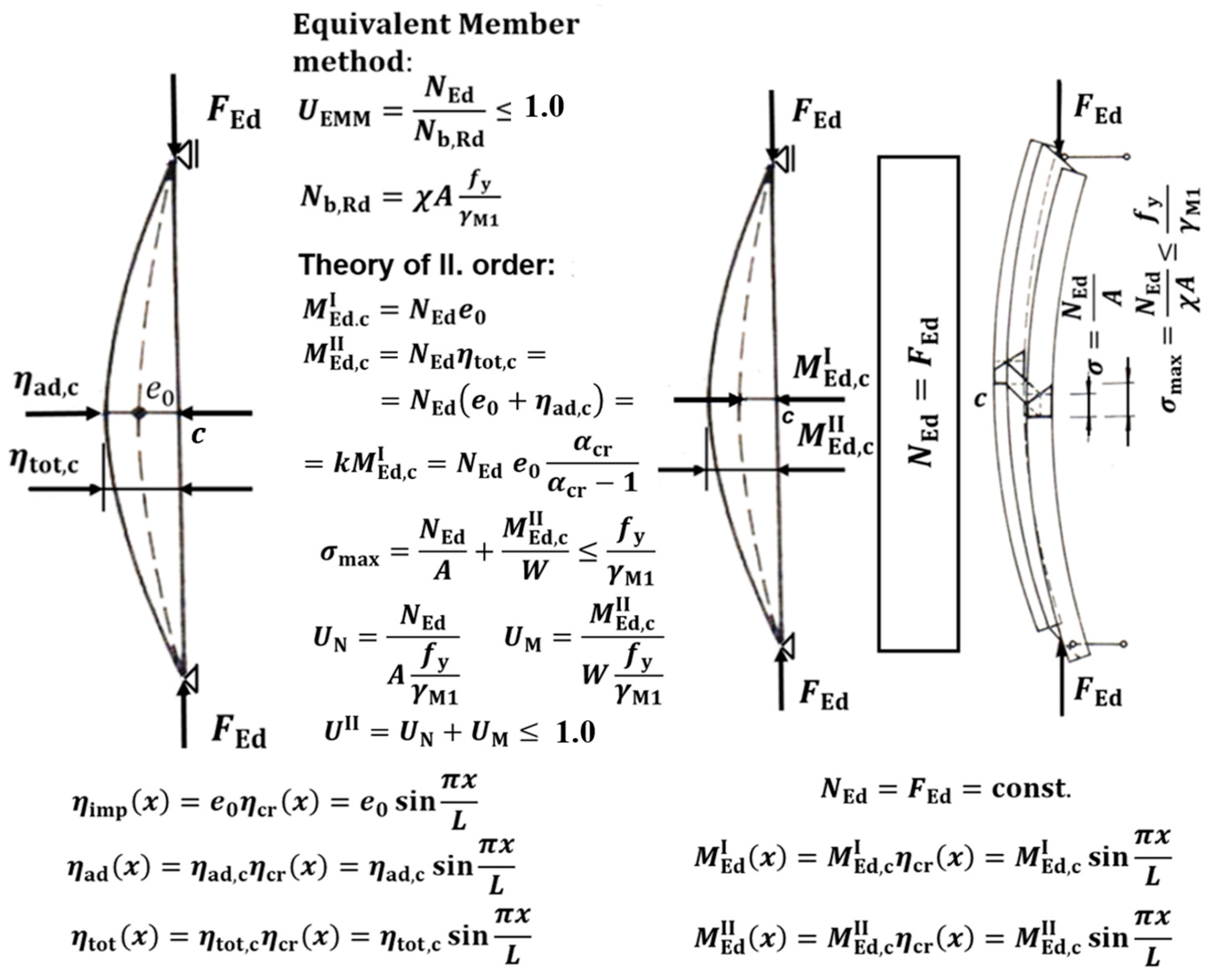
2. Equivalent Member Method

The derivation of the reduction factor χ for the relevant buckling curve: The basic formula for the flexural buckling curve to determine the characteristic resistance of a member under compression reads as so:

$$\sigma =\frac{N_{\mathrm{Ed}}}{A}+\frac{M_{\mathrm{Ed}}^{\mathrm{II}}}{W}=f_y.$$

(1)

After using the characteristic values of cross-section resistances:

$$N_{\mathrm{c},\mathrm{Rk}}=A{f}_{\mathrm{y}}, M_{\mathrm{c},\mathrm{Rk}}=W{f}_{\mathrm{y}},$$

(2)

then Equation (1) may be rewritten as follows:

$$\frac{N_{\mathrm{Ed}}}{N_{\mathrm{c},\mathrm{Rk}}}+\frac{M_{\mathrm{Ed}}^{\mathrm{II}}}{M_{\mathrm{c},\mathrm{Rk}}}=1.0.$$

(3)

The factor by which the design value of the loading would have to be increased to cause elastic instability is as follows:

$${\alpha }_{\mathrm{cr}}=\frac{N_{\mathrm{cr}}}{N_{\mathrm{Ed}}}.$$

(4)

The amplification factor after taking into account second-order effects is as follows:

$$k=\frac{1}{1-\frac{N_{\mathrm{Ed}}}{N_{\mathrm{cr}}}}=\frac{1}{1-\frac{1}{{\alpha }_{\mathrm{cr}}}}=\frac{{\alpha }_{\mathrm{cr}}}{{\alpha }_{\mathrm{cr}}-1}.$$

(5)

The bending moment at the member midspan according to the first-order theory is as follows:

$$M_{\mathrm{Ed}}^{\mathrm{I}}=N_{\mathrm{Ed}}{e}_{0,\mathrm{k}}=N_{\mathrm{Ed}}\alpha \left(\overline{\lambda }-{\overline{\lambda }}_0\right) \frac{W}{A}.$$

(6)

The bending moment at the member midspan according to the second-order theory is as follows:

$$M_{\mathrm{Ed}}^{\mathrm{II}}=k{M}_{\mathrm{Ed}}^{\mathrm{I}}=\frac{1}{1-\frac{N_{\mathrm{Ed}}}{N_{\mathrm{cr}}}}{N}_{\mathrm{Ed}}{e}_{0,\mathrm{k}}=\frac{1}{1-\frac{N_{\mathrm{Ed}}}{N_{\mathrm{cr}}}}{N}_{\mathrm{Ed}}\alpha \left(\overline{\lambda }-{\overline{\lambda }}_0\right) \frac{W}{A}.$$

(7)

The characteristic imperfection amplitude value is as follows:

$$e_{0,\mathrm{k}}=\alpha \left(\overline{\lambda }-{\overline{\lambda }}_0\right) \frac{M_{\mathrm{c},\mathrm{Rk}}}{N_{\mathrm{c},\mathrm{Rk}}}=\alpha \left(\overline{\lambda }-{\overline{\lambda }}_0\right) \frac{W}{A} .$$

(8)

The shape of the equivalent geometrical initial imperfection ${\eta }_{\mathrm{init}}\left(x\right)$ is that of the structure’s elastic critical buckling mode ${\eta }_{\mathrm{cr}}\left(x\right)$. For the investigated member, it comes in the form of a sinus half-wave and includes both structural and geometrical imperfections, as shown by the following:

$${\eta }_{\mathrm{init}}\left(x\right)=e_{0,\mathrm{k}}{\eta }_{\mathrm{cr}}\left(x\right)=e_{0,\mathrm{k}}\sin \left(\frac{\pi x}{L}\right).$$

(9)

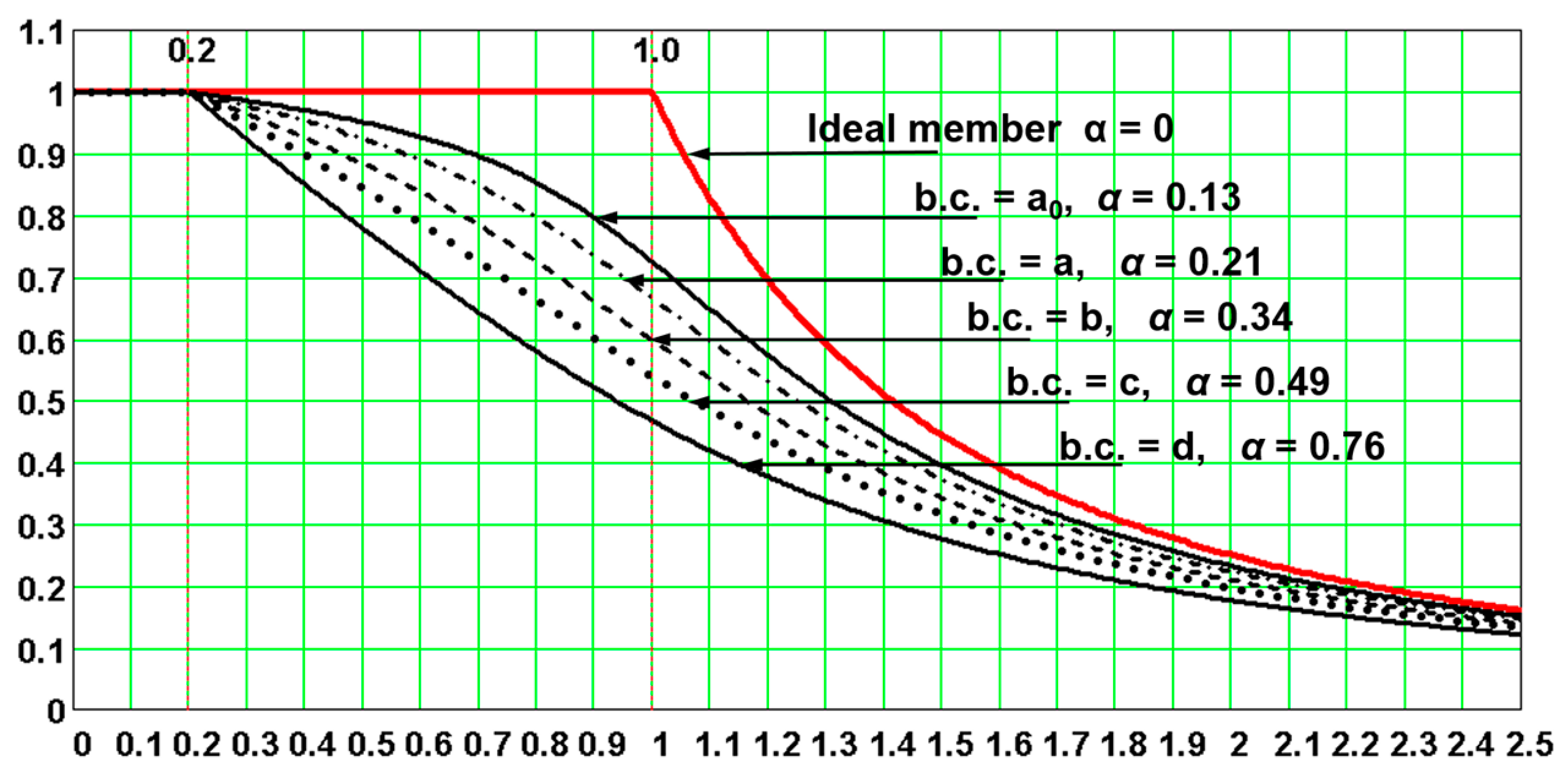
The imperfection factors $\alpha$ corresponding to the appropriate buckling curves are shown in

Table 1. Values of imperfection factors $\alpha$ for ideal member and buckling curves.

Imperfection Factor$\mathit{\alpha }$	For Ideal Member	For Buckling Curves (b.c.s)
		${\mathit{a}}_{\mathbf{0}}$	$\mathit{a}$	$\mathit{b}$	$\mathit{c}$	$\mathit{d}$
	$0$	$0.13$	$0.21$	$0.34$	$0.49$	$0.76$

, together with $\alpha =0$, which is valid for the ideal member.

The relative slenderness $\overline{\lambda }$ and plateau length ${\overline{\lambda }}_0$ of buckling curves are shown in Equation (10). In the steel Eurocode, ${\overline{\lambda }}_0=0.2$. Different ${\overline{\lambda }}_0$ values are used in the aluminium Eurocode.

$$\overline{\lambda }=\sqrt{\frac{N_{\mathrm{c},\mathrm{Rk}}}{N_{\mathrm{cr}}} }, {\overline{\lambda }}_0=0.2.$$

(10)

After inserting the reduction factor χ (11) and fraction (12) from Equation (3), the following was obtained:

$$\frac{N_{\mathrm{Ed}}}{N_{\mathrm{c},\mathrm{Rk}}}= \chi ,$$

(11)

$$\frac{M_{\mathrm{Ed}}^{\mathrm{II}}}{M_{\mathrm{c},\mathrm{Rk}}}=\frac{k{N}_{\mathrm{Ed}}{e}_{0,\mathrm{k}}}{W{f}_{\mathrm{y}}}= \frac{1}{1-\frac{N_{\mathrm{Ed}}}{N_{\mathrm{cr}}}}\frac{N_{\mathrm{Ed}}\alpha \left(\overline{\lambda }-{\overline{\lambda }}_0\right) \frac{W}{A}}{W{f}_{\mathrm{y}}}= \frac{1}{1-\frac{N_{\mathrm{Ed}}}{N_{\mathrm{c},\mathrm{Rk}}}\frac{N_{\mathrm{c},\mathrm{Rk}}}{N_{\mathrm{cr}}}}\frac{N_{\mathrm{Ed}}\alpha \left(\overline{\lambda }-{\overline{\lambda }}_0\right) }{N_{\mathrm{c},\mathrm{Rk}}}=\frac{\chi \alpha \left(\overline{\lambda }-{\overline{\lambda }}_0\right)}{1-\chi {\overline{\lambda }}^2}.$$

(12)

The basic quadratic Equation (13) was obtained for reduction factor χ:

$$\chi +\frac{\alpha \left(\overline{\lambda }-{\overline{\lambda }}_0\right)}{1-\chi {\overline{\lambda }}^2}\chi =1.0,$$

(13)

which may be rewritten in the following way:

$${\overline{\lambda }}^2{\chi }^2-\left[1+\alpha \left(\overline{\lambda }-{\overline{\lambda }}_0\right)+{\overline{\lambda }}^2\right]\chi +1.0=0.$$

(14)

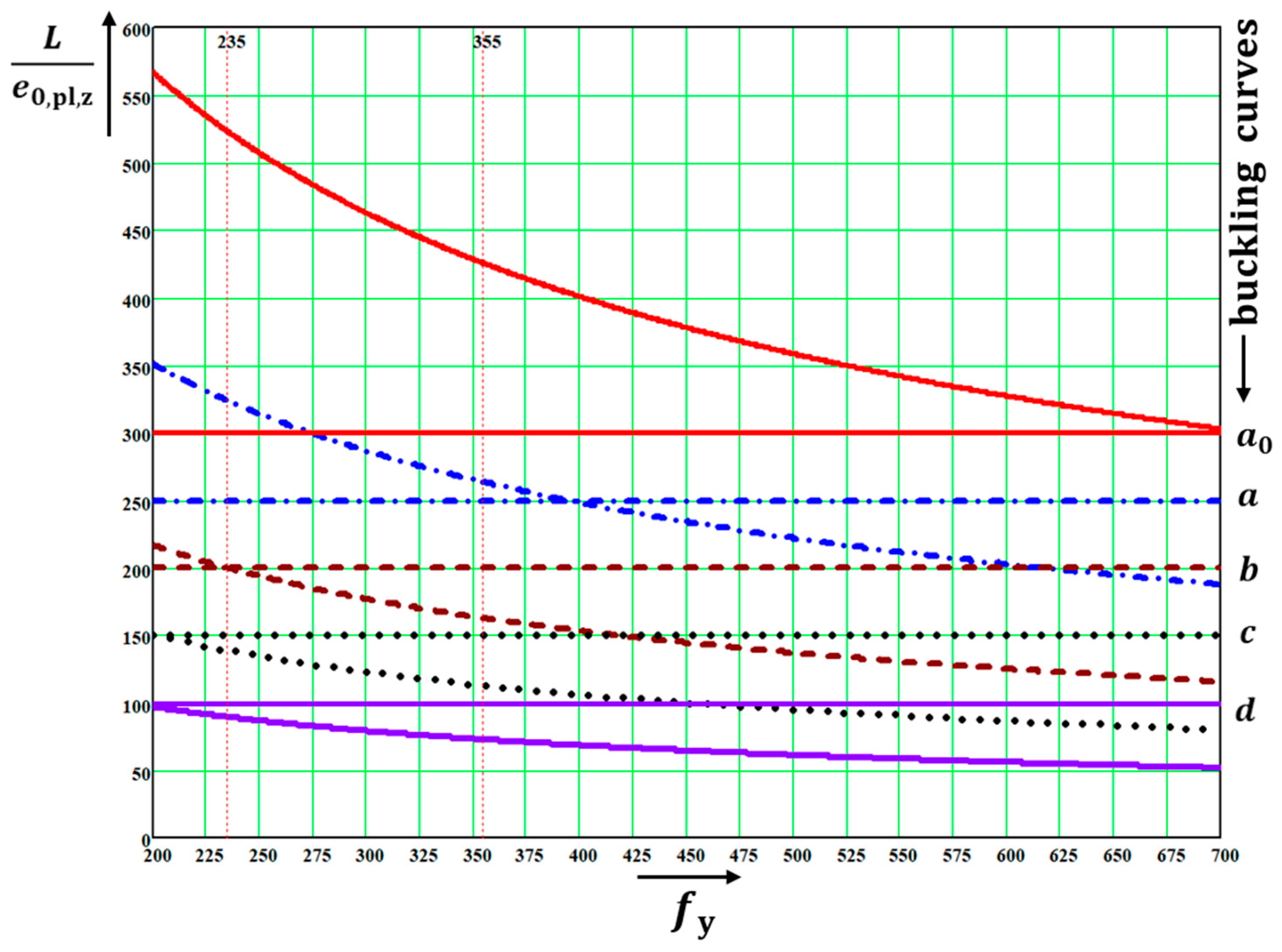
The solution of quadratic Equation (14) leads to “European column buckling curves” (Figure 1).

$$\chi \left(\alpha ,\overline{\lambda },{\overline{\lambda }}_0=0.2\right)= \frac{1}{0.5 \left[1+\alpha \left(\overline{\lambda }-{\overline{\lambda }}_0\right)+{\overline{\lambda }}^2 \right]+\sqrt{{\left\{0.5 \left[1+\alpha \left(\overline{\lambda }-{\overline{\lambda }}_0\right)+{\overline{\lambda }}^2 \right]\right\}}^2-{\overline{\lambda }}^2}}=\frac{1}{\Phi +\sqrt{{\Phi }^2-{\overline{\lambda }}^2}}.$$

(15)

A compression member should be verified against buckling as follows:

$$N_{\mathrm{Ed}}\le N_{\mathrm{b},\mathrm{Rd}}=\frac{\chi A{f}_{\mathrm{y}}}{{\gamma }_{\mathrm{M}1}}.$$

(16)

Equation (15) may be written in this way by showing the utilization factor $U$ value:

$$U=\frac{N_{\mathrm{Ed}}}{N_{\mathrm{b},\mathrm{Rd}}}\le 1.0.$$

(17)

The maximum design value of the compression force $N_{\mathrm{Ed}}$ equals the design buckling resistance of the compression member $N_{\mathrm{b},\mathrm{Rd}}$ when the utilization factor $U=1.0$:

$$N_{\mathrm{Ed},\max }=N_{\mathrm{b},\mathrm{Rd}}=\frac{\chi A{f}_{\mathrm{y}}}{{\gamma }_{\mathrm{M}1}}.$$

(18)

The same results for $N_{\mathrm{Ed}}=N_{\mathrm{b},\mathrm{Rd}}$ can be obtained when the second-order theory is used under the condition that the characteristic value of the imperfection amplitude $e_{0,\mathrm{k}}$ is replaced with the design value of the imperfection amplitude $e_{0,\mathrm{d}}$:

$$e_{0,\mathrm{d}}=\alpha \left(\overline{\lambda }-{\overline{\lambda }}_0\right)\frac{1-\frac{\chi {\overline{\lambda }}^2}{{\gamma }_{\mathrm{M}1}}}{1-\chi {\overline{\lambda }}^2} \frac{W}{A}.$$

(19)

The relative design value of the imperfection amplitude is as follows:

$$\frac{e_{0,\mathrm{d}}}{j}=\alpha \left(\overline{\lambda }-{\overline{\lambda }}_0\right)\frac{1-\frac{\chi {\overline{\lambda }}^2}{{\gamma }_{\mathrm{M}1}}}{1-\chi {\overline{\lambda }}^2},$$

(20)

where:

$$j=\frac{W}{A}.$$

(21)

The following equations are valid for the maximum design value of the compression force $N_{\mathrm{Ed}}=N_{\mathrm{b},\mathrm{Rd}}$ when the utilization factor $U=1.0$:

$$N_{\mathrm{Ed}}=N_{\mathrm{b},\mathrm{Rd}}=\frac{\chi A{f}_{\mathrm{y}}}{{\gamma }_{\mathrm{M}1}}.$$

(22)

Consequently, the following were similarly obtained as above:

$${\alpha }_{\mathrm{cr}}=\frac{N_{\mathrm{cr}}}{N_{\mathrm{Ed}}}=\frac{{\gamma }_{\mathrm{M}1}}{\chi {\overline{\lambda }}^2},$$

(23)

$$k=\frac{1}{1-\frac{1}{{\alpha }_{\mathrm{cr}}}}=\frac{{\alpha }_{\mathrm{cr}}}{{\alpha }_{\mathrm{cr}}-1}=\frac{{\gamma }_{\mathrm{M}1}}{{\gamma }_{\mathrm{M}1}-\chi {\overline{\lambda }}^2},$$

(24)

$$M_{\mathrm{Ed}}^{\mathrm{I}}=N_{\mathrm{Ed}}{e}_{0,\mathrm{d}}=N_{\mathrm{Ed}}\alpha \left(\overline{\lambda }-{\overline{\lambda }}_0\right)\frac{1-\frac{\chi {\overline{\lambda }}^2}{{\gamma }_{\mathrm{M}1}}}{1-\chi {\overline{\lambda }}^2} \frac{W}{A},$$

(25)

$$M_{\mathrm{Ed}}^{\mathrm{II}}=k{M}_{\mathrm{Ed}}^{\mathrm{I}}=\frac{1}{1-\frac{1}{{\alpha }_{\mathrm{cr}}}}{N}_{\mathrm{Ed}}{e}_{0,\mathrm{d}}=\frac{{\gamma }_{\mathrm{M}1}}{{\gamma }_{\mathrm{M}1}-\chi {\overline{\lambda }}^2}{N}_{\mathrm{c},\mathrm{Rd}}\alpha \left(\overline{\lambda }-{\overline{\lambda }}_0\right)\frac{1-\frac{\chi {\overline{\lambda }}^2}{{\gamma }_{\mathrm{M}1}}}{1-\chi {\overline{\lambda }}^2} \frac{W}{A}=\frac{\alpha \left(\overline{\lambda }-{\overline{\lambda }}_0\right)}{1-\chi {\overline{\lambda }}^2}\chi W\frac{f_{\mathrm{y}}}{{\gamma }_{\mathrm{M}1}}.$$

(26)

The design value of the amplitude ${\eta }_{\mathrm{ad},\mathrm{d},\mathrm{c}}$ of the additional deformation ${\eta }_{\mathrm{add}}\left(x\right)$ caused by the force $N_{\mathrm{Ed}}$ on the member with the equivalent geometrical initial imperfection ${\eta }_{\mathrm{init}}\left(x\right)$ is as follows:

$${\eta }_{\mathrm{ad},\mathrm{d},\mathrm{c}}= \frac{1}{{\alpha }_{\mathrm{cr}}-1}{e}_{0,\mathrm{d}}=\frac{\alpha \left(\overline{\lambda }-{\overline{\lambda }}_0\right)\chi {\overline{\lambda }}^2}{\left(1-\chi {\overline{\lambda }}^2\right){\gamma }_{\mathrm{M}1}}\frac{W}{A}.$$

(27)

The relative design amplitude ${\eta }_{\mathrm{ad},\mathrm{d},\mathrm{c}}/j$ of the additional deformation ${\eta }_{\mathrm{ad},\mathrm{d}}\left(x\right)$ is as follows:

$$\frac{{\eta }_{\mathrm{ad},\mathrm{d},\mathrm{c}}}{j}=\frac{1}{{\alpha }_{\mathrm{cr}}-1}\frac{e_{0,\mathrm{d}}}{j}=\frac{\alpha \left(\overline{\lambda }-{\overline{\lambda }}_0\right)\chi {\overline{\lambda }}^2}{\left(1-\chi {\overline{\lambda }}^2\right){\gamma }_{\mathrm{M}1}}.$$

(28)

The amplitude ${\eta }_{\mathrm{tot},\mathrm{c}}$ of the total deformation ${\eta }_{\mathrm{tot}}\left(x\right)$ is as follows:

$${\eta }_{\mathrm{tot},\mathrm{c}}=e_{0,\mathrm{d}}+{\eta }_{\mathrm{ad},\mathrm{d},\mathrm{c}}=k{e}_{0,\mathrm{d}}=\frac{{\alpha }_{\mathrm{cr}}}{{\alpha }_{\mathrm{cr}}-1}{e}_{0,\mathrm{d}}={\alpha }_{\mathrm{cr}}{\eta }_{\mathrm{ad},\mathrm{d},\mathrm{c}}=\frac{\alpha \left(\overline{\lambda }-{\overline{\lambda }}_0\right)}{1-\chi {\overline{\lambda }}^2} \frac{W}{A}.$$

(29)

The relative amplitude ${\eta }_{\mathrm{tot},\mathrm{c}}/j$ of the total deformation ${\eta }_{\mathrm{tot}}\left(x\right)$ is as follows:

$$\frac{{\eta }_{\mathrm{tot},\mathrm{c}}}{j}=\frac{e_{0,\mathrm{d}}+{\eta }_{\mathrm{ad},\mathrm{d},\mathrm{c}}}{j}=k\frac{e_{0,\mathrm{d}}}{j}=\frac{{\alpha }_{\mathrm{cr}}}{{\alpha }_{\mathrm{cr}}-1}\frac{e_{0,\mathrm{d}}}{j}={\alpha }_{\mathrm{cr}}\frac{{\eta }_{\mathrm{ad},\mathrm{d},\mathrm{c}}}{j}=\frac{\alpha \left(\overline{\lambda }-{\overline{\lambda }}_0\right)}{1-\chi {\overline{\lambda }}^2}.$$

(30)

The partial utility factors are:

$$U_{\mathrm{N}}=\chi , U_{\mathrm{M}}=\frac{\alpha \left(\overline{\lambda }-{\overline{\lambda }}_0\right)}{1-\chi {\overline{\lambda }}^2} \chi .$$

(31)

The utility factor is as follows:

$$U^{\mathrm{II}}=U_{\mathrm{N}}+U_{\mathrm{M}}=\left[1+\frac{\alpha \left(\overline{\lambda }-{\overline{\lambda }}_0\right)}{1-\chi {\overline{\lambda }}^2}\right]\chi .$$

(32)

Evidence for the utility factor $U$, as defined by Equation (32), equaling 1.0 may be obtained after inserting the relative slenderness $\overline{\lambda }$ (Equation (10)) and reduction factor $\chi$ (Equation (13)) in Equation (32) and arranging it. This may be achieved, e.g., by the MATHCAD commands Symbolics and Simplify.

Removing safety factor ${\gamma }_{\mathrm{M}1}$ from amplitude $e_{0,\mathrm{d}}$ leads to its value being $1.00÷2.19$ times lower (

Table 2. Removing safety factor ${\gamma }_{\mathrm{M}1}$ from amplitude $e_{0,\mathrm{d}}$ decreases its value depending on imperfection factor $\alpha$ and relative slenderness $\overline{\lambda }$.

$\frac{{\mathit{e}}_{0,\mathbf{d}}}{{\mathit{e}}_{0,\mathbf{k}}}=\frac{1-\frac{\mathit{\chi }{\overline{\mathit{\lambda }}}^2}{{\mathit{\gamma }}_{\mathbf{M}1}}}{1-\mathit{\chi }{\overline{\mathit{\lambda }}}^2}$		$\overline{\mathit{\lambda }}$
		$0.2$	$0.8$	$1.0$	$1.5$	$2.0$
$\mathbf{\alpha }$	$0.13$	$1.004$	$1.109$	$1.24$	$1.732$	$2.193$
	$0.21$	$1.004$	$1.094$	$1.181$	$1.47$	$1.748$
	$0.34$	$1.004$	$1.079$	$1.135$	$1.304$	$1.47$
	$0.49$	$1.004$	$1.067$	$1.107$	$1.22$	$1.331$
	$0.76$	$1.004$	$1.054$	$1.08$	$1.15$	$1.219$

).

2.1. Numerical Example 1

Comparison of the verifications according to Equivalent Member method and second-order theory is illustrated in Figure 2.

$$\begin{array}{c}\mathrm{Input} \mathrm{values}: \mathrm{steel} \mathrm{S}235 f_{\mathrm{y}}=235 \mathrm{MPa}, {\gamma }_{\mathrm{M}1}=1,1, E=210,000 \mathrm{MPa}.\\ \mathrm{IPE} 500: h=500 \mathrm{mm}, b=200 \mathrm{mm}, t_{\mathrm{f}}=16 \mathrm{mm}, t_{\mathrm{w}}=10.2 \mathrm{mm}, r=21 \mathrm{mm},\\ A=115.52{ \mathrm{cm}}^2, I_{\mathrm{y}}=48,199{ \mathrm{cm}}^4, W_{\mathrm{el},\mathrm{y}}=1928{ \mathrm{cm}}^3, W_{\mathrm{pl},\mathrm{y}}=2194{ \mathrm{cm}}^3, i_{\mathrm{y}}=20.43 \mathrm{cm},\\ j_{\mathrm{y}}=\frac{W_{\mathrm{el},\mathrm{y}}}{A}=16.7 \mathrm{cm}, I_{\mathrm{z}}=2142{ \mathrm{cm}}^4, W_{\mathrm{el},\mathrm{z}}=214.2{ \mathrm{cm}}^3, W_{\mathrm{pl},\mathrm{z}}=335.87{ \mathrm{cm}}^3, i_{\mathrm{z}}=\\ 4.306 \mathrm{cm},j_{\mathrm{z}}=\frac{W_{\mathrm{el},\mathrm{z}}}{A}=1.9 \mathrm{cm}, L=12 \mathrm{m}, {\beta }_y=1.0, {\beta }_{\mathrm{z}}=0.5, L_{\mathrm{cr},\mathrm{y}}={\beta }_{y}L=12 \mathrm{m}, L_{\mathrm{cr},\mathrm{z}}={\beta }_{\mathrm{z}}L=6 \mathrm{m}. \end{array}$$

(a) Verification against the flexural buckling perpendicular to the strong axis y–y.

For the force $N_{\mathrm{Ed}}$, the EM method gives:

$$N_{\mathrm{Ed}}=N_{\mathrm{b},\mathrm{Rd}}=\frac{\chi A{f}_{\mathrm{y}}}{{\gamma }_{\mathrm{M}1}}=\frac{0.88 · 115.52{ \mathrm{cm}}^2 · 235 \mathrm{MPa}}{1.1}=2171.883 \mathrm{kN}, U_{\mathrm{EMM}}=\frac{N_{\mathrm{Ed}}}{N_{\mathrm{b},\mathrm{Rd}}}=1.0.$$

(33)

The results of the second-order theory are summarized in

Table 3. Results of the second-order theory for flexural buckling perpendicular to strong axis y–y.

${\mathit{L}}_{\mathit{c}\mathit{r}}$ (m)	$\overline{\mathit{\lambda }}$	${\overline{\mathit{\lambda }}}_0$	$\mathit{\alpha }$	$\mathit{\Phi }$	$\mathit{\chi }$	$\frac{{\mathit{e}}_{0,\mathbf{k}}}{\mathit{j}}$	${\mathit{e}}_{0,\mathbf{k}}$ (mm)	$\frac{{\mathit{e}}_{0,\mathbf{d}}}{\mathit{j}}\ast$	${\mathit{e}}_{0,\mathbf{d}}\ast$ (mm)
$12$	$0.626$	$0.2$	$0.21$	$0.74$	$0.88$	$0.0894$	$14.9$	$0.0936$	$15.63$
$\frac{{\eta }_{\mathrm{ad},\mathrm{d},\mathrm{c}}}{j}\ast$	${\eta }_{\mathrm{ad},\mathrm{d},\mathrm{c}}\ast$ $(\mathrm{mm}$)	$\frac{{\eta }_{\mathrm{tot},\mathrm{c}}}{j}$	${\eta }_{\mathrm{tot},\mathrm{c}}$ $\left(\mathrm{mm}\right)$	${\alpha }_{\mathrm{cr}}\ast$	$k\ast$	$M_{\mathrm{c}}^{\mathrm{I}}\ast$ $\left(\mathrm{kNm}\right)$	$M_{\mathrm{c}}^{\mathrm{II}}\ast$ $\left(\mathrm{kNm}\right)$	$U_{\mathrm{N}}$	$U_{\mathrm{M}}$
$0.0427$	$7.12$	$0.1363$	$22.75$	$3.194$	$1.456$	$33.941$	$49.409$	$0.88$	$0.12$

Note: symbol $\ast$ indicates that the values of these quantities also depend on safety factor ${\gamma }_{\mathrm{M}1}$.

.

$$U^{\mathrm{II}}=U_{\mathrm{N}}+U_{\mathrm{M}}=0.88+0.12=1.0.$$

(34)

If the calculation in Equation (34) is repeated according to the second-order theory with $e_{0,\mathrm{k}}$ instead of $e_{0,\mathrm{d}}$ (that is, when ${\gamma }_{\mathrm{M}1}$ is removed from $e_{0,\mathrm{d}}),$ the following results are obtained:

$${\eta }_{\mathrm{ad},\mathrm{d},\mathrm{c},e_{0,\mathrm{k}}}=\frac{\alpha \left(\overline{\lambda }-{\overline{\lambda }}_0\right)\chi {\overline{\lambda }}^2}{{\gamma }_{\mathrm{M}1}-\chi {\overline{\lambda }}^2}\frac{W}{A}=6.798 \mathrm{mm},$$

(35)

$${\eta }_{\mathrm{tot},\mathrm{c},e_{0,\mathrm{k}}}=e_{0,\mathrm{k}}+{\eta }_{\mathrm{ad},\mathrm{d},\mathrm{c},e_{0,\mathrm{k}},}=k{e}_{0,\mathrm{k}}={\alpha }_{\mathrm{cr}}{\eta }_{\mathrm{ad},\mathrm{d},\mathrm{c},e_{0,\mathrm{k}}}=\frac{\alpha \left(\overline{\lambda }-{\overline{\lambda }}_0\right){\gamma }_{\mathrm{M}1}}{{\gamma }_{\mathrm{M}1}-\chi {\overline{\lambda }}^2}\frac{W}{A}=21.71 \mathrm{mm},$$

(36)

$$U_{\mathrm{N}}=\chi =0.88, U_{\mathrm{M},e_{0,\mathrm{k}}}=\frac{\alpha \left(\overline{\lambda }-{\overline{\lambda }}_0\right){\gamma }_{\mathrm{M}1}}{{\gamma }_{\mathrm{M}1}-\chi {\overline{\lambda }}^2} \chi =0.114,$$

(37)

$$U_{e_{0,\mathrm{k}}}^{\mathrm{II}}=U_{\mathrm{N}}+U_{\mathrm{M},e_{0,\mathrm{k}}}=\left[1+\frac{\alpha \left(\overline{\lambda }-{\overline{\lambda }}_0\right){\gamma }_{\mathrm{M}1}}{{\gamma }_{\mathrm{M}1}-\chi {\overline{\lambda }}^2}\right]\chi =0.88+0.114=0.995.$$

(38)

In this case, removing the safety factor ${\gamma }_{\mathrm{M}1}$ from the amplitude $e_{0,\mathrm{d}}$ leads to an incorrect value of the utility factor $U^{\mathrm{II}},$ which is calculated by the second-order theory, where 0.5% is on the unsafe side.

(b) Verification against flexural buckling perpendicular to the weak axis z–z.

For the force $N_{\mathrm{Ed}}$, the EM method gives:

$$N_{\mathrm{Ed}}=N_{\mathrm{b},\mathrm{Rd}}=\frac{\chi A{f}_{\mathrm{y}}}{1.1}=\frac{0.348 · 115.52{ \mathrm{cm}}^2 · 235 \mathrm{MPa}}{1.1}=859.584 \mathrm{kN}, U_{\mathrm{EMM}}=\frac{N_{\mathrm{Ed}}}{N_{\mathrm{b},\mathrm{Rd}}}=1.0.$$

(39)

The results of the second-order theory are summarized in

Table 4. Results of the second-order theory for flexural buckling perpendicular to weak axis z–z.

${\mathit{L}}_{\mathit{c}\mathit{r}}$ (m)	$\overline{\mathit{\lambda }}$	${\overline{\mathit{\lambda }}}_0$	$\mathit{\alpha }$	$\mathit{\Phi }$	$\mathit{\chi }$	$\frac{{\mathit{e}}_{0,\mathbf{k}}}{\mathit{j}}$	${\mathit{e}}_{0,\mathbf{k}}$ (mm)	$\frac{{\mathit{e}}_{0,\mathbf{d}}}{\mathit{j}}\ast$	${\mathit{e}}_{0,\mathbf{d}}\ast$ (mm)
$6$	$1.484$	$0.2$	$0.34$	$1.819$	$0.348$	$0.436$	$8.09$	$0.567$	$10.51$
$\frac{{\eta }_{\mathrm{ad},\mathrm{d},\mathrm{c}}}{j}\ast$	${\eta }_{\mathrm{ad},\mathrm{d},\mathrm{c}}\ast$ (mm)	$\frac{{\eta }_{\mathrm{tot},\mathrm{c}}}{j}$	${\eta }_{\mathrm{tot},\mathrm{c}}$ $\left(\mathrm{mm}\right)$	${\alpha }_{\mathrm{cr}}\ast$	$k\ast$	$M_{\mathrm{c}}^{\mathrm{I}}\ast$ $\left(\mathrm{kNm}\right)$	$M_{\mathrm{c}}^{\mathrm{II}}\ast$ $\left(\mathrm{kNm}\right)$	$U_{\mathrm{N}}$	$U_{\mathrm{M}}$
$1.304$	$24.18$	$1.871$	$34.69$	$1.435$	$3.301$	$9.035$	$29.822$	$0.348$	$0.652$

Note: symbol $\ast$ indicates that the values of these quantities also depend on safety factor ${\gamma }_{\mathrm{M}1}$.

.

$$U^{\mathrm{II}}=U_{\mathrm{N}}+U_{\mathrm{M}}=0.348+0.652=1.0.$$

(40)

If, according to the second-order theory, the calculation in Equation (40) is repeated with $e_{0,\mathrm{k}}$ instead of $e_{0,\mathrm{d}}$ (that is, when ${\gamma }_{\mathrm{M}1}$ is removed from $e_{0,\mathrm{d}}),$ the following results are obtained:

$${\eta }_{\mathrm{ad},\mathrm{d},\mathrm{c},e_{0,\mathrm{k}}}=\frac{\alpha \left(\overline{\lambda }-{\overline{\lambda }}_0\right)\chi {\overline{\lambda }}^2}{{\gamma }_{\mathrm{M}1}-\chi {\overline{\lambda }}^2}\frac{W}{A}=18.619 \mathrm{mm},$$

(41)

$${\eta }_{\mathrm{tot},\mathrm{c},e_{0,\mathrm{k}}}=e_{0,\mathrm{k}}+{\eta }_{\mathrm{ad},\mathrm{d},\mathrm{c},e_{0,\mathrm{k}},}=k{e}_{0,\mathrm{k}}={\alpha }_{\mathrm{cr}}{\eta }_{\mathrm{ad},\mathrm{d},\mathrm{c},e_{0,\mathrm{k}}}=\frac{\alpha \left(\overline{\lambda }-{\overline{\lambda }}_0\right){\gamma }_{\mathrm{M}1}}{{\gamma }_{\mathrm{M}1}-\chi {\overline{\lambda }}^2}\frac{W}{A}=26.712 \mathrm{mm},$$

(42)

$$M_{\mathrm{c}}^{\mathrm{II}}=859.584 \mathrm{kN}. 26.712 \mathrm{mm}=22.961 \mathrm{kN},$$

(43)

$$U_{\mathrm{N}}=\chi =0.348, U_{\mathrm{M},e_{0,\mathrm{k}}}=\frac{\alpha \left(\overline{\lambda }-{\overline{\lambda }}_0\right){\gamma }_{\mathrm{M}1}}{{\gamma }_{\mathrm{M}1}-\chi {\overline{\lambda }}^2} \chi =0.502,$$

(44)

$$U_{e_{0,\mathrm{k}}}^{\mathrm{II}}=U_{\mathrm{N}}+U_{\mathrm{M},e_{0,\mathrm{k}}}=\left[1+\frac{\alpha \left(\overline{\lambda }-{\overline{\lambda }}_0\right){\gamma }_{\mathrm{M}1}}{{\gamma }_{\mathrm{M}1}-\chi {\overline{\lambda }}^2}\right]\chi =0.348+0.502=0.85.$$

(45)

In this case, removing the safety factor ${\gamma }_{\mathrm{M}1}$ from the amplitude $e_{0,\mathrm{d}}$ leads to an incorrect value of the utility factor $U^{\mathrm{II}},$ which is calculated by the second-order theory where 15% is on the unsafe side.

The distributions of functions $\chi =U_{\mathrm{N}}, {\alpha }_{\mathrm{cr}}, k, e_{0,\mathrm{d}}/j, {\eta }_{\mathrm{tot},\mathrm{c}}, U_{\mathrm{M}}, U^{\mathrm{II}}=U_{\mathrm{N}}+U_{\mathrm{M}}=1.0$ are drawn in Figure 3, Figure 4, Figure 5, Figure 6, Figure 7, Figure 8, Figure 9, Figure 10, Figure 11, Figure 12 and Figure 13 depending on the safety factor ${\gamma }_{\mathrm{M}1}=1.0 \mathrm{and} 1.1.$ 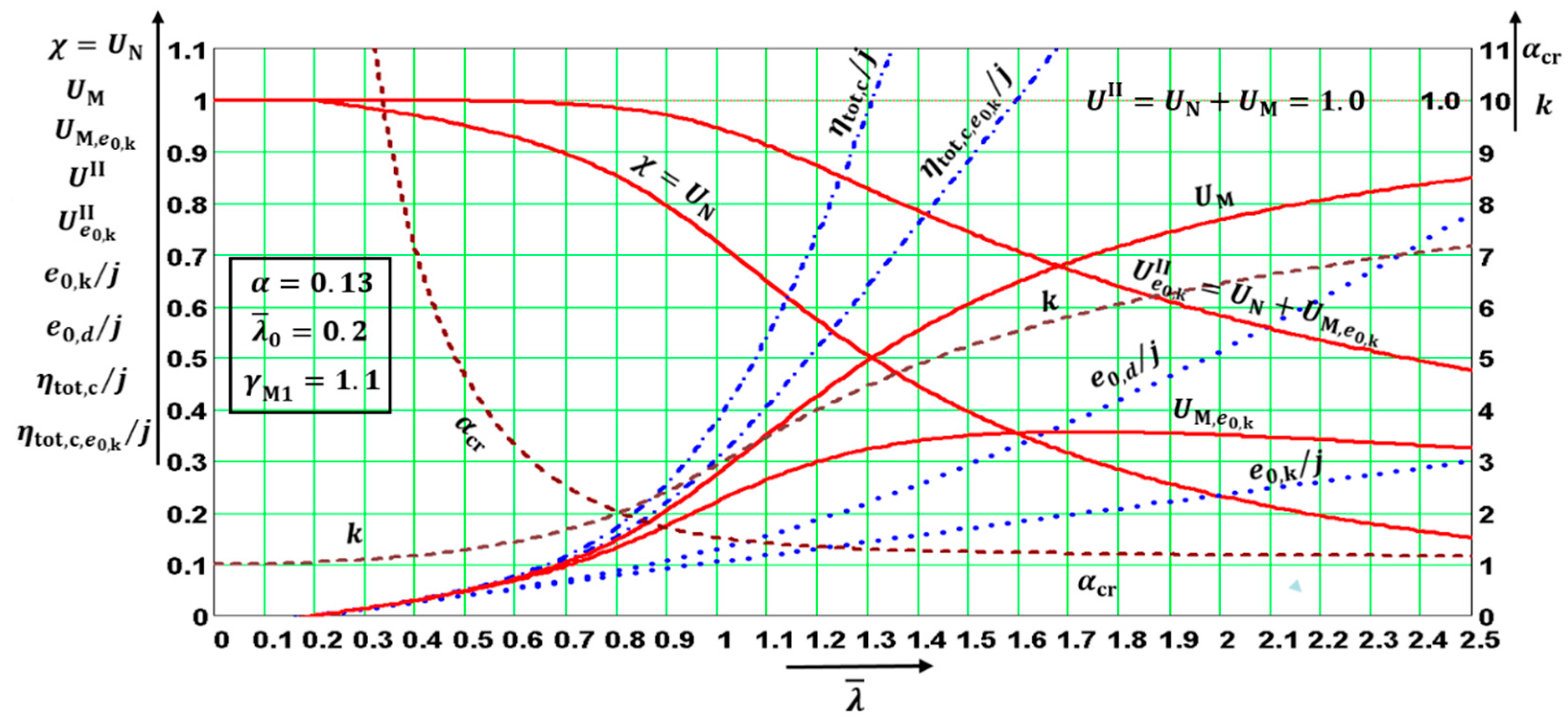In Figure 4 and Figure 13, ${\eta }_{\mathrm{ad},\mathrm{d},\mathrm{c},e_{0,\mathrm{k}}}, {\eta }_{\mathrm{tot},\mathrm{c},e_{0,\mathrm{k}}}, U_{\mathrm{M},e_{0,\mathrm{k}}}, \mathrm{and} U_{e_{0,\mathrm{k}}}^{\mathrm{II}}$ are also drawn, where the differences between the functions $e_{0,\mathrm{d}}/j$ and $e_{0,\mathrm{k}}/j,$ ${\eta }_{\mathrm{tot},\mathrm{c}}$ and ${\eta }_{\mathrm{tot},\mathrm{c},e_{0,\mathrm{k}}},$ $U_{\mathrm{M}}$ and $U_{\mathrm{M},e_{0,\mathrm{k}}}, U^{\mathrm{II}}$ and $U_{e_{0,\mathrm{k}}}^{\mathrm{II}}$ are shown. For the parameters investigated in Figure 4, these differences are the biggest. 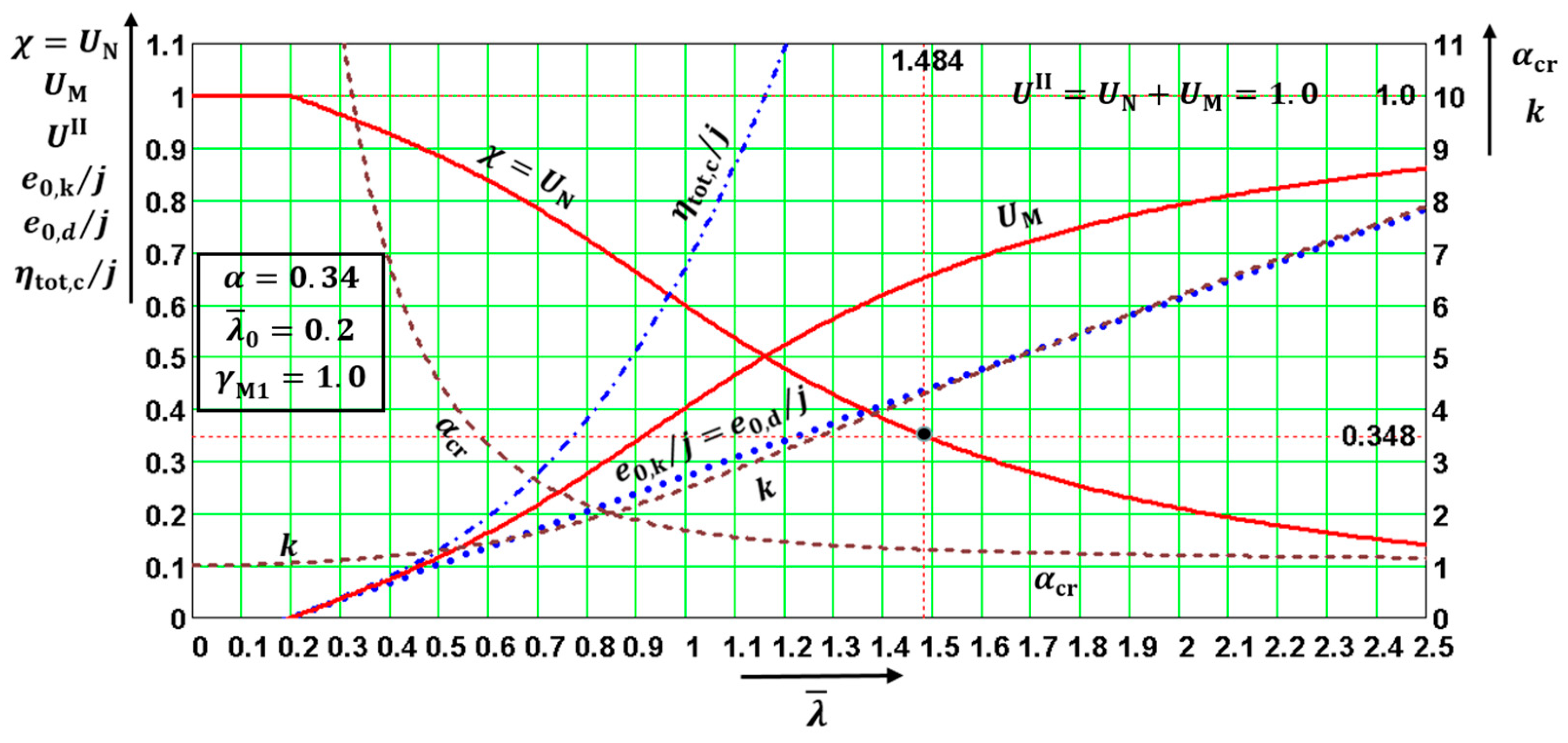Figure 13 also relates to Numerical Example 2, given below.

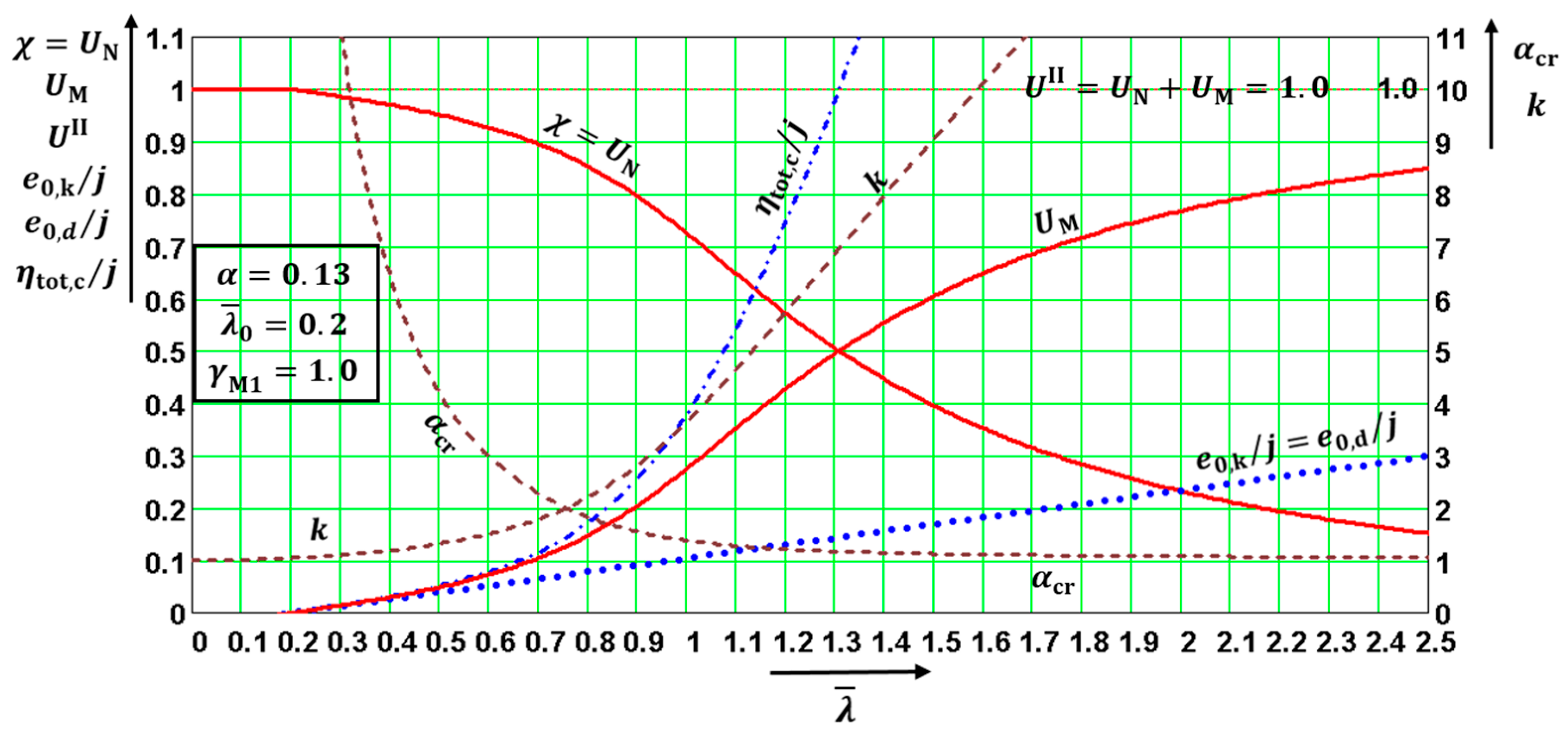
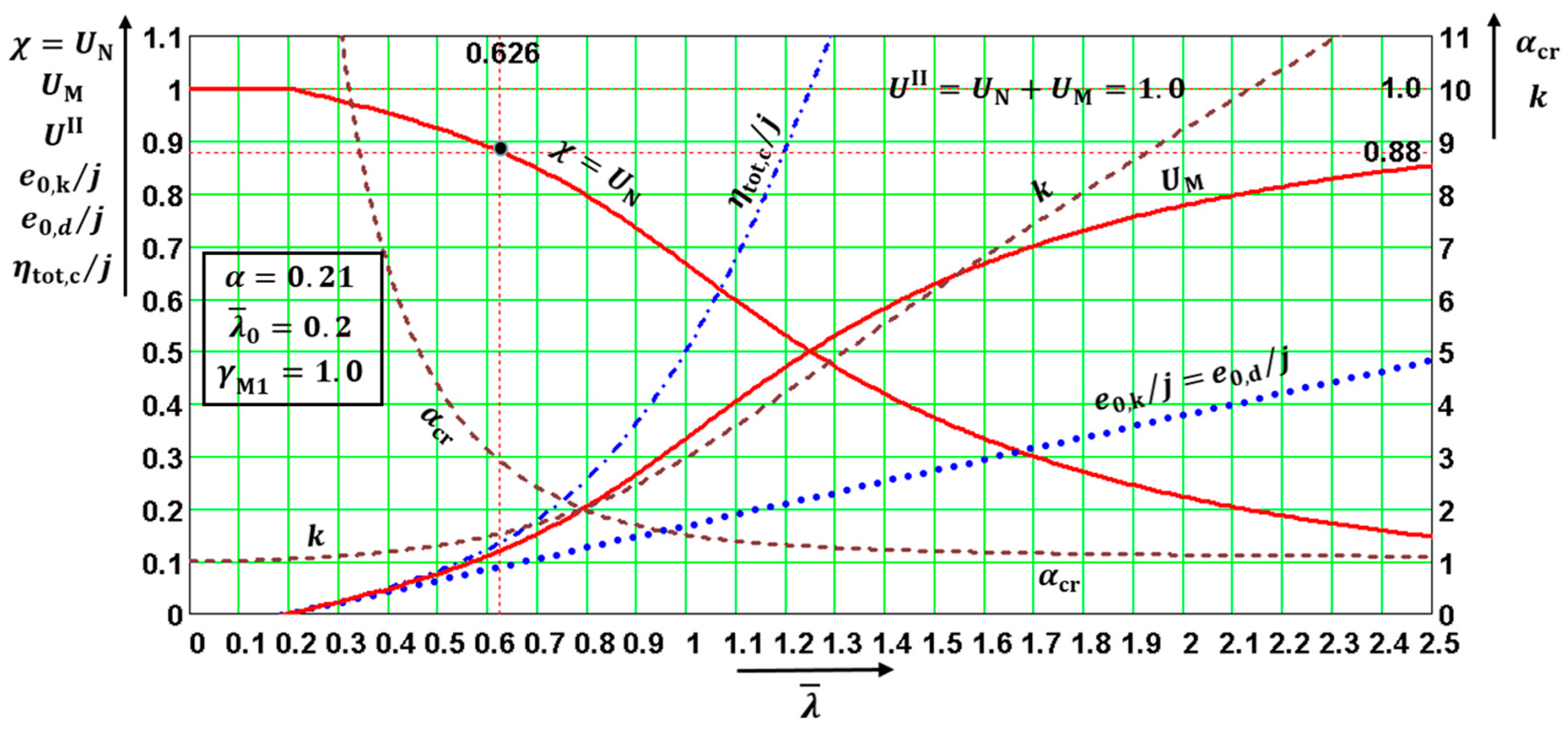
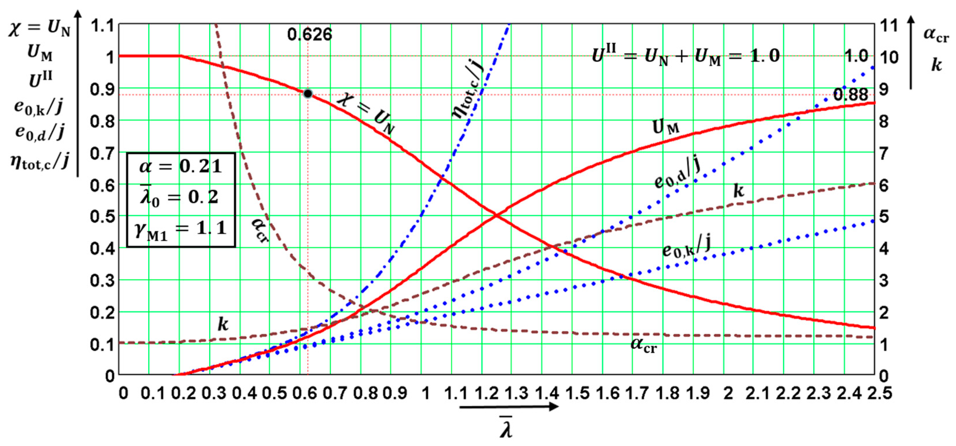
2.2. Geometrical Interpretations of the above Quantities

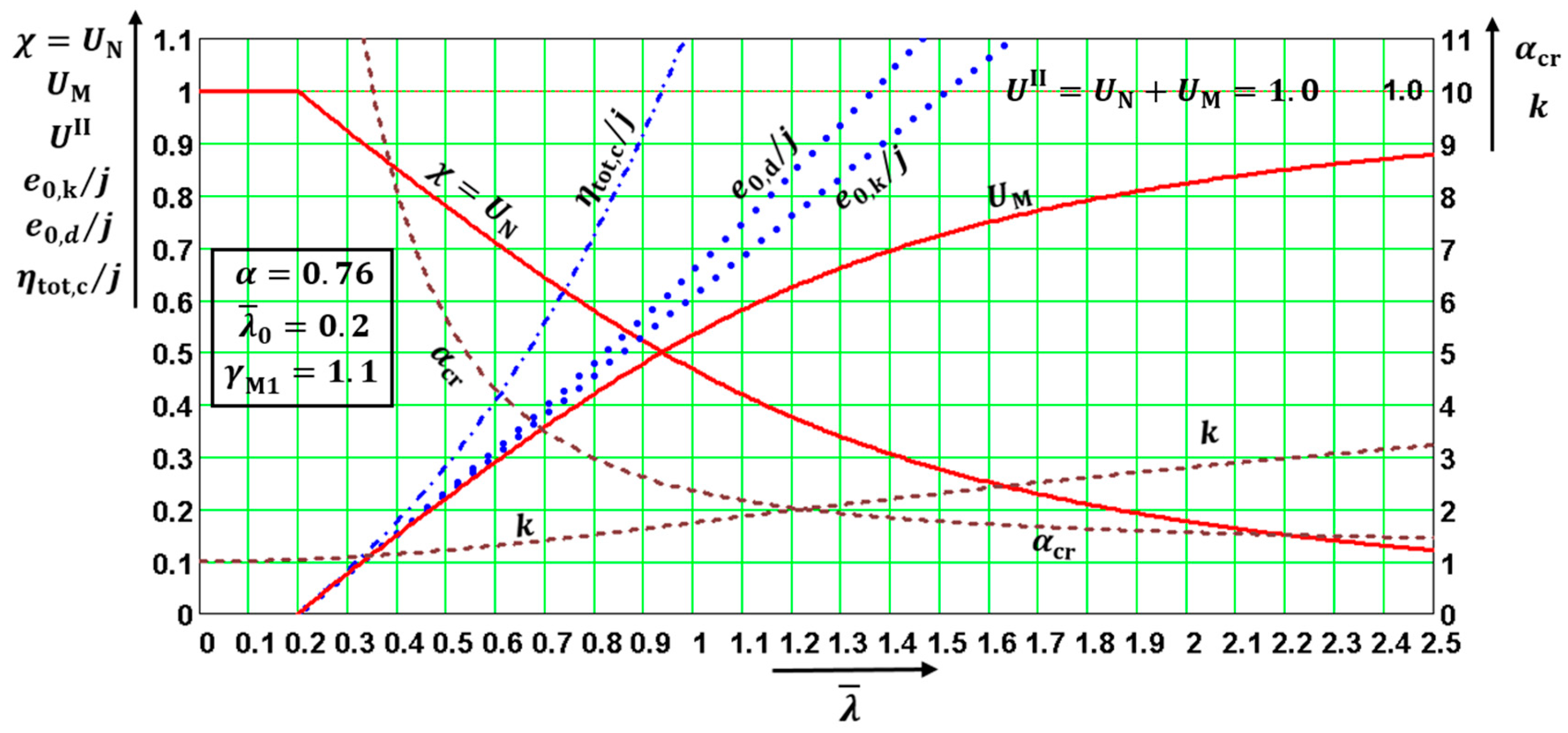
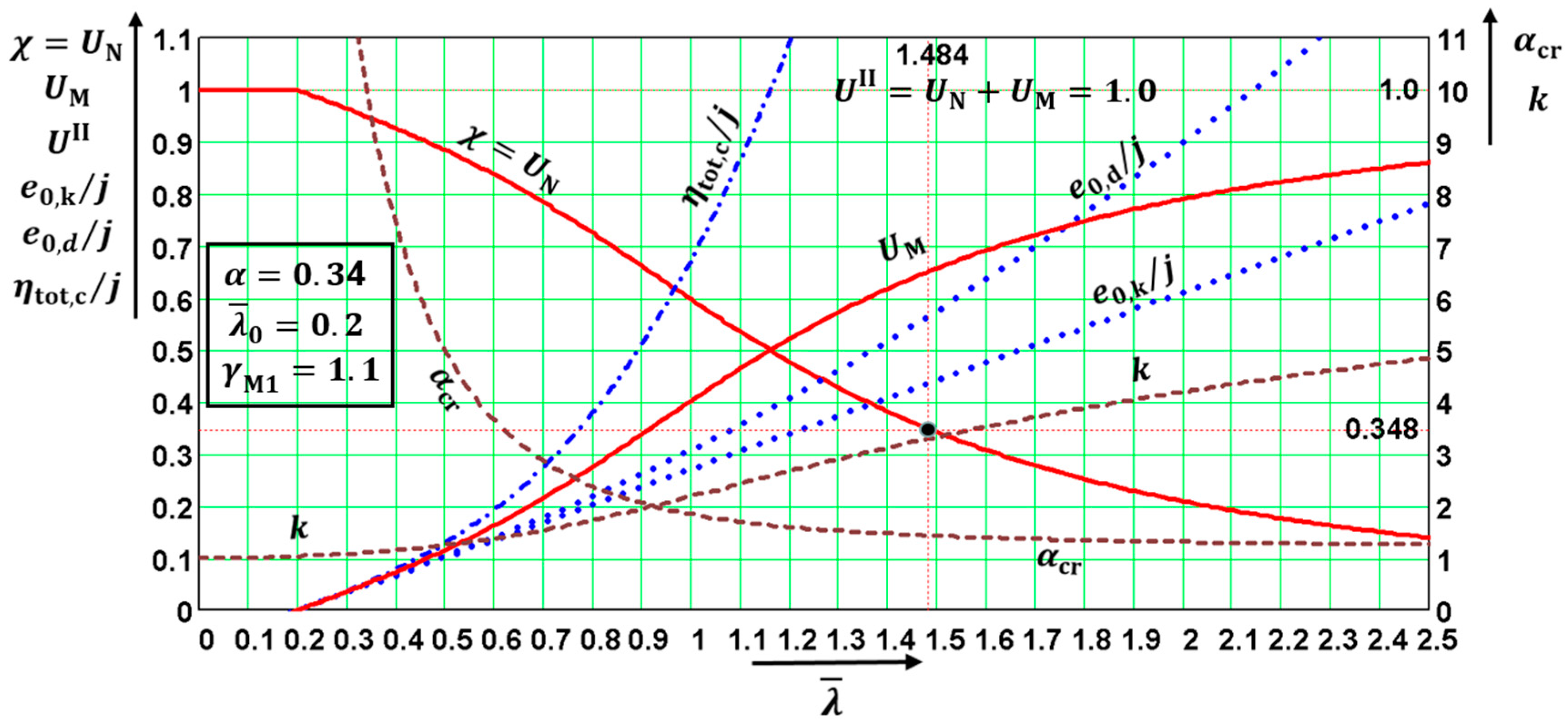
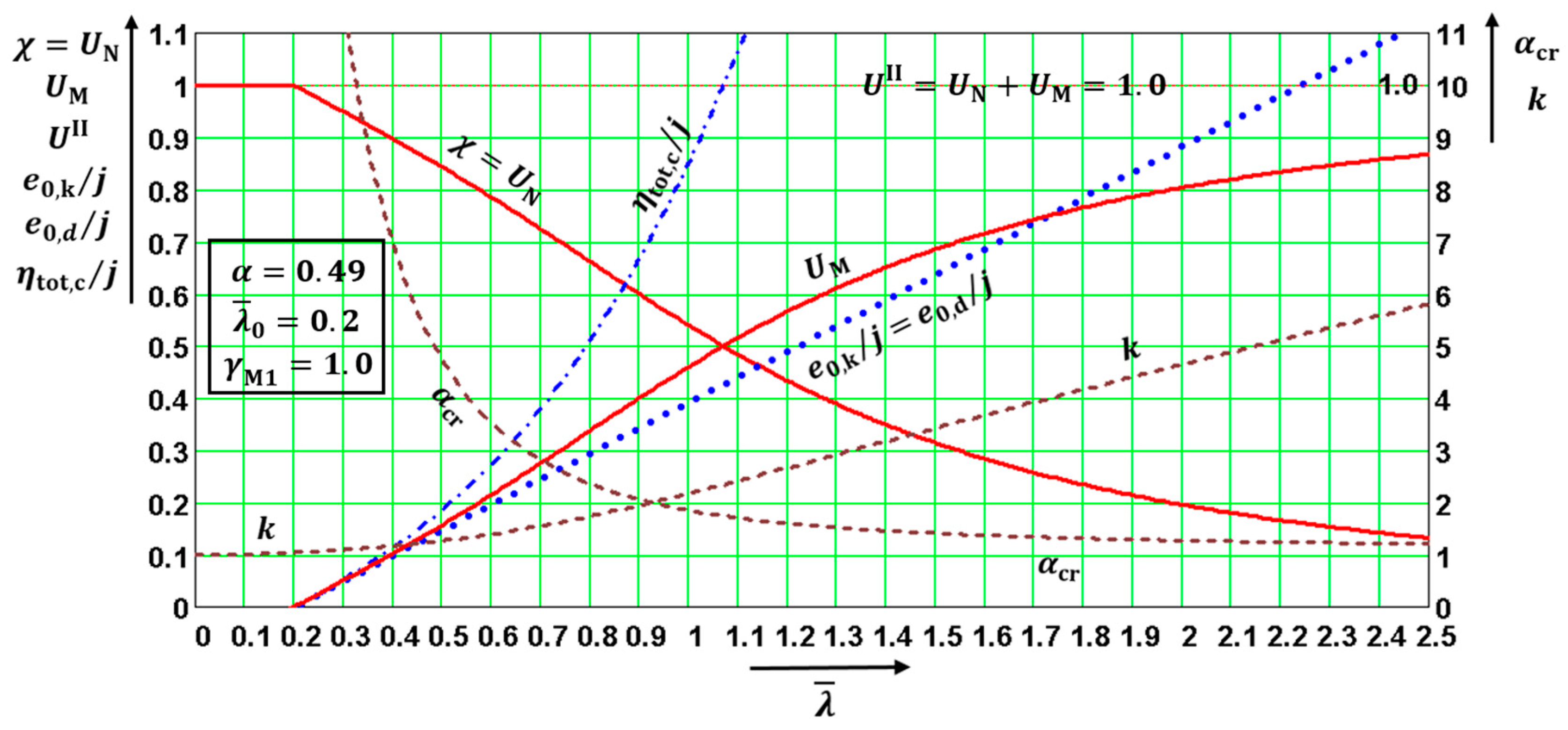
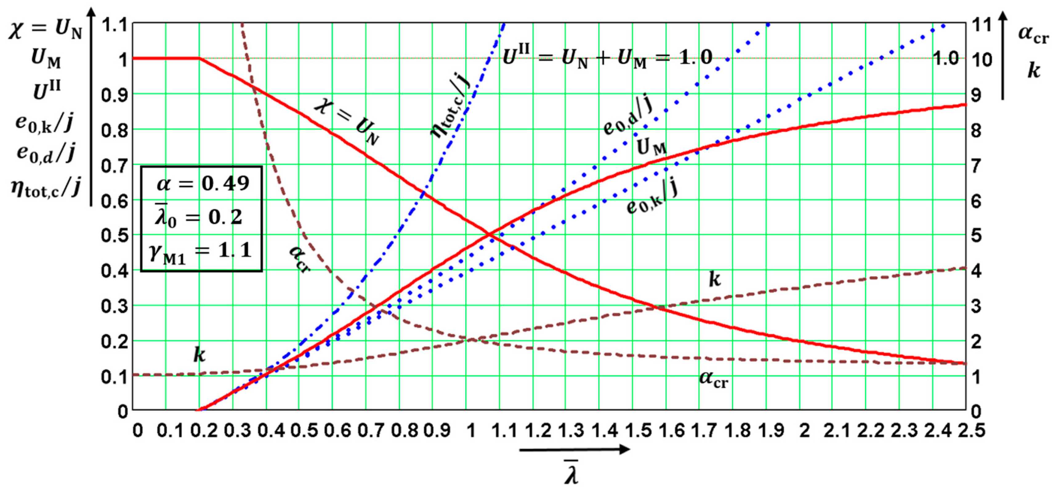
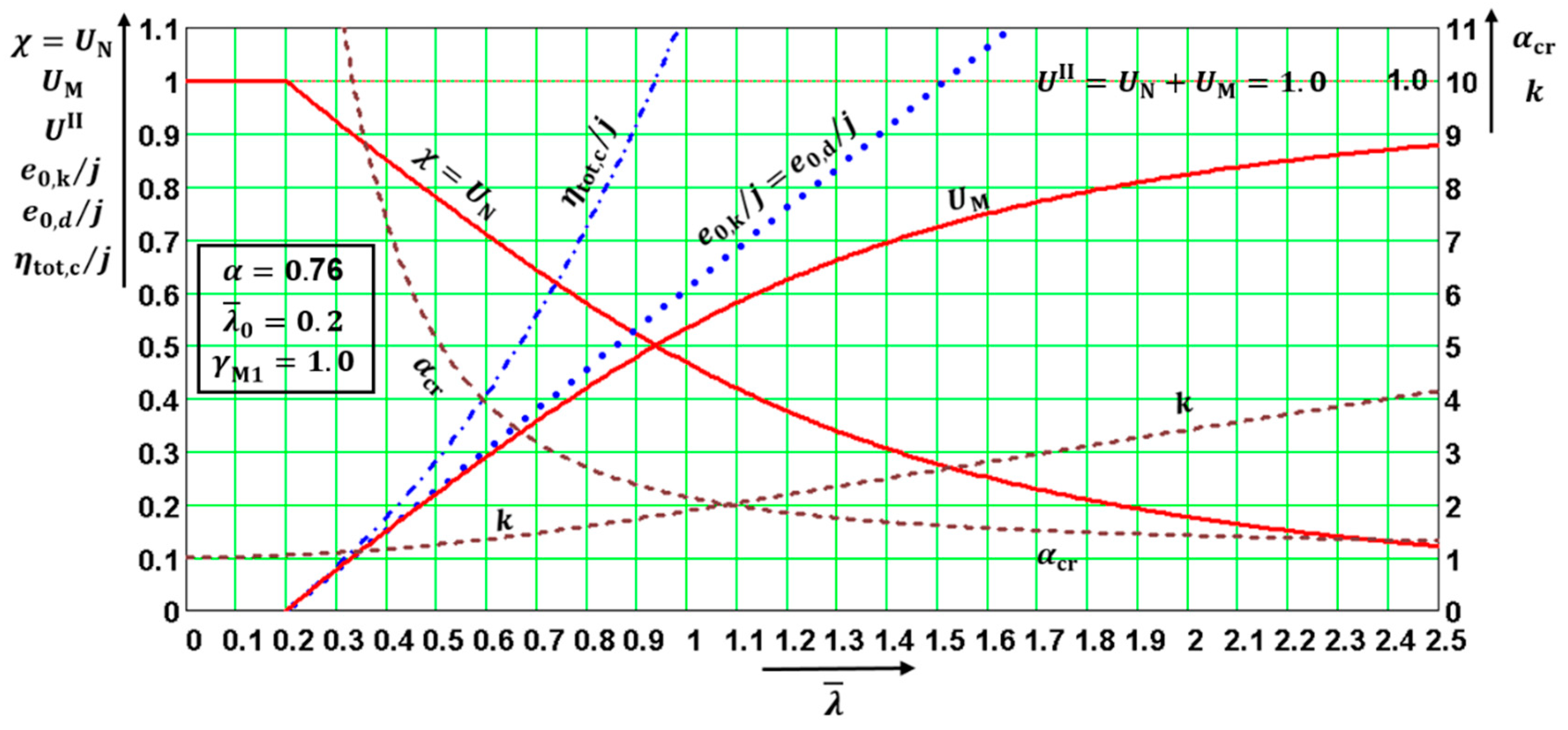
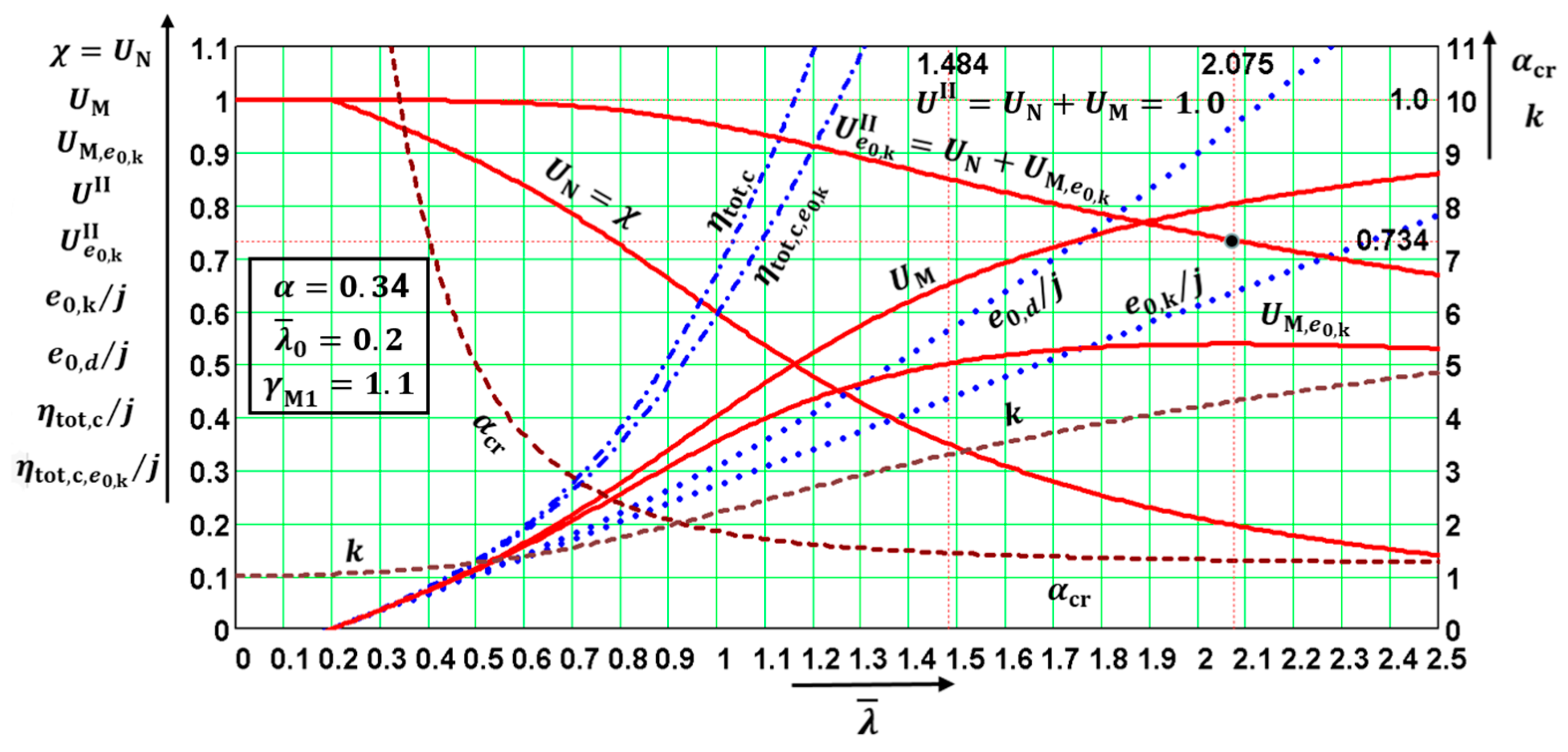
The quantities ${\eta }_{\mathrm{tot},\mathrm{c}}/j, U_{\mathrm{N}}, U_{\mathrm{M}} \mathrm{and} U$ are functions of only three parameters: $\alpha , \overline{\lambda ,} \mathrm{and} {\overline{\lambda }}_0$. The quantities ${\alpha }_{\mathrm{cr}}, k, U_{\mathrm{M},e_{0,\mathrm{k}}}, U_{e_{0,\mathrm{k}}}^{\mathrm{II}}, e_{0,\mathrm{d}}/j, {\eta }_{\mathrm{tot},\mathrm{c},e_{0,\mathrm{k}}}, \mathrm{and} {\eta }_{\mathrm{ad},\mathrm{d},\mathrm{c}}/j$ (not directly in all diagrams) depended on four parameters: $\alpha , \overline{\lambda }, {\overline{\lambda }}_0, \mathrm{and} {\gamma }_{\mathrm{M}1}$. This fact enabled the distributions of the above quantities to be drawn in the following diagrams, which were created for the values ${\overline{\lambda }}_0=0.2, {\gamma }_{\mathrm{M}1}=1.0; 1.1 \mathrm{and} \alpha =0.13; 0.21; 0.34; 0.49;\mathrm{and} 0.76.$ The values in diagrams were valid for $N_{\mathrm{Ed}}=N_{\mathrm{b},\mathrm{Rd}}=\chi A{f}_{\mathrm{y}}/ {\gamma }_{\mathrm{M}1}$ and, therefore, for both utility factors $U_{\mathrm{EMM}}=1.0$ and $U^{\mathrm{II}}=1.0$ if $e_{0,\mathrm{d}}$ was used in the calculation. Note that the diagrams have two vertical axes with different scales. The right one is valid for ${\alpha }_{\mathrm{cr}} \mathrm{and} k$.

The diagrams enable the determination of: (a) the amplitudes of all kinds of deformations, and (b) the influence of the second-order theory. The first-order analysis may be used for the structure if the increase in the relevant internal forces or moments, or any other change in structural behavior caused by deformations, can be neglected. This condition may be assumed fulfilled if the following criterion is met: ${\alpha }_{\mathrm{cr}}=N_{\mathrm{cr}}/N_{\mathrm{Ed}}\ge 10.$ This condition is fulfilled in the case of ${\gamma }_{\mathrm{M}1}=1.0$ $\left[ {\gamma }_{\mathrm{M}1}=1.1 \right]$ and for $\alpha =0.13$ when $\overline{\lambda }\le 0.319 \left[0.335\right];$ for $\alpha =0.21$ when $\overline{\lambda }\le 0.321 \left[0.337\right];$ for $\alpha =0.34$ when $\overline{\lambda }\le 0.323$ $\left[0.341\right];$ for $\alpha =0.49$ when $\overline{\lambda }\le 0.327 \left[0.345\right]$; and for $\alpha =0.76$ when $\overline{\lambda }\le 0.334 \left[0.353\right].$ The contribution of the bending moment $U_{\mathrm{M}}$ was greater than that of the normal force $U_{\mathrm{N}}$ for $\alpha =0.13$ when $\overline{\lambda }\ge 1.309;$ for $\alpha =0.21$ when $\overline{\lambda }\ge 1.248;$ for $\alpha =0.34$ when $\overline{\lambda }\ge 1.16;$ for $\alpha =0.49$ when $\overline{\lambda }\ge 1.07$; and for $\alpha =0.76$ when $\overline{\lambda }\ge 0.938.$ The design values of the relative amplitudes of additional deformations ${\eta }_{\mathrm{add}}\left(x\right)$ can be obtained from the diagrams as differences ${\eta }_{\mathrm{ad},\mathrm{d},\mathrm{c}}/j={\eta }_{\mathrm{tot},\mathrm{c}}/j-e_{0,\mathrm{d}}/j.$

The program FE-STAB [1] provided the following results for the input values from Numerical Example 1: (a) for the buckling perpendicular to the weak axis z–z, with the safety factor ${\gamma }_{\mathrm{M}1}=1.1,$ the value of axial force $N_{\mathrm{Ed}}=N_{\mathrm{b},\mathrm{Rd}}=859.584 \mathrm{kN}, \mathrm{and} e_{0,\mathrm{d}}=10.51 \mathrm{mm}:$ ${\alpha }_{\mathrm{cr}}=1.43439,$ ${\eta }_{\mathrm{ad},\mathrm{d},\mathrm{c}}=24.19 \mathrm{mm}, M_{\mathrm{c}}^{\mathrm{II}}=29.83 \mathrm{kNm}$. Compare these values to those in Table 4: (b) for $e_{0,\mathrm{k}}=8.09 \mathrm{mm}$, FE-STAB gives: ${\alpha }_{\mathrm{cr}}=1.43439,$ ${\eta }_{\mathrm{ad},\mathrm{d},\mathrm{c}}=18.62 \mathrm{mm}, \mathrm{and} M_{\mathrm{c}}^{\mathrm{II}}=22.96 \mathrm{kNm}.$ Compare these values to those in Equations (42) and (43). Consequently, $U_{e_{0,\mathrm{k}}}^{\mathrm{II}}=0.85$ (Equation (45)). The FE-STAB results confirm the correctness of the values in Table 4 and in Equations (41)–(45); (c) for safety factor ${\gamma }_{\mathrm{M}1}=1.0,$ a value of the axial force $N_{\mathrm{Ed}}=N_{\mathrm{b},\mathrm{Rd}}=945.543 \mathrm{kN}, \mathrm{and} e_{0,\mathrm{k}}=8.09 \mathrm{mm}$, FE-STAB gives: ${\alpha }_{\mathrm{cr}}=1.30402,$ ${\eta }_{\mathrm{ad},\mathrm{d},\mathrm{c}}=26.608 \mathrm{mm}, \mathrm{and} M_{\mathrm{c}}^{\mathrm{II}}=32.81 \mathrm{kNm}.$ Consequently,$U^{\mathrm{II}}=U_{\mathrm{N}}+U_{\mathrm{M}}=0.348+0.652=1.0.$ The same numerical results can be obtained with the above Equations (19)–(32) when safety factor ${\gamma }_{\mathrm{M}1}=1.0$ is used.

The formula $M_{\mathrm{Ed}}^{\mathrm{II}}=k{M}_{\mathrm{Ed}}^{\mathrm{I}}$ gives an exact value of $M_{\mathrm{Ed}}^{\mathrm{II}}$ under the condition that additive deformation is affine to the geometric initial imperfection in the form of the elastic buckling mode ${\eta }_{\mathrm{cr}}\left(x\right).$ The programs IQ 100 and FE-STAB enabled a simply supported column on both ends to be used as the initial imperfection, as well as the deformation in the form of a second-degree parabola, which did not differ much from the sinus half-wave form. Nevertheless, in this case, the formula $M_{\mathrm{Ed}}^{\mathrm{II}}=k{M}_{\mathrm{Ed}}^{\mathrm{I}}$ gave only an approximate value for $M_{\mathrm{Ed}}^{\mathrm{II}}$. Compare the obtained second-degree parabola “values $M_{\mathrm{z},\mathrm{Ed},\mathrm{c}}^{\mathrm{II}}=33.5857 \mathrm{kNm}$ and ${\eta }_{\mathrm{ad},\mathrm{c}}=27.427 \mathrm{mm}$ to the exact sinus half-wave” values 32.805 kNm and 26.601 mm, respectively. The exact values can be obtained from Equations (26) and (27) when the safety factor ${\gamma }_{\mathrm{M}1}=1.0$ is used. For some cases, using formula $M_{\mathrm{Ed}}^{\mathrm{II}}=k{M}_{\mathrm{Ed}}^{\mathrm{I}}$ is forbidden because it gives incorrect results. Employing the initial geometric imperfection in the form of the elastic buckling mode ${\eta }_{\mathrm{cr}}\left(x\right)$ substantially simplifies the calculations.

3. Unique Global and Local Initial (UGLI) Imperfection Method

3.1. Historical Development of the UGLI Imperfection Method

Chladný prepared Table B.1 for STN 73 140:1998 partly based on [2] to determine the imperfection equivalent of a member under compression, for which he calculated and proposed the values of relevant parameters based on his own study. The equivalent imperfection form corresponds to pre-standard ENV Eurocode 3 [2], which differs from the later EN Eurocode 3 drafts [3,4] and the current Eurocodes 3 and 9.

In October 2000, Chladný sent to Prof. J. Brozzetti comments on [2] and on [3] regarding the equivalent imperfection value of a member under compression. In the draft prEN Eurocode [3], the imperfection form corresponded to the pre-standard ENV Eurocode [2]. Consequently, the imperfection form was changed in the later prEN Eurocode 3 drafts. See [5] as well.

The list of references in [5] cites the work of Chladný E. (item [52] in [5]) as the only one from countries of the former Central and Eastern Europe and non-CEN members.

Until February 2004, the working draft prEN 1999-1-1 [6] did not contain provisions concerning the shape and value of a single equivalent for the global and local imperfections of a member under compression. For prEN 1999-1-1 [6], Baláž and Chladný also prepared a proposal for the clause containing the shape and amplitude of the equivalent geometrical UGLI imperfection of a member under compression. Chladný developed the proposal for EN 1999-1-1, which differs from that which was accepted in EN 1993-1-1 [7]. Baláž modified Chladný’s proposal by adding the absolute values and other changes used in the formulae in such a way that the formulae gave correct numerical results. In EN 1993-1-1 and in 5.3.2(11), instructions are given for determining the amplitude of the UGLI imperfection of compressed structures with a cross-section and a constant axial force along their length. In EN 1999-1-1 [8], the more general procedure is given in 5.3.2(11), which is also valid for members with a variable and/or non-uniform axial force. Baláž and Chladný sent their more general procedure to TC 250/SC9. Their proposal was accepted by prof. Torsten Höglund in Sweden, who was the head of Project Team PT Members in Subcommittee SC9, and by prof. Federico Mazzollani in Italy, who was the chairman of Subcommittee TC 250/SC9. The procedure can be found in the working drafts starting with draft prEN 1999-1-1, April 2004. The more general procedure by Baláž and Chladný was also accepted in the Slovak National Annex [9].

The above historical development has been described in detail by Baláž in the proceedings [10], where in Chapter 5, Chladný published his theory for the first time together with detailed numerical examples and applications in many areas. Chladný gave presentations in 2007 in courses for practicing designers and for people from universities. In the second edition of the proceedings [11], Baláž and Chladný corrected Chapter 5. In the courses for practicing designers and for people from universities, the 2010 presentations were given by Baláž because Chladný was ill.

Baláž derived Chladný’s method differently [12,13] and showed that the UGLI imperfection and its amplitude have a geometrical interpretation, which is helpful for practicing designers. The geometrical interpretation is valid only for structures with a cross-section and a constant axial force along their length.

Baláž asked Chladný to publish his theory in English. The UGLI imperfection method was published by Chladný and his daughter in English in [14,15], where more details about the method are found. Baláž’s contributions to the UGLI imperfection method are acknowledged by Chladný at the end of [15].

Baláž and Chladný improved some wording in EN 1993-1-1:2005 [7], Corrigenda AC2:2009, and EN 1999-1-1:2007 [8] in Amendment A1:2009.

The best formulation of the UGLI imperfection method prepared by Baláž and Chladný was used for several prEN 1999-1-1 drafts, and it may also be found in Clause 7.3.2(11) of the draft FprEN 1999-1-1:2022-01-14, document CEN/TC 250/SC 9 N 1047 [16]. The attempt by Baláž to unify the prEN 1993-1-1 drafts with the prEN 1999-1-1 drafts failed. German members of TC 250/SC 3 removed the safety factor ${\gamma }_{\mathrm{M}1}$ from the amplitude of the UGLI imperfection $e_{0\mathrm{d}}.$ The wording in Clause 7.3.6 of FprEN 1993-1-1:2021-11-26, document CEN/TC 250/SC 3 N 3504 [17], therefore differs from Clause 7.3.2(11) of draft FprEN 1999-1-1:2022-01-14. Compare Equation (7.7) in [16], containing safety factor ${\gamma }_{\mathrm{M}1}$, to Equation (7.19) in [17] without ${\gamma }_{\mathrm{M}1}$. The reasons presented during the Subcommittee TC 250/SC three meetings for the removal of ${\gamma }_{\mathrm{M}1}$ were as follows: (a) the amplitude $e_{0,\mathrm{k}}$ will be greater than $e_{0,\mathrm{d}}$ and the results will be on the safe side; (b) the influence of removing ${\gamma }_{\mathrm{M}1}$ is negligible; and (c) the change in the values of the equivalent bow imperfection $e_0$ in Clause 7.3.3.1 in [17], compared to the values of the equivalent bow imperfection $e_0$ in Clause 5.3.2.3b in [7], also influences the value of the amplitude of UGLI imperfection. These reasons cannot be accepted at all. The opposite is true, which is clearly explained in this paper.

A detailed explanation of the UGLI imperfection method and its geometrical interpretation can be found in [18].

An application of the UGLI imperfection method on the large Žďákov steel arch bridge is published in [19].

3.2. UGLI Imperfection Method Proposed by Baláž and Chladný for the Drafts of Eurocodes [16,17]

As an alternative to the second-order theory with the amplitude $e_0$ of the equivalent bow imperfection given in cl. 7.3.3.1(1) in [17], the shape of the elastic critical buckling mode, ${\eta }_{cr}\left(x\right)$, of the frame structure or the verified member can be applied as the unique global and local initial (UGLI) imperfection. The equivalent geometrical initial imperfection and its amplitude can be expressed in the following forms:

$${\eta }_{\mathrm{init},\mathrm{m}}\left(x\right)=e_{0\mathrm{d},\mathrm{m}}\frac{N_{\mathrm{cr},\mathrm{m}}}{E{I}_{\mathrm{m}}\left|{\eta }_{cr}^{″}\left(x_{\mathrm{m}}\right)\right|}{\eta }_{\mathrm{cr}}\left(x\right), {\eta }_{0,\mathrm{m}}=e_{0\mathrm{d},\mathrm{m}}\frac{N_{\mathrm{cr},\mathrm{m}}}{E{I}_{\mathrm{m}}\left|{\eta }_{cr}^{″}\left(x_{\mathrm{m}}\right)\right|},$$

(46)

where the design value of $e_{0\mathrm{d},\mathrm{m}}$ is given by:

$$e_{0\mathrm{d},\mathrm{m}}={\alpha }_{\mathrm{m}}\left({\overline{\lambda }}_{\mathrm{m}}-{\overline{\lambda }}_0\right)\frac{M_{\mathrm{c},\mathrm{Rk},\mathrm{m}}}{N_{\mathrm{c},\mathrm{Rk},\mathrm{m}}}\frac{1-\frac{{\chi }_{\mathrm{m}}{\overline{\lambda }}_m^2}{{\gamma }_{\mathrm{M}1}}}{1-{\chi }_{\mathrm{m}}{\overline{\lambda }}_m^2}, \mathrm{for} {\overline{\lambda }}_{\mathrm{m}}>{\overline{\lambda }}_0.$$

(47)

where $x_{\mathrm{m}}$ denotes the critical cross-section of either the frame structure or the verified member (see Note 5); $m$ is the index that indicates belonging to the critical cross-section; ${\alpha }_{\mathrm{m}}$ is the imperfection factor for the relevant buckling curve; ${\overline{\lambda }}_{\mathrm{m}}=\sqrt{\frac{N_{\mathrm{c},\mathrm{Rk},\mathrm{m}}}{N_{\mathrm{cr},\mathrm{m}}} }$ is the relative slenderness of either the frame structure or the verified member and of the equivalent member (see Note 2); ${\overline{\lambda }}_0$ is the limit of the horizontal plateau for the relevant buckling curve; ${\chi }_{\mathrm{m}}$ is the reduction factor for the relevant buckling curve and slenderness ${\overline{\lambda }}_{\mathrm{m}}; N_{\mathrm{cr},\mathrm{m}}={\alpha }_{\mathrm{cr},\mathrm{m}}{N}_{\mathrm{Ed},\mathrm{m}}$ is the value of the axial force in the critical cross-section, $x_{\mathrm{m}}$, when the elastic critical buckling is reached, and it is also the critical axial force for the equivalent member; ${\alpha }_{\mathrm{cr} }$ is the minimum force amplifier for the axial force configuration $N_{\mathrm{Ed}}$ in members to reach the structure’s elastic critical buckling; $M_{\mathrm{c},\mathrm{Rk},\mathrm{m}}$ is the characteristic moment resistance of the cross-section, $x_{\mathrm{m}}; N_{\mathrm{c},\mathrm{Rk},\mathrm{m}}$ is the characteristic normal force resistance of the cross-section, $x_{\mathrm{m}}; \mathrm{and} E{I}_{\mathrm{m}}\left|{\eta }_{cr}^{″}\left(x_{\mathrm{m}}\right)\right|$ is the value in the critical cross-section, $x_{\mathrm{m}}$, of the bending moments, which would be necessary to bend the structure (in the state without axial forces) in the form of the buckling mode.

Note 1: Formula (46) is based on the requirement that an imperfection,${\eta }_{\mathrm{init},\mathrm{m}}\left(x\right),$ in the shape of the elastic buckling mode, ${\eta }_{\mathrm{cr}}\left(x\right)$, should have the same maximum curvature as assumed for the equivalent member method in $\left(N_{\mathrm{Ed}}\le N_{\mathrm{b},\mathrm{Rd}}\right)$. Therefore, the buckling resistance of the uniform members loaded in axial compression, and calculated with the imperfection according to (46) and for second-order effects, is identical with the value of $N_{\mathrm{b},\mathrm{Rd}}=\chi A{f}_{\mathrm{y}}/ {\gamma }_{\mathrm{M}1}.$ The imperfection, ${\eta }_{\mathrm{init},\mathrm{m}}\left(x\right)$, in the shape of the elastic critical buckling mode is generally applicable to all members under compression and to frames buckling in their plane. It is especially suitable for members with cross-sectional characteristics and/or an axial force that is not constant along their length, and also for frames containing such members.

Note 2: The equivalent member has pinned ends, and its cross-section and axial force are the same as in the critical cross-section, $x_{\mathrm{m}}$, of the frame. Its length is such that the critical force equals the axial force in the critical cross-section, $x_{\mathrm{m}}$, upon the critical loading of the structure.

Note 3: To calculate the amplifier, ${\alpha }_{\mathrm{cr}}$, the members of the structure may be considered to be loaded by axial forces, $N_{\mathrm{Ed}}$, from the first-order elastic analysis of the structure.

Note 4: The formula $E{I}_{\mathrm{m}}\left|{\eta }_{cr}^{″}\left(x_{\mathrm{m}}\right)\right|$ in (46) may be replaced with $|M_{{\mathsf{\eta }}_{\mathrm{cr}},\mathrm{m}}^{\mathrm{II}}|\left({\alpha }_{\mathrm{cr},\mathrm{m} }-1\right),$ where $M_{{\mathsf{\eta }}_{\mathrm{cr}},\mathrm{m}}^{\mathrm{II}}$ is the bending moment in the cross-section, $x_{\mathrm{m}}$, calculated by the second-order analysis of the structure with the imperfection in the shape of the elastic critical buckling mode ${\eta }_{\mathrm{cr}}\left(x\right)$ and with an arbitrary value for the maximum amplitude ${\left|{\eta }_{\mathrm{cr}}\left(x\right)\right|}_{\max }$.

Note 5: The position of the critical cross-section, $x_{\mathrm{m}},$ should be generally determined by an iterative procedure. The selected position for the critical cross-section, $x_{\mathrm{m}}$, is correct if the utilization in the selected position, $x_{\mathrm{m}}$, is greater than the utilization at all the other points, $x$, of the structure.

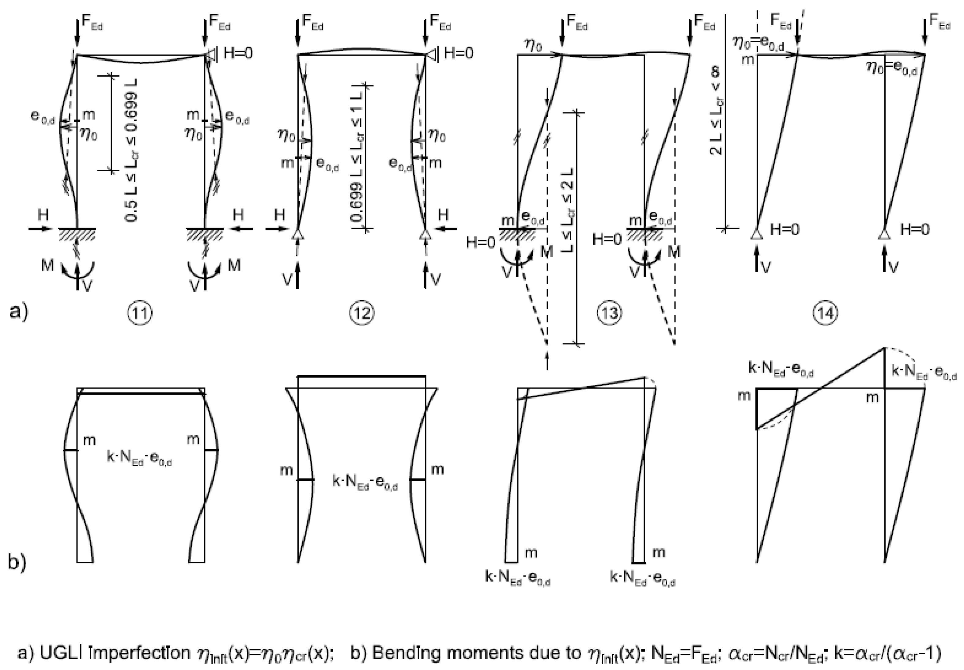
Effect of ${\eta }_{\mathrm{init},\mathrm{m}}\left(x\right)$ imperfection.

Deflexion ${\eta }^{\mathrm{II}}\left(x\right)$, as the effect of the imperfection ${\eta }_{\mathrm{cr}}\left(x\right)$ on the compressed member, is calculated using the second-order analysis as follows [14]:

$${\eta }^{\mathrm{II}}\left(x\right)=\frac{{\eta }_{\mathrm{cr}}\left(x\right)}{{\alpha }_{\mathrm{cr}}\left(x\right)-1},$$

(48)

where generally, for a non-uniform member with non-uniform distribution of axial force:

$${\alpha }_{\mathrm{cr}}\left(x\right)=\frac{N_{\mathrm{cr}}\left(x\right)}{N_{\mathrm{Ed}}\left(x\right)}.$$

(49)

The maximum of the equivalent geometrical initial imperfection ${\eta }_{\mathrm{init},\mathrm{m}}\left(x\right)$ is given by:

$${\left|{\eta }_{\mathrm{init},\mathrm{m}}\left(x\right)\right|}_{\max }=e_{0\mathrm{d},\mathrm{m}}\frac{N_{\mathrm{cr},\mathrm{m}}}{E{I}_{\mathrm{m}}\left|{\eta }_{cr}^{″}\left(x_{\mathrm{m}}\right)\right|}{\left|{\eta }_{\mathrm{cr}}\left(x\right)\right|}_{\max }=\frac{{\alpha }_{\mathrm{m}}\left({\overline{\lambda }}_{\mathrm{m}}-{\overline{\lambda }}_0\right)}{{\overline{\lambda }}_{\mathrm{m}}^2}\frac{1-\frac{{\chi }_{\mathrm{m}}{\overline{\lambda }}_m^2}{{\gamma }_{\mathrm{M}1}}}{1-{\chi }_{\mathrm{m}}{\overline{\lambda }}_m^2}\frac{M_{\mathrm{c},\mathrm{Rk},\mathrm{m}}{\left|{\eta }^{\mathrm{II}}\left(x\right)\right|}_{\max }}{|M_{{\mathsf{\eta }}_{\mathrm{cr}},\mathrm{m}}^{\mathrm{II}}|}.$$

(50)

$M_{{\mathsf{\eta }}_{\mathrm{cr}}}^{\mathrm{II}}\left(\mathrm{x}\right)$ is the bending moment in the structure, with the geometry influenced by the initial imperfection in the form of the elastic buckling mode ${\eta }_{\mathrm{cr}}\left(x\right)$ with an arbitrary value of amplitude ${\left|{\eta }_{\mathrm{cr}}\left(x\right)\right|}_{\max }$.

The bending moment at the critical cross-section $m$ of the verified member or the structure initially bent into the shape of the initial imperfection ${\eta }_{\mathrm{init},\mathrm{m}}\left(x\right)$ is as follows:

$$\begin{array}{c}{M}_{{\mathsf{\eta }}_{\mathrm{init},\mathrm{m}}}^{\mathrm{II}}\left(x\right)=\frac{{\left|{\eta }_{\mathrm{init},\mathrm{m}}\left(x\right)\right|}_{\max }}{{\left|{\eta }_{\mathrm{cr}}\left(x\right)\right|}_{\max }}{M}_{{\mathsf{\eta }}_{\mathrm{cr}}}^{\mathrm{II}}\left(\mathrm{x}\right)=\frac{{\left|{\eta }_{\mathrm{init},\mathrm{m}}\left(x\right)\right|}_{\max }}{{\left|{\eta }_{\mathrm{ad}}\left(x\right)\right|}_{\max }\left[{\alpha }_{\mathrm{cr}}\left(x\right)-1\right]}{M}_{{\mathsf{\eta }}_{\mathrm{cr}}}^{\mathrm{II}}\left(\mathrm{x}\right)\\ =\frac{{\alpha }_{\mathrm{m}}\left({\overline{\lambda }}_{\mathrm{m}}-{\overline{\lambda }}_0\right)}{{\overline{\lambda }}_{\mathrm{m}}^2\left[{\alpha }_{\mathrm{cr}}\left(x\right)-1\right]}\frac{1-\frac{{\chi }_{\mathrm{m}}{\overline{\lambda }}_{\mathrm{m}}^2}{{\gamma }_{\mathrm{M}1}}}{1-{\chi }_{\mathrm{m}}{\overline{\lambda }}_{\mathrm{m}}^2}\frac{M_{\mathrm{c},\mathrm{Rk},\mathrm{m}}}{\left|M_{{\mathsf{\eta }}_{\mathrm{cr}},\mathrm{m}}^{\mathrm{II}}\right|}{M}_{{\mathsf{\eta }}_{\mathrm{cr}}}^{\mathrm{II}}\left(\mathrm{x}\right).\end{array}$$

(51)

The utilization is given by:

$$U_{{\mathsf{\eta }}_{\mathrm{init},\mathrm{m}}}\left(x\right)=U_{{\mathrm{N}}_{\mathrm{Ed}}}\left(x\right)+U_{{\mathrm{M}}_{{\mathsf{\eta }}_{\mathrm{init},\mathrm{m}}}}\left(x\right)=\frac{N_{\mathrm{Ed}}\left(x\right)}{N_{\mathrm{c},\mathrm{Rd}}\left(x\right)}+\frac{M_{{\mathsf{\eta }}_{\mathrm{init},\mathrm{m}}}^{\mathrm{II}}\left(x\right)}{M_{\mathrm{c},\mathrm{Rd}}\left(x\right)},$$

(52)

$$U_{{\mathrm{M}}_{{\mathsf{\eta }}_{\mathrm{init},\mathrm{m}}}}\left(x\right)=\frac{{\alpha }_{\mathrm{m}}\left({\overline{\lambda }}_{\mathrm{m}}-{\overline{\lambda }}_0\right)}{{\overline{\lambda }}_{\mathrm{m}}^2\left[{\alpha }_{\mathrm{cr}}\left(x\right)-1\right]}\frac{1-\frac{{\chi }_{\mathrm{m}}{\overline{\lambda }}_{\mathrm{m}}^2}{{\gamma }_{\mathrm{M}1}}}{1-{\chi }_{\mathrm{m}}{\overline{\lambda }}_{\mathrm{m}}^2}\frac{M_{\mathrm{c},\mathrm{Rk},\mathrm{m}}}{\left|M_{{\mathsf{\eta }}_{\mathrm{cr}},\mathrm{m}}^{\mathrm{II}}\right|}\frac{M_{{\mathsf{\eta }}_{\mathrm{cr}}}^{\mathrm{II}}\left(\mathrm{x}\right)}{M_{\mathrm{c},\mathrm{Rd}}\left(x\right)}.$$

(53)

In Equation (53), the plastic resistance of the cross-section $M_{\mathrm{pl},\mathrm{c},\mathrm{Rd}}\left(x\right)=W_{\mathrm{pl}}\left(x\right)f_{\mathrm{y}}/{\gamma }_{\mathrm{M}1}$ may be used for Class 1 and 2 cross-sections instead of $M_{\mathrm{el},\mathrm{c},\mathrm{Rd}}\left(x\right)=W_{\mathrm{el}}\left(x\right)f_{\mathrm{y}}/{\gamma }_{\mathrm{M}1}$.

The utilization at the critical cross-section $x_{\mathrm{m}}$ is given by:

$$U_{{\mathrm{M}}_{{\mathsf{\eta }}_{\mathrm{init},\mathrm{m}}}}\left(x_{\mathrm{m}}\right)=\frac{{\alpha }_{\mathrm{m}}\left({\overline{\lambda }}_{\mathrm{m}}-{\overline{\lambda }}_0\right)}{{\overline{\lambda }}_{\mathrm{m}}^2\left[{\alpha }_{\mathrm{cr}}\left(x\right)-1\right]}\frac{1-\frac{{\chi }_{\mathrm{m}}{\overline{\lambda }}_{\mathrm{m}}^2}{{\gamma }_{\mathrm{M}1}}}{1-{\chi }_{\mathrm{m}}{\overline{\lambda }}_{\mathrm{m}}^2}{\gamma }_{\mathrm{M}1}.$$

(54)

For the elastic cross-sectional resistance of the uniform member with a uniform distribution of axial force when $N_{\mathrm{Ed}}=N_{\mathrm{b},\mathrm{Rd}}=\frac{\chi A{f}_{\mathrm{y}}}{{\gamma }_{\mathrm{M}1}},$ Equation (54) may be simplified in the form of Equation (31):

$$U_{{\mathrm{M}}_{{\mathsf{\eta }}_{\mathrm{init},\mathrm{m}}}}\left(x_{\mathrm{m}}\right)=\frac{\alpha \left(\overline{\lambda }-{\overline{\lambda }}_0\right)}{1-\chi {\overline{\lambda }}^2} \chi .$$

(55)

3.3. Numerical Examples 2a and 2b

(a) Numerical Example 2a.

The buckling perpendicular to axis z–z of the column simply supported at both ends was investigated, which was solved in Numerical Example 1 by two other methods. The input values were taken from Numerical Example 1. The axial force $N_{\mathrm{Ed}}=N_{\mathrm{b},\mathrm{Rd}}=859.584 \mathrm{kN}$ acted on the column with length $L=12 \mathrm{m}$ and simply supported at both member ends, with a uniform cross-section IPE 500 made from S235 steel. For this case, the calculation according to the UGLI imperfection method gave identical results as the calculation according to the second-order theory in Table 4. That is why all the steps of the calculation according to the UGLI imperfection method described above were applied for the more general case, in which the same column was fixed at the bottom and its upper end was simply supported. See the next numerical example, 2b.

(b) Numerical Example 2b for the column fixed at the bottom with its simply supported upper end.

The characteristic equation for the given boundary equation is:

$$\tan \epsilon =\epsilon .$$

(56)

The solution of the characteristic equation is $\epsilon =4.493409$.

The buckling length factor ${\beta }_{\mathrm{z}}=\frac{\pi }{\epsilon }=0.699.$ The buckling length $L_{\mathrm{cr},\mathrm{z}}={\beta }_{\mathrm{z}}L=0.699·12=8.39 \mathrm{m}$.

The critical force $N_{cr,z}={\pi }^{2}E{I}_{\mathrm{z}}/L_{\mathrm{cr},\mathrm{z}}^2=630.708 \mathrm{kN}; E=210,000 \mathrm{MPa}$.

The characteristic resistance of cross-section IPE 500 was $f_{\mathrm{y}}=235 \mathrm{MPa}$.

$$N_{\mathrm{c},\mathrm{Rk}}=A{f}_{\mathrm{y}}=2714.72 \mathrm{kN}.$$

(57)

The relative slenderness is given by:

$${\overline{\lambda }}_{\mathrm{m}}=\sqrt{\frac{N_{\mathrm{c},\mathrm{Rk},\mathrm{m}}}{N_{\mathrm{cr},\mathrm{m}}}}=2.075.$$

(58)

For the buckling curve “a”, the imperfection factor ${\alpha }_{\mathrm{m}}=0.34$.

The reduction factor ${\chi }_{\mathrm{m}}$ is given by:

$${\varphi }_{\mathrm{m}}=0.5\left[1+{\alpha }_{\mathrm{m}}\left({\overline{\lambda }}_{\mathrm{m}}-{\overline{\lambda }}_0\right)+{\overline{\lambda }}_{\mathrm{m}}^2\right]=2.971, {\chi }_{\mathrm{m}}=\frac{1}{{\varphi }_{\mathrm{m}}+\sqrt{{\varphi }_{\mathrm{m}}^2-{\overline{\lambda }}_{\mathrm{m}}^2}}0.196.$$

(59)

For the force $N_{\mathrm{Ed}}=N_{\mathrm{b},\mathrm{Rd}},$ the EM method gives the utility factor:

$$N_{\mathrm{Ed}}=N_{\mathrm{b},\mathrm{Rd}}=\frac{{\chi }_{\mathrm{m}}A{f}_{\mathrm{y}}}{1.1}=\frac{0.196 · 115.52{ \mathrm{cm}}^2 · 235 \mathrm{MPa}}{1.1}=484.173 \mathrm{kN}, U_{\mathrm{EMM}}=\frac{N_{\mathrm{Ed}}}{N_{\mathrm{b},\mathrm{Rd}}}=1.0.$$

(60)

The UGLI imperfection method gives:

$${\alpha }_{\mathrm{cr}}=\frac{N_{\mathrm{cr}}}{N_{\mathrm{Ed}}}=1.3026,$$

(61)

$$k=\frac{1}{1-\frac{1}{{\alpha }_{\mathrm{cr}}}}=4.304,$$

(62)

$$e_{0,\mathrm{k},\mathrm{m}}={\alpha }_{\mathrm{m}}\left({\overline{\lambda }}_{\mathrm{m}}-{\overline{\lambda }}_0\right) \frac{M_{\mathrm{c},\mathrm{Rk}}}{N_{\mathrm{c},\mathrm{Rk}}}={\alpha }_{\mathrm{m}}\left({\overline{\lambda }}_{\mathrm{m}}-{\overline{\lambda }}_0\right) \frac{W_z}{A}=11.819 \mathrm{mm},$$

(63)

$$e_{0,\mathrm{d},\mathrm{m}}=e_{0,\mathrm{k},\mathrm{m}}\frac{1-\frac{{\chi }_{\mathrm{m}}{\overline{\lambda }}_{\mathrm{m}}^2}{{\gamma }_{\mathrm{M}1}}}{1-{\chi }_{\mathrm{m}}{\overline{\lambda }}_{\mathrm{m}}^2}=17.651 \mathrm{mm}.$$

(64)

The eigenfunction of the buckling mode and its first derivation are given by:

$${\overline{\eta }}_{\mathrm{cr}}\left(x\right)=\left[\left(1-\cos \frac{\epsilon x}{L}\right)\epsilon +\sin \frac{\epsilon x}{L}-\frac{\epsilon x}{L}\right],$$

(65)

$${\overline{\eta }}_{\mathrm{cr}}^{\prime }\left(x\right)=\frac{{\epsilon }^2}{L}\sin \frac{\epsilon x}{L}+\frac{\epsilon }{L}\left(\cos \frac{\epsilon x}{L}-1 \right).$$

(66)

The maximum of function ${\overline{\eta }}_{\mathrm{cr}}\left(x\right)$ in section $x_{\mathrm{m}}=7.22 \mathrm{m}$, which was found from the condition ${\overline{\eta }}_{\mathrm{cr}}^{\prime }\left(x\right)=0$. The amplitude of ${\overline{\eta }}_{\mathrm{cr}}\left(x\right)$ is $C={\overline{\eta }}_{\mathrm{cr},\max }={\overline{\eta }}_{\mathrm{cr}}\left(x_{\mathrm{m}}\right)=6.2832.$ It was not necessary. Nevertheless, below the normalized eigenfunction, it was used with an amplitude equaling 1.0:

$${\eta }_{cr}\left(x\right)=\frac{1}{C}\left[\left(1-\cos \frac{\epsilon x}{L}\right)\epsilon +\sin \frac{\epsilon x}{L}-\frac{\epsilon x}{L}\right],$$

(67)

$${\eta }_{cr}^{″}\left(x\right)=\frac{1}{C}\left(\frac{{\epsilon }^3}{L^2}\cos \frac{\epsilon x}{L}-\frac{{\epsilon }^2}{L^2}\sin \frac{\epsilon x}{L}\right),$$

(68)

$${\eta }_{cr}^{‴}\left(x\right)=\frac{1}{C}\left(-\frac{{\epsilon }^4}{L^3}\sin \frac{\epsilon x}{L}-\frac{{\epsilon }^3}{L^3}\cos \frac{\epsilon x}{L}\right).$$

(69)

The maximum of function ${\eta }_{cr}^{″}\left(x\right)$ in section $x_{\mathrm{m}}=7.805 \mathrm{m}$, which was found from condition ${\eta }_{cr}^{‴}\left(x\right)=0$.

The amplitude of the equivalent geometrical initial imperfection was obtained after inserting the relevant values in Equation (50):

$$\begin{array}{c}{\left|{\eta }_{\mathrm{init},\mathrm{m}}\left(x\right)\right|}_{\max }={\eta }_0=e_{0\mathrm{d},\mathrm{m}}\frac{N_{\mathrm{cr},\mathrm{m}}}{E{I}_{\mathrm{m}}\left|{\eta }_{cr}^{″}\left(x_{\mathrm{m}}\right)\right|}{\left|{\eta }_{\mathrm{cr}}\left(x\right)\right|}_{\max }\\ =17.651 \mathrm{mm}\frac{630.708 \mathrm{kN}}{E · 2142 {\mathrm{cm}}^4 · \left|{\eta }_{cr}^{″}\left(7.805 \mathrm{m}\right)\right|}1.0=24.092 \mathrm{mm}.\end{array}$$

(70)

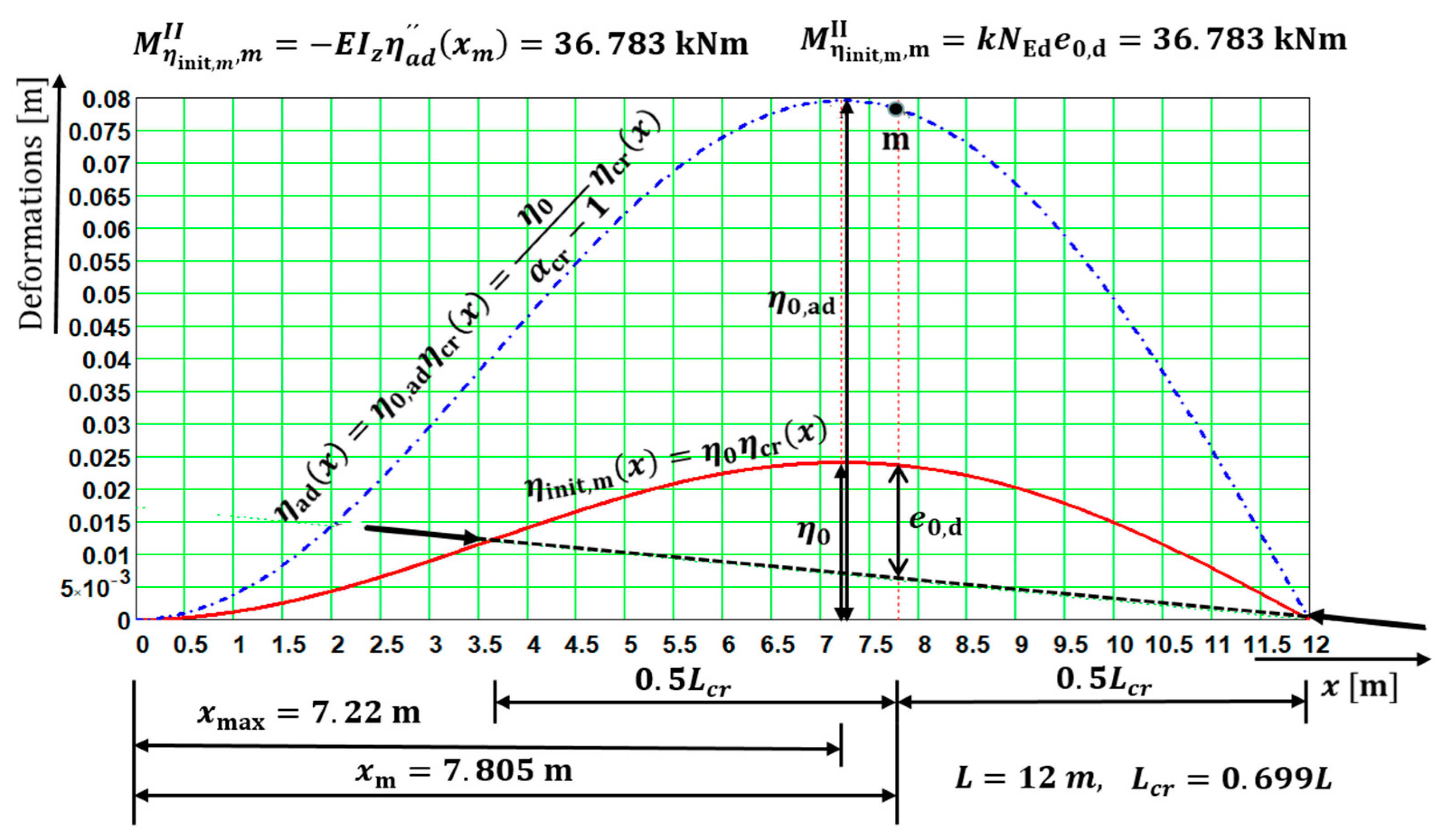
The amplitude of the additional deformation ${\eta }_{\mathrm{ad}}\left(x\right)$ is given by the following (see Figure 14):

$${\eta }_{0,\mathrm{ad}}=\frac{{\eta }_0}{{\alpha }_{\mathrm{cr}}-1}=79.6 \mathrm{mm}.$$

(71)

For the equivalent member with an initial imperfection, the bending moment $M_{{\mathsf{\eta }}_{\mathrm{init},\mathrm{m}},\mathrm{m}}^{\mathrm{II}}$ in the ultimate limit state is $M_{{\mathsf{\eta }}_{\mathrm{init},\mathrm{m}},\mathrm{m}}^{\mathrm{II}}=M_{{\mathsf{\eta }}_{\mathrm{init},\mathrm{m}},\max }^{\mathrm{II}}=k{N}_{\mathrm{Ed}}{e}_{0,\mathrm{d}}.$

$$\begin{array}{c}{M}_{{\mathsf{\eta }}_{\mathrm{init},\mathrm{m}},\mathrm{m}}^{\mathrm{II}}=k{N}_{\mathrm{Ed},\mathrm{m}}{e}_{0\mathrm{d},\mathrm{m}}=4.304 · 484.173 \mathrm{kN} · 17.651 \mathrm{mm}\\ =\mathrm{k}{M}_{{\mathsf{\eta }}_{\mathrm{init},\mathrm{m}},\mathrm{m}}^{\mathrm{I}}=4.304 · 8.546 \mathrm{kNm}=36.783 \mathrm{kNm}.\end{array}$$

(72)

The above results were confirmed by the computer program IQ 100 [20], see

Table 5. Program IQ 100 results. Compare them to the values in Equations (71) and (72), and to Figure 14.

${\mathit{M}}_{{\mathsf{\eta }}_{\mathbf{c}\mathbf{r}}}^{\mathbf{II}}\left(\mathit{x}\right)$(kNm)	${\mathit{\eta }}_{\mathbf{c}\mathbf{r}}\left(\mathit{x}\right) \left(\mathbf{mm}\right)$	$\mathit{x}$ (mm)	${\mathit{\eta }}_{\mathbf{a}\mathbf{d}}\left(\mathit{x}\right) \left(\mathbf{mm}\right)$	${\mathit{M}}_{{\mathsf{\eta }}_{\mathbf{init},\mathbf{m}}}^{\mathbf{II}}\left(\mathit{x}\right)$(kNm)
0.45098	0.0	0	0.0	35.9094
0.36261	0.0686	1.2	5.46207	28.8735
0.20226	0.25134	2.4	20.0129	16.1052
0.00175	0.49774	3.6	39.6332	0.13957
−0.1991	0.7447	4.8	59.2975	−15.8538
−0.36043	0.92899	6.0	73.9714	−28.6996
−0.4502	0.99982	7.2	79.6112	−35.8477
−0.45097	0.99984$\approx$1.0	${\mathit{x}}_{\max } =$7.22	${\mathbf{\eta }}_{\mathbf{0}.\mathbf{a}\mathbf{d}}=$79.6129	−35.9086
−0.46201	0.98249	${\mathit{x}}_{\mathbf{m}}=$7.805	78.2314	${\mathit{M}}_{{\mathsf{\eta }}_{\mathrm{init}.\mathbf{m}}.\mathbf{m}}^{\mathbf{II}}=$36.788
−0.45059	0.92893	8.4	73.967	−35.8788
−0.36153	0.71621	9.6	57.029	−28.7868
−0.20068	0.38969	10.8	31.0295	−15.9796
0	0.0	12.0	0.0	0.0

.

The utilization according to Equation (53) after inserting the relevant values is as follows:

$$U_{{\mathsf{\eta }}_{\mathrm{init},\mathrm{m}}}\left(x_{\mathrm{m}}\right)=U_{{\mathrm{N}}_{\mathrm{Ed}}}\left(x_{\mathrm{m}}\right)+U_{{\mathrm{M}}_{{\mathsf{\eta }}_{\mathrm{init},\mathrm{m}}}}\left(x_{\mathrm{m}}\right)=0.196+0.804=1.0.$$

(73)

After removing ${\gamma }_{\mathrm{M}1}$ from $e_{0\mathrm{d},\mathrm{m}}$, $U_{{\mathsf{\eta }}_{\mathrm{init},\mathrm{m}}}\left(x_{\mathrm{m}}\right)=0.734$ and the result was 27% on the unsafe side. It is marked by the point on curve $U_{e_{0,\mathrm{k}}}^{\mathrm{II}}$ in the diagram in Figure 13. The safety factor ${\gamma }_{\mathrm{M}1}$ must not be removed from $e_{0\mathrm{d},\mathrm{m}}$.

Note: Purposely, for the same quantity, different symbols are used in distinct chapters, e.g., for the additional deformation and its amplitude: (a) ${\eta }_{\mathrm{ad}}\left(x\right)={\eta }_{\mathrm{ad},\mathrm{c}}{\eta }_{\mathrm{cr}}\left(x\right)$ in Figure 2, where index “c” stands for the center of the length (midspan) of a simply supported column; (b) ${\eta }_{\mathrm{ad}}\left(x\right)={\eta }^{\mathrm{II}}\left(x\right)$ in Chapter 3.2, which contains the general procedure and valid formulae for any type of structure with a non-uniform cross-section and non-uniform distribution of axial force; and (c) ${\eta }_{\mathrm{ad}}\left(x\right)={\eta }_{0,\mathrm{ad}}{\eta }_{\mathrm{cr}}\left(x\right)$ for the column fixed at one end and simply supported on the other end (Figure 14).

Figure 13. Geometrical interpretations of quantities ${\eta }_{\mathrm{tot},\mathrm{c}}/j, U_{\mathrm{N}}, U_{\mathrm{M}} \mathrm{and} U,$ which are functions of three parameters: $\alpha ,\overline{\lambda }, \mathrm{and} {\overline{\lambda }}_0$ and quantities ${\alpha }_{\mathrm{cr}},k,U_{\mathrm{M},e_{0,\mathrm{k}}},U_{e_{0,\mathrm{k}}}^{\mathrm{II}},e_{0,\mathrm{d}}/j,{\eta }_{\mathrm{tot},\mathrm{c},e_{0,\mathrm{k}}} {\eta }_{\mathrm{ad},\mathrm{d},\mathrm{c}}/j,$ which depend on four parameters: $\alpha , \overline{\lambda }, {\overline{\lambda }}_0, \mathrm{and} \mathrm{safety} \mathrm{factor} {\gamma }_{\mathrm{M}1}$.

Figure 13. Geometrical interpretations of quantities ${\eta }_{\mathrm{tot},\mathrm{c}}/j, U_{\mathrm{N}}, U_{\mathrm{M}} \mathrm{and} U,$ which are functions of three parameters: $\alpha ,\overline{\lambda }, \mathrm{and} {\overline{\lambda }}_0$ and quantities ${\alpha }_{\mathrm{cr}},k,U_{\mathrm{M},e_{0,\mathrm{k}}},U_{e_{0,\mathrm{k}}}^{\mathrm{II}},e_{0,\mathrm{d}}/j,{\eta }_{\mathrm{tot},\mathrm{c},e_{0,\mathrm{k}}} {\eta }_{\mathrm{ad},\mathrm{d},\mathrm{c}}/j,$ which depend on four parameters: $\alpha , \overline{\lambda }, {\overline{\lambda }}_0, \mathrm{and} \mathrm{safety} \mathrm{factor} {\gamma }_{\mathrm{M}1}$.

The UGLI imperfection amplitude ${\eta }_0$ for the uniform member with a uniform distribution of axial force had a geometrical interpretation (Figure 14).

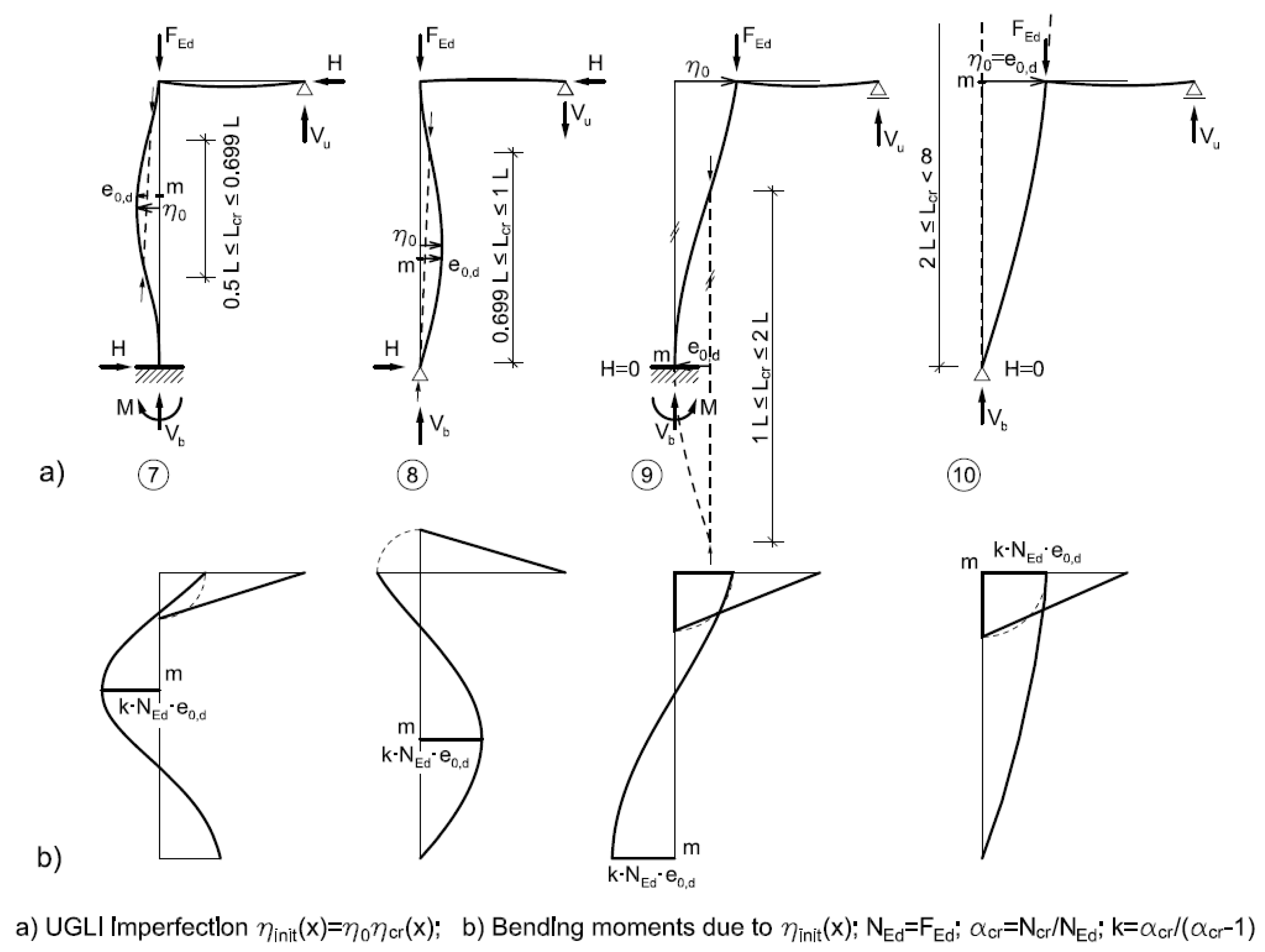
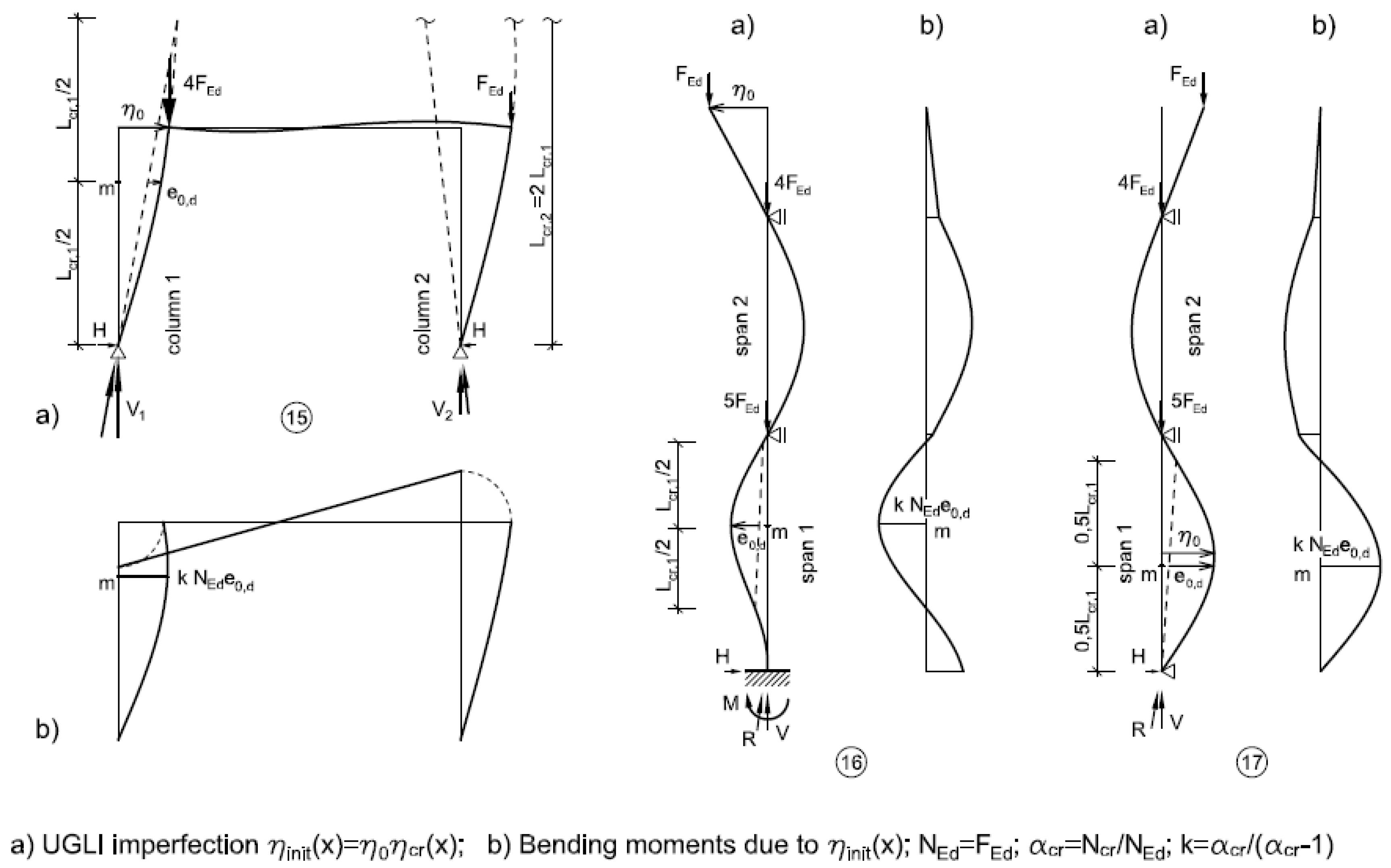
Geometrical interpretations are useful for practicing designers and for people from education institutes. Several examples are shown for the structures drawn in Figure 15, Figure 16, Figure 17 and Figure 18.

Figure 14. Geometrical interpretation of: (a) UGLI imperfection amplitude ${\eta }_0$ and (b) amplitude ${\eta }_{0,\mathrm{ad}}$ of the additional deformation of the member under study with length $L;$ (c) amplitude $e_{0,\mathrm{d}}$ of the equivalent member with length $L_{\mathrm{cr}}=0.699L$.

Figure 14. Geometrical interpretation of: (a) UGLI imperfection amplitude ${\eta }_0$ and (b) amplitude ${\eta }_{0,\mathrm{ad}}$ of the additional deformation of the member under study with length $L;$ (c) amplitude $e_{0,\mathrm{d}}$ of the equivalent member with length $L_{\mathrm{cr}}=0.699L$.

4. Amplitudes of the Equivalent Geometrical Imperfections according to Eurocodes [7,17]

The values of the initial local bow imperfection $e_0/L$ in the draft FprEN 1993-1-1:2021-11-26 [17] were changed compared to the current Eurocode EN 1993-1-1 [7].

According to 7.3.3.1 in [17], the equivalent bow imperfection, $e_0$, of the members for flexural buckling may be determined as follows:

$$e_0=\mathsf{\alpha }\beta \sqrt{\frac{f_{\mathrm{y}}}{235 \mathrm{MPa}}}L,$$

(74)

where the imperfection factor $\mathsf{\alpha }$ is in

Table 6. Design value of initial local bow imperfection $e_0/L$ according to 5.3.2b) in [7].

Buckling Curve, $\mathbf{Imperfection} \mathbf{Factor} \mathit{\alpha }$	Elastic Analysis	Plastic Analysis
	${\mathit{e}}_0/\mathit{L}$	${\mathit{e}}_0/\mathit{L}$
$a_0: \mathsf{\alpha }=0.13$	$1/350$	$1/300$
$a: \mathsf{\alpha }=0.21$	$1/300$	$1/250$
$b: \mathsf{\alpha }=0.34$	$1/250$	$1/200$
$c: \mathsf{\alpha }=0.49$	$1/200$	$1/150$
$d: \mathsf{\alpha }=0.76$	$1/150$	$1/100$

and $\beta$ is the relative bow imperfection according to

Table 7. Reference relative bow imperfection $\beta$ according to 7.3.3.1 in [17].

Buckling about Axis	Elastic Cross-Section Verification	Plastic Cross-Section Verification
$y-y$	$1/110$	$1/75$
$z-z$	$1/200$	$1/68$

.

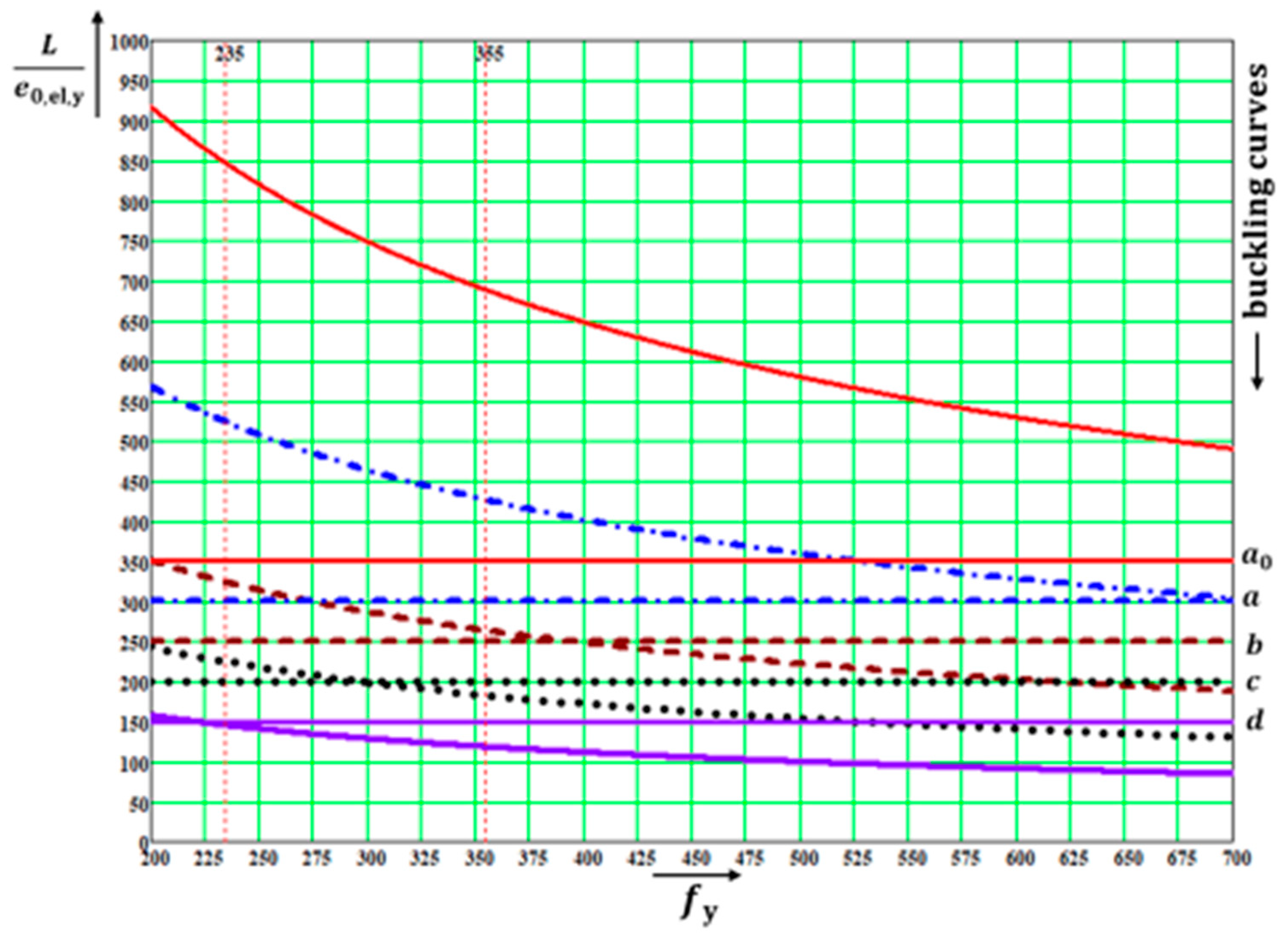
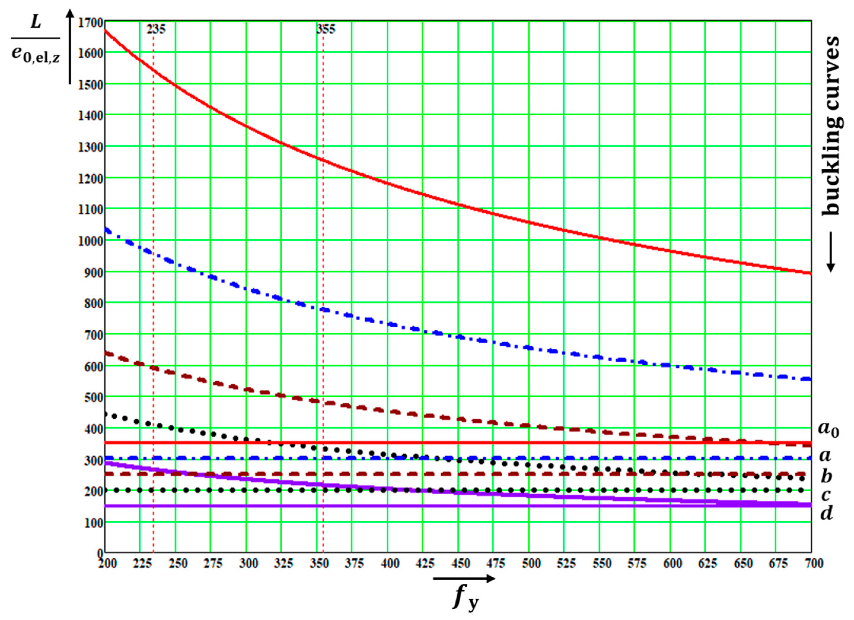
A comparison of the results in Figure 19 and Figure 20 to the values from Numerical Example 1 appears in

Table 8. Buckling about axis $y-y$. Comparison of bow imperfections $e_0$ for the second-order theory.

Numerical Example 1, Table 3		FprEN 1993-1-1:2021 [17]	EN 1993-1-1:2005 [7]
$e_{0,\mathrm{k}}$	$e_{0,\mathrm{d} }$	$e_{0,\mathrm{el},\mathrm{y}} \left(e_{0,\mathrm{pl},\mathrm{y}}\right)$	$e_{0,\mathrm{el},\mathrm{y}}$$\left(e_{0,\mathrm{pl},\mathrm{y}}\right)$
$14.92 \mathrm{mm}$	$15.63 \mathrm{mm}$	$22.9, \left(33.6\right) \mathrm{mm}$	$40, \left(48\right) \mathrm{mm}$

for buckling about axis $y-y$ and in

Table 9. Buckling about axis $z-z$. Comparison of values $e_{0, } M_{\mathrm{Ed},\mathrm{c}}^{\mathrm{II}}, U^{\mathrm{II}} \mathrm{and} \left(U_{\mathrm{MN}}\right)$ of the second-order analysis.

Numerical Example 1, Table 4		FprEN 1993-1-1:2021 [17]	EN 1993-1-1:2005 [7]
$e_{0,\mathrm{k}}$	$e_{0,\mathrm{d} }$	$e_{0,\mathrm{el},\mathrm{z}} \left(e_{0,\mathrm{pl},\mathrm{z}}\right)$	$e_{0,\mathrm{el},\mathrm{z}}\left(e_{0,\mathrm{pl},\mathrm{z}}\right)$
$8.09 \mathrm{mm}$	$10.51 \mathrm{mm}$	$18.55, \left(27.2\right) \mathrm{mm}$	$24, \left(30\right) \mathrm{mm}$
$M_{\mathrm{Ed},\mathrm{c}}^{\mathrm{II}}$ calculated by FE-STAB [1] $\mathrm{for} N_{\mathrm{Ed}}=859.584 \mathrm{kN},$$\mathrm{for} \mathrm{the} \mathrm{above} e_0$$\mathrm{values} \mathrm{with} {\gamma }_{\mathrm{M}1}=1.1$
$22.96 \mathrm{kNm}$	$29.83 \mathrm{kNm}$	$52.65 \mathrm{kNm}$	$68.12 \mathrm{kNm}$
$U^{\mathrm{II}}; \left(U_{\mathrm{MN}}\right), U_{\mathrm{N}}=0.348$
$0.85; \left(0.502\right)$	$1.0; \left(0.652\right)$	$1.499; \left(1.151\right)$	$1.837; \left(1.489\right)$
$N_{\mathrm{Ed}}$$\mathrm{to} \mathrm{obtain} U^{\mathrm{II}}=1.1$
$916 \mathrm{kN}$	$N_{\mathrm{Ed}}=N_{\mathrm{b},\mathrm{Rd}}$ $=859.584 \mathrm{kN}$	$723 \mathrm{kN}$	$656 \mathrm{kN}$

for buckling about axis $z-z$.

It is evident in the UGLI imperfection method that safety factor ${\gamma }_{\mathrm{M}1}$ cannot be removed from $e_{0,\mathrm{d}, }$ and value $e_{0,\mathrm{k}}$ cannot be used in this method. See comparisons in Table 8 and Table 9.

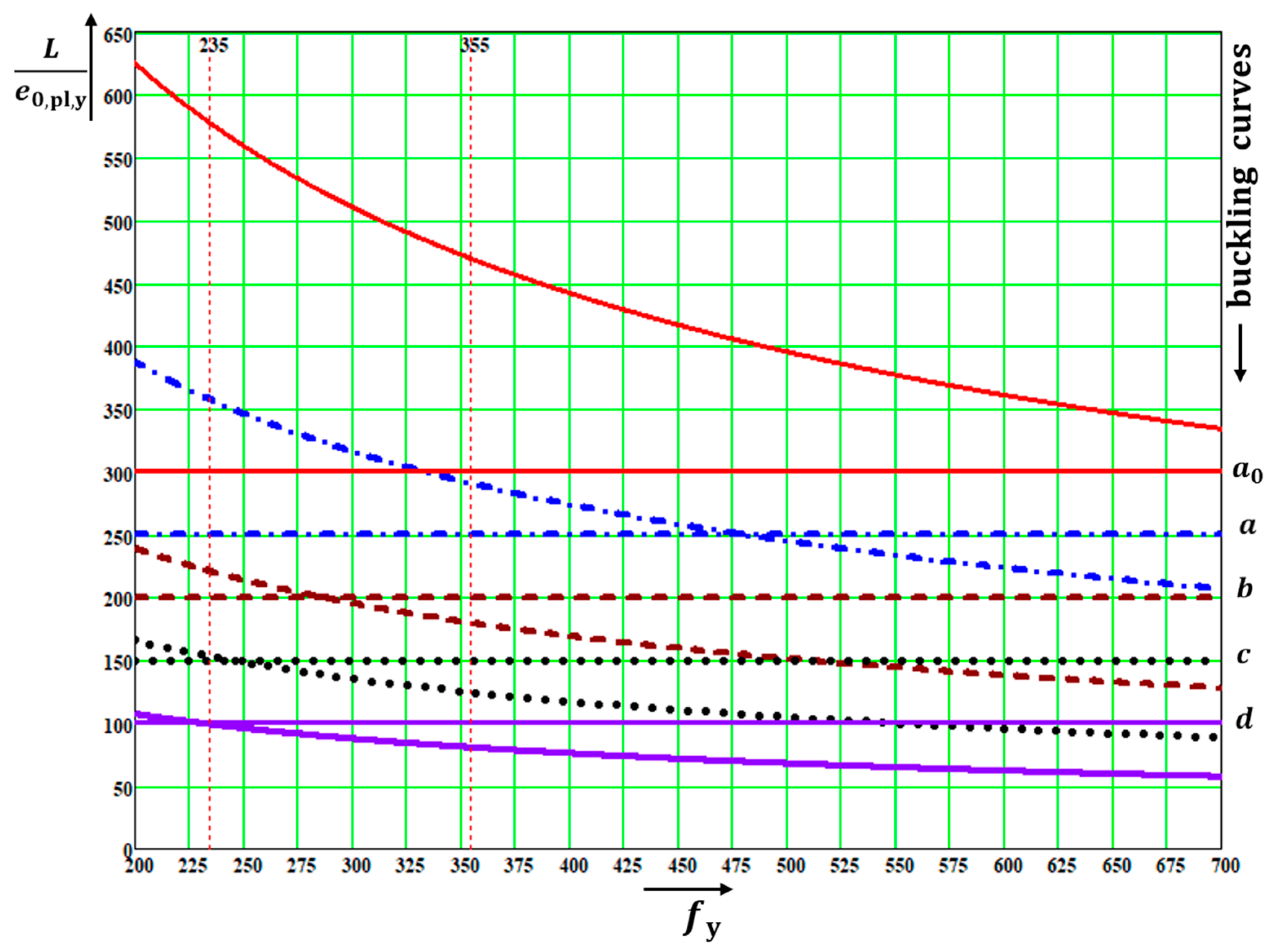
From the comparisons in the above diagrams in Figure 19, Figure 20, Figure 21 and Figure 22 for the values of bow imperfections $e_0$ used in the second-order theory, the results read as so:

The $e_0$ values for the plastic cross-section verification were higher than those for the elastic ones, $e_{0,\mathrm{pl}}>e_{0,\mathrm{el}}$;

The $e_0$ values for the buckling about the axis $y-y$ were higher than those for the buckling about the axis $z-z$, $e_{0,\mathrm{y}}>e_{0,\mathrm{z}}$;

If $e_{0,\mathrm{d}}$ was used in the second-order theory, identical results were obtained to the EM method in the ultimate state when $N_{\mathrm{Ed}}=N_{\mathrm{b},\mathrm{Rd}}.$ The UGLI imperfection method is based on this fact. It has long since been known that the current Eurocode [7] prescribes in 5.3.2b) much higher $e_0$ values than those accepted in the EM method. See, for example, the parametrical study in [21]. This could be the reason why in draft [17], the new $e_0$ values for almost all the combinations were lowered. The dramatic drop in the $e_0$ values was seen for the imperfection factor of buckling curve $a_0$.

$e_0$, according to draft Eurocode [17], also depends on the yield strength $f_{\mathrm{y}}$. Generally, the new way to calculate $e_0$ according to [17] gives lower $e_0$ values compared to those given in the current Eurocode [7]. This is valid for: all the $e_{0,\mathrm{el},\mathrm{z}}$ values (Figure 19); the $e_{0,\mathrm{el},\mathrm{y}}$ values with the imperfection factors $a_0,a$; and $e_{0,\mathrm{pl},\mathrm{y}},e_{0,\mathrm{pl},\mathrm{z}}$ with the imperfection factor $a.$ It is also valid for $f_{\mathrm{y}}\le 235 \mathrm{MPa},$ except the cases for $e_{0,\mathrm{pl},\mathrm{z}}$ with the imperfection factors $c \mathrm{and} d$.

The lower $e_0$ values in draft [17] are still higher than the $e_{0,\mathrm{d}}$ values used in the UGLI imperfection method. Therefore, $e_{0,\mathrm{d}}$ must not be lowered by removing ${\gamma }_{\mathrm{M}1}$ from Equation (19) to obtain (8).

5. Conclusions

The second-order theory was used to analyze the flexural buckling of an individual member simply supported on both member ends, with a uniform double symmetric cross-section under uniform axial compressed force in an elastic state. It is well known that the equivalent member (EM) method is actually the modified second-order theory with a “hidden” amplitude $e_{0,\mathrm{k}}$ (8) of the equivalent geometrical initial imperfection, which has the shape of the elastic critical buckling mode (9).

This paper aims to show that under condition $N_{\mathrm{Ed}}=N_{\mathrm{b},\mathrm{Rd}}$ (utilization factor $=N_{\mathrm{Ed}}/N_{\mathrm{b},\mathrm{Rd}}=1.0$):

(a) the same utilization factor $U_{\mathrm{EMM}}=N_{\mathrm{Ed}}/N_{\mathrm{b},\mathrm{Rd}}=1.0$ value, given by the EM method (33), can also be given by the second-order theory from Equation (34), $U^{\mathrm{II}}=U_{\mathrm{N}}+U_{\mathrm{M}}=0.88+0.12=1.0,$ if the amplitude $e_{0,\mathrm{d}}$ (19) is used in the calculation; (b) the same utilization factor $U=1.0$ can also be obtained by the UGLI imperfection method if the design value of the imperfection amplitude $e_{0,\mathrm{d}}$ (19) is used in the calculation. It is very important to state that safety factor ${\gamma }_{\mathrm{M}1}$ must not be removed from $e_{0,\mathrm{d}}$, which was mistakenly performed in [17], where $e_{0,\mathrm{d}}$ (19) was replaced with $e_{0,\mathrm{k}}$ (8). In [7,8,16], the correct value $e_{0,\mathrm{d}}$ (19) was used in the UGLI imperfection method, as it was prescribed by its authors Chladný and Baláž in their publications [10,11,12,13,14,15,18,19]. Using $e_{0,\mathrm{k}}$ (8) in the UGLI imperfection method, which was incorrectly recommended in [17], leads to member resistances (and also to utility factors $U$) on the unsafe side, especially for very slender columns; e.g., for a relative slenderness $\overline{\mathsf{\lambda }}=2.0$, the difference between utility factors $U^{\mathrm{II}}=U_{e_{0,\mathrm{d}}}^{\mathrm{II}}$ and $U_{e_{0,\mathrm{k}}}^{\mathrm{II}}$ is 41% on the unsafe side (see Figure 4). The above facts are illustrated in Numerical Example 1.

Chapter 3 informs about: (a) unknown details from historical developments of the UGLI imperfection method invented by Chladný [10,11]; (b) the best version of the UGLI imperfection method by Chladný and Baláž, which is found in [16]; and (c) illustrative Numerical Example 2, in which the column fixed at one end and simply supported on the other end was investigated. The purpose was to show that amplitudes have a geometrical interpretation (Figure 14) for the member with a uniform cross-section and uniform axial force distribution, as previously described by Baláž in [12,18]. This invention is very important because it enables the following without almost any calculation: (a) estimating the buckling length $L_{\mathrm{cr}};$ (b) determining the location of the amplitude $e_{0,\mathrm{d}}$, which is always in the middle of $L_{\mathrm{cr}};$ and (c) calculating the maximum bending moment due to the axial compressed force $N_{\mathrm{Ed}}$ acting on the member with the equivalent geometrical imperfection from the simple formula $M_{\mathrm{Ed}}^{\mathrm{II}}=k{M}_{\mathrm{Ed}}^{\mathrm{I}}=k{N}_{\mathrm{Ed}}{e}_{0,\mathrm{d}}.$ The maximum bending moment $k{N}_{\mathrm{Ed}}{e}_{0,\mathrm{d}}$ is located at the same point $m$, where the amplitude $e_{0,\mathrm{d}}$ is also located. All these details, together with the shapes of the equivalent geometrical initial imperfections (46) and bending moment distributions, appear in Figure 15, Figure 16 and Figure 17 for 17 cases. In Numerical Example 2, the hand calculation results were verified by the results of the computer program IQ 100 [20]. A perfect agreement was achieved.

This paper shows, for the first time ever, that: (a) the curve valid for the ideal member can be added to the five buckling curves if the imperfection factor $\alpha =0$ value is used in the Formula (15) that is valid for the reduction factor $\chi$, and (b) of the four quantities $\chi , \overline{\lambda }, \alpha , \mathrm{and} {\overline{\lambda }}_0$ used for drawing the five buckling curves, it is possible, together with safety factor ${\gamma }_{\mathrm{M}1,}$ to obtain plenty of other information. For the following dimensionless quantities, values can be easily calculated and their distributions can also be drawn for ${\alpha }_{\mathrm{cr}},\left(23\right),k,\left(24\right),e_{0,\mathrm{k}}/j,e_{0,\mathrm{d}}/j,\left(20\right),{\eta }_{\mathrm{tot},\mathrm{c},e_{0,\mathrm{k}}}/j,{\eta }_{\mathrm{tot},\mathrm{c}}/j,\left(30\right),U_{\mathrm{N}},\left(31\right),U_{\mathrm{M}},\left(31\right),U_{\mathrm{M},e_{0,\mathrm{k}}},\left(37\right),$$U^{\mathrm{II}},\left(32\right), \mathrm{and} U_{e_{0,\mathrm{k}}}^{\mathrm{II}},\left(38\right).$ Consequently, after multiplying relative dimensionless amplitudes by the factor $j=W/A$, the values of several amplitudes can also be given: $e_{0,\mathrm{k}}, e_{0,\mathrm{d}}, {\eta }_{\mathrm{tot},\mathrm{c},e_{0,\mathrm{k}}}, \mathrm{and} {\eta }_{\mathrm{tot},\mathrm{c}},$ as can the characteristic and design values of the amplitudes of the additive deformations ${\eta }_{\mathrm{ad},\mathrm{d},\mathrm{c},e_{0,\mathrm{k}}} \left(35\right) \mathrm{and} {\eta }_{\mathrm{ad},\mathrm{d},\mathrm{c}},$ which are the differences between the values of the amplitudes of the total and initial deformations.

The geometrical interpretations of the distributions of all these quantities appear in Figure 4, Figure 5, Figure 6, Figure 7, Figure 8, Figure 9, Figure 10, Figure 11, Figure 12 and Figure 13. These diagrams are very useful for practicing designers, educators, and university students.

The comparisons of the amplitudes of the equivalent geometrical imperfections according to Eurocodes [7,17], used for the elastic and plastic cross-section analyses when applying the second-order theory, are given in Section 4. The comparisons are presented in a convenient graphical form in Figure 19, Figure 20, Figure 21 and Figure 22. The results from the detailed analysis of the comparisons are summarized in Figure 22 immediately before Section 5. The conclusions are, therefore, not repeated here. Nevertheless, it must be underlined that the lower $e_0$ values (74) taken from the draft [17] when comparing with values given in Table 6 [16] were still higher than the $e_{0,\mathrm{d}}$ values used in the UGLI imperfection method. This provides further evidence that $e_{0,\mathrm{d}}$ must not be replaced with a lower $e_{0,\mathrm{k}}$ value. In other words, safety factor ${\gamma }_{\mathrm{M}1}$ must not be removed from the Formula (19) defining $e_{0,\mathrm{d}}$, which was incorrectly performed in [17].

Mandate M/515 for amending the existing Eurocodes and extending the scope of structural Eurocode includes the following requirement: wherever possible, metal Eurocodes (EN 1993 for steel structures and EN 1999 for structures from aluminum alloys) should unify procedures. The clause about the UGLI imperfection method in [16] is correct, but is incorrect in [17]. Draft [17] must be corrected.

The UGLI imperfection method is a very promising and effective method that can be applied to many types of building and bridge structures [14,15,18], and also to large arch bridges [19]. The UGLI imperfection method must be modified for the rib of basket handle arch-type bridges. This has been accomplished by Chladný in the Slovak National Annex [9], and has been used for the Apollo bridge design over the Danube in Bratislava in the Slovak Republic and for the Pentele bridge design over the Danube between Dunaújváros and Dunavecse in Hungary [14,15]. Baláž used the UGLI imperfection method for the Žďákov bridge [19] designed by Josef Zeman (*1922–†1997) and opened in 1967, with its span of 330 m becoming the world record in its category. The UGLI imperfection method is not applicable for plated structural elements or shells.