Abstract
The article presents the results of an analysis of the surface roughness parameters, microhardness, and the stresses of the surface layer ofFSW butt joints subjected to the burnishing process with a diamond tip. This can be useful in selecting the optimal parameters of the burnishing process, ensuring the best properties of the surface layer of the FSW joint. Burnishing force and feed rate influence were analyzed according to the two-factor three-level full factorial statistical completed plan PS/DC 32. The tested material was 2024-T3 aluminum alloy sheets with a thickness of 2 mm. The results show that burnishing significantly reduced the surface roughness from Sa = 6.46 μm to Sa in the range of 0.33 μm–1.7 μm. This treatment provides high compressive residual stresses from −86 to −130 MPa and from −158 to −242 MPa. Microhardness increased from 84.19% to 174.53% compared to butt joints. Based on the obtained results, multi-criteria optimization was carried out. This optimization allows us to obtain a compromise solution ensuring compressive stresses in the surface layer ( and ) and microhardness with the roughness of the weld surface Sa = 0.28 µm, Sku = 3.93 and Spc = 35.88 1/mm.
1. Introduction
The trend of lightweight construction in applications such as aerospace, railway, and automotive [1] has included new joining technologies (Friction stir welding [1,2], Laser beam welding [3], Refill friction stir welding [4], Pinless friction stir spot welding [5], adhesive joints [6]) and new materials (high strength steels, aluminum, magnesium and titanium alloys). The Friction Stir Welding (FSW) technology is used, among others, on non-weldable aluminum alloys, as the process does not involve melting and, therefore, cannot solidify [7]. Other benefits associated with this process are higher weld quality compared to traditional arc welding techniques [8], repeatability of welding parameters, low environmental impact in terms of gas generation, simple equipment requiring relatively low levels of operator training, refurbishment of damaged components previously considered uneconomical [9]. Joints obtained by this method reduce costs by up to 30% and weight reduction by 10% compared to the mechanical joining technique [10]. In joints made by the FSW method, as well as in other conventional welding processes, the weakest point in terms of fatigue strength is the welded joint [11].This is related to the introduction of tensile residual stresses at the weld zone.
Burnishing is one of the methods that has a beneficial effect on the strengthening of the surface layer [12,13]. It includes methods such as slide diamond burnishing (SDB) [14], ball burnishing (BB) [15,16], roller burnishing (RB) [17], or shot peening (SP) [18]. In the case of slide burnishing, tooltips are usually made of small-sized diamond composites. The small contact surface of the tool with the workpiece necessary for plastic deformation is smaller than in other burnishing methods. This, in turn, enables the strengthening of thin-walled elements such as FSW welded joints [19]. By using slide burnishing, we can obtain good surface smoothness, improve hardness and introduce compressive stresses in the top layer [20]. These features have a positive effect on fatigue strength [12,14], corrosion resistance [21], or tribological wear [22,23]. Zielecki et al. [12] applied slide burnishing to improve the fatigue strength of shoulder fillets of the shaft made of X19NiCrMo4 steel. The slide burnishing process improved the fatigue strength by 28.5%, reduced the surface roughness Ra in the range from 64.1% to 85.8%, and strengthened the surface layer by 32% down to a depth of 0.018 mm compared to the hardness of the core. Korzynski et al. [14] studied the effect of SDB on the fatigue strength of chromium-coated elements made of 42CrMo4 alloy steel. They indicate that after burnishing, the fatigue strength of shafts can be improved by up to 40%. In work [21], authors analyzed the influence of drawing, polishing, and slide diamond burnishing on the corrosion resistance of 1.4571 stainless steel. Based on microscopic observations, they found that the best corrosion resistance was found after burnishing. Nestler and Schuber [24] examined the SDB of aluminum matrix composites. The results demonstrate that this treatment significantly reduces the value of surface roughness and imperfections such as voids. They also indicated that the burnishing feed has the greatest influence on surface roughness.
In the literature, only a few articles were found on the application of the burnishing process in elements welded using the FSW method. In works [25,26],the authors investigated the influence of the ball-burnishing process on the mechanical properties of 2050 Al alloy using different burnishing configurations. They found that the ball-burnishing treatment of FSW joints increased the hardness in the range of 10–40% and generated compressive residual stresses from −315 MPa to −700 Mpa.
Statistical methods Design of Experiments (DoE) allows one to conduct an experiment and obtain results often impossible to obtain in any other way or require much higher costs [27]. In articles and studies on the subject of burnishing, DoE is often used to indicate the optimal process parameters in the tested parameter range. Due to the complexity of modern processes, the use of classical methods of planning an experiment may not bring the expected results. Therefore, the research methodology is often supported with an analysis using artificial neural networks and multi-criteria optimization. Authors of work [28] investigated the influence of slide burnishing of shafts made of heat-treated steel 42CrMo4 on their surface roughness using the Hartley plan and artificial neural networks. The results obtained with the neural model indicate a relationship in which an increase in the burnishing force results in a decrease in the roughness of the shaft surface. They also observed that the feed rate during burnishing has a significant effect on the Ra roughness. A low feed rate with a low burnishing speed leads to a small Ra parameter, while a high feed rate at the same burnishing speed results in the highest values of roughness. In turn, Kubit et al. [2] used the Design of Experiments and multi-criteria optimization to point out appropriate parameters of the FSW process for EN AW-2024-T3 Al alloy. They concluded that an increase in the welding speed at a given value of pin length caused a decrease in the load capacity of the joint and a significant increase in the dispersion of the results.
Therefore, research into the search for the best variants of the burnishing process of welded joints with the FSW method is justified. The article presents the study of the effect of selected parameters of static burnishing on the properties of a surface layer of FSW butt joints. A two-factor three-level full factorial Design of Experiments plan (DoE) was used to model the relationship between burnishing force and feed rate on the residual stresses, roughness, and microhardness. Based on the results of the residual stresses in two directions (σx, σy), roughness parameters (Sa, Sku, Spc) and microhardness (HV) of the FSW joint, multi-criteria optimization was carried out to indicate the appropriate parameters of the burnishing process.
2. Materials and Methods
2.1. Material
In the present article, high-strength aluminum alloy EN AW-2024-T3 [29], with a thickness of 2 mm, was selected to investigate the effect of slide diamond burnishing on residual stress, surface roughness, and microhardness joints welded with the FSW method. The chemical composition of this alloy is presented in Table 1, and the mechanical properties are in Table 2. This type of aluminum has various applications, including in aviation, automotive or military industries [30].

Table 1.
Chemical composition of the EN AW-2024-T3 aluminum alloy (wt.%) [31].
Table 2.
Mechanical properties of the EN AW-2024-T3 aluminum alloy [31].
2.2. Method
Two strips with dimensions 400 mm (length) × 100 mm (width) × 2 mm (thickness) were butt welded using the friction stir welding method on a universal vertical milling machine Jafo FWF 32J2 (Figure 1). The welding process was carried out with the following parameters: rotational speed n = 1100 rpm, feed rate f = 80 mm/min, the plunging depth of the pin was set to 85% (d = 1.7 mm) of the sheet thickness in turn the shoulder penetration was set to 2.5%, inclination angle of the tool of 3°.
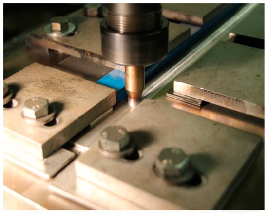
Figure 1.
Friction stir welding process.
The slide diamond burnishing was performed on a vertical CNC milling machine VF-1 (HaasAutomation Inc., Oxnard, CA, USA).The SDB process was carried out on a test stand (Figure 2a) using a DB-3 burnishing tool (Figure 2b, Cogsdill-Nuneaton Ltd., Nuneaton, UK). This article used a tooltip made of polycrystalline diamond.
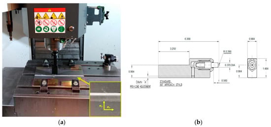
Figure 2.
Slide diamond burnishing process (a) and burnishing tool (b).
The experimental investigations were carried out in accordance with the two-factor three-level full factorial design of experiments PS/DC 32. The input parameters include the force burnishing P and feed rate f (Table 3).
Table 3.
The burnishing parameters used in research according to PS/DC 32.
Residual stresses in the surface layer were performed by X-ray diffraction analysis using a Proto iXRD Combo and computer software XRD Win 2.0 from Proto Manufacturing (Taylor, MI, USA). The measurements were made with a chromium anode using the sin 2Ψ method [32] at a diffraction angle (2θ = 139.3°) in the range of 25° to 25°. Measurements were made in two directions: longitudinal (σy) and transverse (σx) on the joint surface before and after burnishing (Figure 2a). The roughness tests were performed using the Talysurf CCI L5xZ1B1S1F5Hpk scanning interferometer from Taylor Hobson (Taylor Hobson Ltd., Leicester, UK). The measurement area was 3.3 mm × 3.3 mm. Points not measured were filled using the “smooth shape” method calculated on the basis of neighbors. A third-degree polynomial was used to remove the curvature. All measured parameters in the 3D system were measured in accordance with the applicable standard PN-EN ISO 25178-2:2022-06 [33].
The selection of the regression function was carried out using the principle of least squares in the following form of the criterion evaluating the quality of the approximation (1):
where the value of the R function is a measure of the deviation of the approximating function W(x) from the approximated f(x), i = 1, …, N—number of experiments.
To describe the process, the form of an algebraic polynomial of degree m was adopted, containing the interactions between the process parameters:
where there are L unknown coefficients , , , , , , with i, j, …, n = 1, …, S—variables of the polynomial (2) and .
The Fisher–Senecor test was used to assess the adequacy of the regression equation with the test results. At the first stage of the analysis, the adequacy variance was determined (3):
where —mean value of the measurement results in the i-th experiment, —value calculated from the regression equation for the levels of the input and output factors of the i-th experiment, k—the number of terms of the regression equation (without the intercept) after discarding irrelevant terms.
Then, the value of the test factor was determined F(4):
and compared with the critical value determined from the Fisher–Snedecor distribution tables.
3. Results and Discussion
3.1. Residual Stress
This process of welding aluminum alloys enables the production of aircraft structures while reducing labor consumption, costs, and weight, while maintaining comparable or higher strength parameters compared to conventional joining methods. However, it introduces tensile stresses in the joint. Tensile stresses improve dislocation mobility and, as a result, reduce hardness [34,35]. Plastic deformation occurring in the surface layer of the weld under the influence of the burnishing tool with a diamond tip can be considered a process of generating new dislocations and their displacement. Dislocationgeneration occurs when a certain level of stress is reached. Since the deeper, non-deformed layers do not change, compressive stresses arise in the surface layer of the joint, increasing the joint’s fatigue strength.
Figure 3 and Table 4 present the results of measurements of residual stresses of butt joints subjected to slide burnishing with a diamond tool. The analysis of the test results shows that, regardless of the adopted setting parameters of the process, slide burnishing introduces compressive stresses both in the direction transverse to the weld axis and along the weld axis ( direction). In the x-axis direction, the largest increase in compressive stresses from to was recorded for experimental run no. 4 ( and ). In turn, in the direction of the y-axis, as a result of applying a force of and a feed rate of (experimental run no. 7), compressive stresses of were introduced. It should be noted that before the burnishing treatment in the considered direction, only small compressive stresses of .
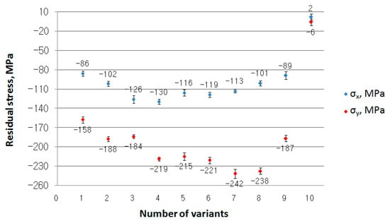
Figure 3.
Residual stress of the EN AW-2024-T3 butt welded joints after SDB.
Table 4.
The results of residual stresses according to PS/DC 32.
For stresses in the transverse direction, at feed rates of and , an increase in contact force causes an initial increase in compressive stress by 51.16% at a feed rate of and 13.75% at a feed rate of , and next decrease in compressive stress (Figure 4a). In the case of a , the highest value of compressive stresses was recorded at a burnishing force of . In this case, a further increase in the burnishing force causes only a decrease in the stress value. In the case of stresses in the longitudinal direction, the opposite trend can be observed. At the feed rate of and , the increase in the tool clamping force causes an increase in the value of compressive stresses. In the case of the feed rate of , as a result of changing the force from to , the compressive stress increased by 53.16% (to ), while at the feed rate of by 26.59% to the value of ). At the feed rate , the increase in force from to initially results in an increase in the compressive stress value by 20.10% to , and then with the increase in force, a decrease in the stress value by 13.38% (Figure 4b).
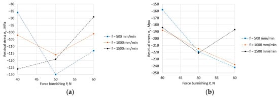
Figure 4.
Influence of feed rate and force burnishing on residual stress value (a) in the transverse direction , (b) in the longitudinal direction .
Table 5 presents the results of the significance analysis (ANOVA test—p-value) of the impact and on and
Table 5.
The p-value for ANOVA test— and .
The results show that is statistically significant (p = 0.047) for .
Based on the ANOVA analysis of variance, an adequate stress value regression model was developed at the significance level in the transverse direction (5) (Figure 5a):
and in the longitudinal direction (6) (Figure 5b):
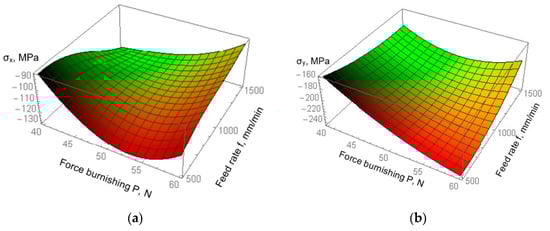
Figure 5.
Plots of the regression functions of residual stresses (a) in the transverse direction , (b) in the longitudinal direction .
Table 6 presents the R2 (coefficient of determination) value and significance analysis (p-value) for individual structural elements of regression models for and . The R2 value shows the high accuracy of the models. Moreover, the results indicate that not all structural elements of the model are statistically significant. However, attempts to omit them in the model resulted in a decrease in the quality of the model—a decrease in the value of R2.
Table 6.
R2 value and p-value for individual structural elements of regression models.
3.2. Surface Roughness
Table 7 presents the results of surface roughness for the specimen after FSW (base variant) and after SDB according to PS/DC 32 plan. Selected roughness parameters such as Height parameters, Spatial parameters, Hybrid parameters, Feature parameters, and Functional parameters were analyzed.
Table 7.
Results of surface roughness of the EN AW-2024-T3 aluminum alloy burnished using a diamond tool.
The base surface was characterized by a relatively high value of the height parameters of the surface. The average arithmetical mean height of the surface Sa was 6.46 µm (Figure 6a). The largest maximum height of the surface Sz was 42.5 µm, which consisted of the maximum height of peaks Sp = 18.8 µm and the maximum height of valleys Sv = 23.7 µm. The surface was also characterized by a slight skewness (Ssk = 0.592), and a negative value of this coefficient indicates a surface with plateau hills.
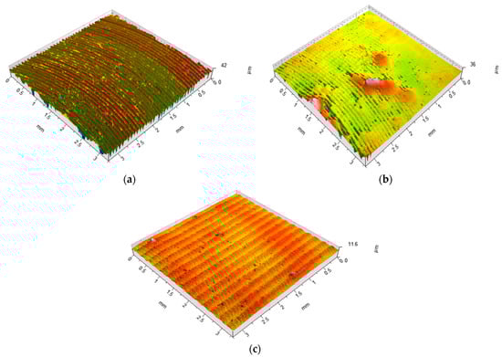
Figure 6.
Isometric views (a) of the base surface and the SDB surfaces: (b) , (experimental run no. 2), (c) , (experimental run no. 8).
The kurtosis of height distribution Sku, defined as a measure of the probability density of the height of the surface roughness, was 2.32. This parameter is most often a measure of the number of sharp and high peaks or sharp and deep valleys (e.g., scratches or surface scratches). For a perfectly random surface, the Sku parameter takes a value of 3. Values lower than 3 indicate less steep areas of the surface. As a result of the SDB, a clear reduction in the height parameters of the surface was obtained. The parameter Sa was in the range of 0.333–1.7 µm, and the parameter Szwas in the range of 5.86–36.1 µm. A similar reduction of parameters was also obtained in the case of Sp, Sv, and the feature parameters such as S10z, S5p, and S5v. It is worth noting that particularly high values of Sa and Sz parameters were expressed in specimens 2 and 3, burnished with the lowest value of the burnishing force P = 40 N. The analysis of the geometric surface structure showed that burnished surfaces with a force of P = 40 N contained numerous surface defects as a result of the burnishing process.
The increase in the value of the burnishing force to P = 60 N resulted in the elimination of this unfavorable phenomenon. The scatter of Ssk and Sku parameters of the burnished surfaces was quite large and ranged from −0.813 (experimental run no. 1) to 1.07 (experimental run no. 4) for Ssk. For Sku, it ranged from 2.59 (experimental run no. 7) to 11.7 (experimental run no. 8). The unfavorable impact of the lowest burnishing force value is also evidenced by the fact that individual values of the spatial parameter Str (texture aspect ratio of the surface) were obtained. This parameter expresses the relationship between the shortest and longest decay of the correlation function and takes values in the range of 0–1. Values close to 1 indicate that the GSS has a high level of isotropy, and values close to 0 characterize anisotropic surfaces (Figure 7). The sliding burnishing process is usually characterized by anisotropicity of the obtained surfaces, which was confirmed in the case of specimens 6–9. On the other hand, the Str value for specimens 1–5 places them in the range of mixed textures or, as in the case of specimen 3, close to random surfaces.
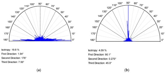
Figure 7.
Isotropic rose (a) for the base variant and (b) after burnishing , (experimental run no. 8).
The Sal auto-correlation length is the shortest segment over which the normalized auto-correlation function decreases to a value τ which is greater than or equal to zero and less than 1. Large values of the spatial parameter Sal mean that the surface is dominated by low-frequency components, while a small value of Sal is the reverse case. For the base surface, the parameter Sal was 0.021 mm and was clearly lower than in the case of specimens 1–6 (0.2–0.25) and slightly lower than in the case of specimens with the highest feed value 7–9 (0.07–0.08). The developed interfacial area ratio Sdr is defined as the ratio of the increment of the boundary area in the area of definition to the size of the area of definition. This parameter is used as a measure of surface complexity, especially when comparing surface conditions between treatments. In the case of a real flat surface, Sdr = 0, and parameter values less than 1% are characteristic of smoothness finishing treatments, such as honing, lapping, polishing, etc. Burnishing treatment allowed us to obtain Sdr parameter values below 1%, i.e., typical for smoothness treatments. Moreover, values below 0.1% were obtained for specimens for which the force burnishing was and .
Another hybrid parameter—the root mean square gradient of the surface Sdq is calculated as the root mean square slope of all points in the defined area. The Sdq of a completely flat surface is 0. This parameter can be, for example, used to evaluate surfaces in sealing applications and to differentiate surfaces with a similar value to the Sa parameter. In the case of the base surface, the value of the Sdq parameter was 0.64, with Sdq = 0.2 for burnished surfaces. The lowest values of the Sdq parameter, similarly to Str, were obtained for specimens for which the force burnishing was and . Lower values of the Sdq parameter in the case of burnished surfaces indicate a more smooth surface.
The bearing area curve (BAC) (Abbott–Firestone curve (AFC)) is a kind of description of the differentiation of surface properties changing with its depth (Figure 8). The curve is divided into parts related to summits, cores, and valleys, thanks to which it is possible to calculate the reduced summit height Spk, the height of the core Sk, the reduced valley depth Svk and two values of the material contribution Smr1 (upper bearing area) and Smr2 (lower bearning area). Large Spk values characterize a surface consisting mostly of high summits providing a small initial contact area and, thus, high contact stress values when the surfaces are in contact. Sk can be used as a measure of the effective roughness depth after the initial running-in period. The Svk parameter, on the other hand, is a measure of the fluid-holding capacity of the sliding surfaces. Surfaces that require good lubrication should have high Svk values. Spk was lower than Svk in all analyzed cases, including the base specimen. Such a value of peaks leads to minimization of the lapping allowance provided for in operation and may indicate better tribological properties of the surface. On the other hand, increasing the Spk value leads to a decrease in the actual contact area, which may limit the impact of adhesive interactions.
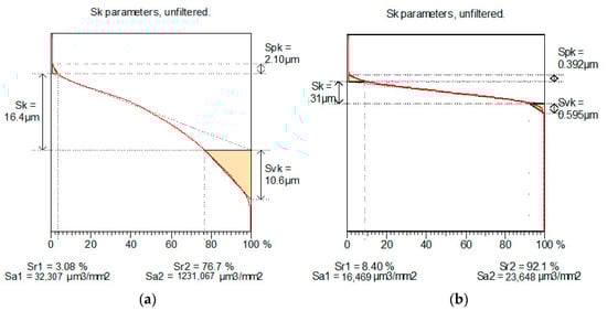
Figure 8.
Abbott–Firestone curve (a) for base surface and (b) after burnishing , (experimental run no. 8).
Additional data on fluid retention in microgroove valleys at the interface of mating surfaces, valuable for constructors, can be obtained on the basis of vectorization of the microgroove network. The characteristic networks of microgrooves for the base and burnished surfaces are shown in Figure 9. The TalyMap 6.0 software allows us to determine three important parameters: the maximum and average depth of the grooves and their density. The maximum depth of grooves for the base surface, which is 31.5 μm, is significantly greater than for burnished surfaces (2.84–6.21 μm). In turn, the density of the grooves after the burnishing process was relatively similar to the density of the grooves after the treatment of the base specimen (212–284 cm/cm2). The surface structure can also be assessed on the basis of the vector distribution of microgrooves. In the case of the burnished surface (experimental run no.9), these observations only confirm the earlier observations regarding the anisotropic structure.
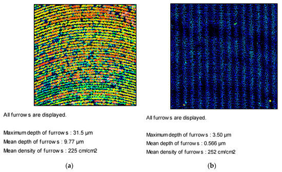
Figure 9.
Vectorization of the microgroove network (a) for base surface and (b) after burnishing , (experimental run no. 9).
The density of peaks Spd is a parameter included in the group of features. It expresses the number of elevations per unit area. The Spd parameter determines the density of bumps on the tested surface. In the case of the base surface, the value of the Spd parameter was 45.9 1/mm2. The burnishing process reduced this parameter. Only in experimental run no. 7, it increased slightly to Spd = 52.2 1/mm2. In other cases, it ranged from 1.93 to 30.7 1/mm2.
The arithmetic mean peak curvature Spc is another parameter from the group of features. A smaller value of the parameter indicates that the tops of the surface are characterized by rounded shapes, while higher values indicate their “sharp” character. Depending on the value of the Spc parameter, various types of surface deformation may occur, such as elastic, elastic-plastic, and plastic. For the base specimen, the Spc parameter reached a value of 59.3 1/mm. This parameter increased for specimens where the burnishing force was P = 40 N. In other cases, the peaks of the burnished surfaces had a more rounded shape than the base specimen. The lowest value of the parameter Spc = 28.5 1/mm was obtained for experimental run no. 7, which was also characterized by the highest density of vertices.
Based on the obtained test results, it can be concluded that the smallest value of the burnishing force , although it contributes to the reduction of height parameters compared to the base specimen, at the same time causes a number of surface damages in the form of furrows, scratches, and build-up. The situation is much better in the case of the other two force values, i.e., and . The reduction of the height of irregularities is then clear and stable (Sa in the range of 0.333 μm–0.666 μm). However, it can be noticed that the maximum smoothing of the surface was obtained in variants 6 and 9 (0.333 μm and 0.359 μm), i.e., corresponding to the force of and and the highest feed rate . It seems that the use of input parameters at the mentioned levels will ensure obtaining optimal GSS results.
Due to the fact that there is a high statistical correlation between some roughness parameters, only the parameters carrying the most information about the process were adopted for the analysis of optimization of burnishing process parameters. In the case of height parameters between the parameters Sa, Sz, Sv, Sp, and Sq, the Pearson correlation coefficient ranges from to ; therefore, the coefficient Sa and Sku, correlated with Sa to the degree of , were selected for further analysis. The spatial parameters Str and Sal, correlated with each other in the degree of , were omitted in the further analysis due to the high value of Pearson’s correlation () with the parameter Sa. Due to the fact that the hybrid parameters Sdr and Sdq are correlated with each other to the degree of and that the parameter Sdr is correlated with the parameter Sa to the degree of , they were also omitted from further analysis. To optimize the parameters of the burnishing process, apart from the Sa and Sku parameters, the Spc feature parameter correlated to a degree of with the Sa parameter was selected.
Table 8 presents the results of the significance analysis (ANOVA test—p-value) of the impact and on the , and parameters.
Table 8.
The p-value for ANOVA test—, and parameters.
The results show that is statistically significant (p = 0.0172) for
At the significance level , the regression function was estimated for the presented parameters (Figure 10):
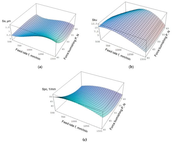
Figure 10.
Plot of the regression functions of roughness parameters: (a) Sa, (b) Sku, (c) Spc.
- for Sa (7):
- for Sku (8):
- for Spc (9):
Table 9 presents the R2 value and significance analysis (p-value) for individual structural elements of regression models for , and parameters. The R2 value shows the high accuracy of the models. As in the previous analyzes, the results indicate that not all structural elements of the model are statistically significant. However, attempts to omit them in the model resulted in a decrease in the quality of the model—a decrease in the value of R2.
Table 9.
R2 value and p-value for individual structural elements of regression models.
3.3. Microhardness
Plastic deformation of the weld made by the FSW method under the influence of the burnishing tool can be considered a process of generating new dislocations and moving them in the crystallites. At obstacles (grain boundaries, inclusions, slip bands), dislocations stop or bend, forming loops or half-loops lying in one crystallographic plane. As a result, the surface layer of the weld is strengthened, which is manifested by the formation of compressive stresses in the surface layer and an increase in its microhardness. The analysis of Figure 11 shows that regardless of the assumed feed rate, the microhardness of the surface layer increases with the increase in the tool burnishing force, reaching the maximum value at . For the feed rate , this corresponds to an increase in microhardness by 7.98% (to the value of ), for the feed rate of 24.01% (to the value of ) and for the feed rate of 9.11% (to the value of ). The reason for the decrease in the microhardness value may be a decrease in the value of the maximum stress in the area under the burnishing tip due to the increase in the contact surface. The stress distribution under the burnishing tip is uneven, and with some combination of burnishing force and contact area, it may happen that the stress is lower. This is particularly visible in the case of stresses in the transverse direction σx for variants no. 7–9 (Figure 3). At lower stress values, fewer structure defects are generated, resulting in lower microhardness. Further increasing the burnishing forcemay lead to exceeding the criticaldeformation value. As a result, the continuity of the material may be lost, and the fatigue strength of the joint may decrease.
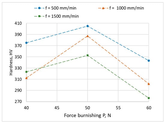
Figure 11.
Influence of feed rate and force burnishing on Vickers microhardness.
Based on the ANOVA analysis of variance, an adequate regression model of the surface layer hardness value (Figure 12) was developed at the significance level in the form (10):
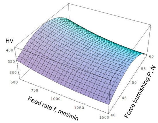
Figure 12.
Plot of the regression functions of microhardness.
Results of ANOVA analysis show that and are not statistically significant for HV (p-value 0.359 and 0.106). Table 10 presents the R2 value and significance analysis (p-value) for individual structural elements of regression models for HV. The R2 value shows the high accuracy of the models. The results indicate that not all structural elements of the model are statistically significant. However, attempts to omit them again in the model resulted in a decrease in the quality of the model—a decrease in the value of R2.
Table 10.
R2 value and p-value for individual structural elements of the regression model for HV.
3.4. Multi-Objective Optimization
Obtaining high reliability of joints made by the FSW method requires the selection of optimal parameters of the slide diamond burnishing. Proper selection of parameters should ensure the possibility of introducing high compressive stresses on the joint surface, hardening of the joint, and reduction of surface roughness to remove fatigue micro-notches that may reduce the fatigue strength of the joint. This selection must guarantee, apart from the required parameters of the surface layer, also high stability and efficiency of the process. This requires multi-criteria optimization and finding a compromise solution that meets the presented conditions.
The following notations were adopted for the presented multi-criteria problem:
- —a set of feasible solutions—the range of the SDB process parameters.
- x = (x1, x2, …, xm) —an acceptable solution.
- fi:E→R—i-th objective function (i = 1, 2,…, k).
- (x) = (f1(x), f2(x), …, f7(x)—objective function of a multi-criteria problem.
The problem of the multi-criteria optimization of the selection of the slide diamond burnishing process parameters can be written in the form (11):
In addition, the analysis took into account the process execution time t, which was determined as the quotient of the path traveled by the tool and the feed rate. For the feed rate of f = 500 mm/min, the specimen processing time was 2 min, while for the feed rate of f = 1500 mm/min 0.66 min.
A one-criteria problem written as (12) (in Table 11 was presented results):
is the i-th partial issue, while the vector in which the i-th objective functionachieves the extremum is the i-th partial solution. Vector (13)
is a vector called the ideal (utopian) solution in the evaluation space, whereas:
is the solution to the ideal problem.
φo = (f1(x1o), f2(x2o), …, f2(x7o))
xo = x1o, x2o, …, x7o
Table 11.
Results of one-criteria problem fi(x).
The set of efficient solutions usually contains many solutions. Therefore, the purpose of the presented problem was to select one solution from the set of effective solutions, called a compromise solution (compromise-optimal). For this purpose, issues (13) were reduced to a single-criterion form, with a scalarizing function in the form of (15):
The scalarization of the issue was carried out using the evaluation weighting method. The weight values individual criteria were adopted (meeting the condition ), and then the optimal solution of the problem was determined (16):
Creating the function is possible only when all objective functions are expressed in the same units and scales of values. Since, in the considered case, the objective functions were expressed in different scales of values, they were transformed into a dimensionless form taking values from the range [0, 1] for . After the unitarisation, an optimal solution to the problem is determined according to
The optimal solution of function (17) is an effective solution to the multi-criteria problem. The form of the solution depends on the adopted weight value . If it is assumed that all parameters have the same meaning (), the objective function achieves the minimum value for the feed rate and the burnishing force (Figure 13a). This makes it possible to obtain surface roughness parameters: µm, µm, and with the stress value in the surface layer and and microhardness . The parameters determined in this way also guarantee thehighest efficiency of the burnishing process (burnishing time ). If it is assumed for the calculations that the value of compressive stresses in the surface layer has the greatest impact on the fatigue strength of the joints (), a compromise solution can be obtained at the feed rate and the burnishing force (Figure 13b). Burnishing of joints with these parameters allows us to obtain the level of compressive stresses in the surface layer and . A higher value of compressive stresses is associated with the deterioration of the roughness parameters µm and with more rounded surface tops (), slightly higher microhardness of the surface layer of the joint () and significantly increased the time consuming of the burnishing process ().
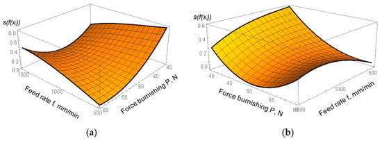
Figure 13.
Plot of the objective function of a multi-criteria optimization (a) ui = 0.142, (b) u1,2 = 0.25, u3–7= 0.1.
4. Conclusions
Research of the slide diamond burnishing process of butt joints made using the FSW method at a variable feed rate in the range of to and burnishing force in the range of to , carried out in accordance with the methodology of the PS/DC 32 plan, showed that:
- During friction stir welding, small tensile stresses (2 MPa) and grooves with an average depth of 9.77 μm (max 31.5 μm) are generated in the surface layer of the weld, which may contribute to a reduction in the fatigue strength of the joints.
- Burnishing enables the introduction of compressive stresses both in the transverse and longitudinal directions. Compressive stresses during exploitation add up to stresses from external forces, changing the symmetrical cycle into an asymmetric one with reduced, harmful tensile stresses, increasing the fatigue strength of the joints. The highest compressive stress value in the transverse direction was obtained with a burnishing force of and a feed rate of ), while in the longitudinal direction with a force of and a feed rate of ().
- Plastic deformation of the surface layer as a result of the burnishing process increases the microhardness of the surface layer of the weld from 84.19–174.53% and reduces the surface roughness Sa from 73.68–94.84%. This ensures a microgeometry of the surface characterized by large radii of the recesses and small angles of inclination of the sides of the irregularities, thus, eliminating geometric micro-cuts.
- Multi-criteria optimization of the burnishing process allows us to obtain a compromise solution ensuring compressive stresses in the surface layer ( and ) and microhardness with the roughness of the weld surface Sa = 0.28 µm, Sku = 3.93 and Spc = 35.88 1/mm, while ensuring high efficiency of the burnishing process.
- The highest microhardness was obtained at the force . By further increasing the burnishing force in the area under the diamond burnishing tip, the contact area increases, which in turn results in a decrease in the value of the maximum stress (especially in the transverse direction ). In the presence of lower stresses, fewer structural defects are created, which results in a decrease in the hardness of the surface layer of the joint.
Author Contributions
Conceptualization, M.B. and R.K.; methodology, M.B., R.K., K.A., A.D., W.B. and K.O.; software, M.B. and R.K.; validation, K.A., M.B. and R.K.; formal analysis, M.B., R.K., and A.D.; investigation, M.B., R.K., A.D, W.B. and K.O.; resources, M.B. and R.K.; data curation, R.K., A.D. and M.B.; writing—original draft preparation, M.B. and R.K. writing—review and editing, and M.B. and K.A.; visualization, R.K.; supervision, R.K. and M.B.; project administration, R.K. and M.B.; funding acquisition, K.A. All authors have read and agreed to the published version of the manuscript.
Funding
This research received no external funding.
Institutional Review Board Statement
Not applicable.
Informed Consent Statement
Not applicable.
Data Availability Statement
Not applicable.
Conflicts of Interest
The authors declare no conflict of interest.
References
- Lohwasser, D.; Chen, Z. Friction Stir Welding: From Basics to Applications; Elsevier: Amsterdam, The Netherlands, 2009. [Google Scholar]
- Kubit, A.; Trzepieciński, T.; Kluz, R.; Ochałek, K.; Slota, J. Multi-Criteria Optimisation of Friction Stir Welding Parameters for EN AW-2024-T3 Aluminium Alloy Joints. Materials 2022, 15, 5428. [Google Scholar] [CrossRef]
- Kashaev, N.; Ventzke, V.; Çam, G. Prospects of laser beam welding and friction stir welding processes for aluminum airframe structural applications. J. Manuf. Process. 2018, 36, 571–600. [Google Scholar] [CrossRef]
- Boldsaikhan, E.; Fukada, S.; Fujimoto, M.; Kamimuki, K.; Okada, H. Refill friction stir spot welding of surface-treated aerospace aluminum alloys with faying-surface sealant. J. Manuf. Process. 2019, 42, 113–120. [Google Scholar] [CrossRef]
- Vaneghi, A.H.; Bagheri, B.; Shamsipur, A.; Mirsalehi, S.E.; Abdollahzadeh, A. Investigations into the formation of intermetallic compounds during pinless friction stir spot welding of AA2024-Zn-pure copper dissimilar joints. Weld World. 2022, 66, 2351–2369. [Google Scholar] [CrossRef]
- He, Z.; Luo, Q.; Li, Q.; Zheng, G.; Sun, G. Fatigue behavior of CFRP/Al adhesive joints—Failure mechanisms study using digital image correlation (DIC) technique. Thin-Walled Struct. 2022, 174, 109075. [Google Scholar] [CrossRef]
- Su, J.Q.; Nelson, T.W.; Mishra, R.; Mahoney, M. Microstructural investigation of friction stir welded 7050-T651 aluminum. Acta Mater. 2003, 51, 713–729. [Google Scholar] [CrossRef]
- Hatamleh, O.; DeWald, A. An investigation of the peening effects on the residual stresses in friction stir welded 2195 and 7075 aluminum alloy joints. J. Mater. Process. Technol. 2009, 209, 4822–4829. [Google Scholar] [CrossRef]
- Shrivastava, A.; Krones, M.; Pfefferkorn, F.E. Comparison of energy consumption and environmental impact of friction stir welding and gas metal arc welding for aluminum. CIRP J. Manuf. Sci. Technol. 2015, 9, 159–168. [Google Scholar] [CrossRef]
- Cabibbo, M.; Meccia, E.; Evangelista, E. TEM analysis of a friction stir-welded butt joint of Al–Si–Mg alloys. Mater. Chem. Phys. 2003, 81, 289–292. [Google Scholar] [CrossRef]
- Krasnowski, K.; Hamilton, C.; Dymek, S. Influence of the tool shape and weld configuration on microstructure and mechanical properties of the Al 6082 alloy FSW joints. Arch. Civ. Mech. Eng. 2015, 15, 133–141. [Google Scholar] [CrossRef]
- Zielecki, W.; Bucior, M.; Trzepiecinski, T.; Ochał, K. Effect of slide burnishing of shoulder fillets on the fatigue strength of X19NiCrMo4 steel shafts. J. Adv. Manuf. Technol. 2020, 106, 2583–2593. [Google Scholar] [CrossRef]
- Teimouri, R.; Grabowski, M.; Bogucki, R.; Ślusarczyk, Ł.; Skoczypiec, S. Modeling of strengthening mechanisms of surface layers in burnishing process. Mater. Des. 2022, 223, 111114. [Google Scholar] [CrossRef]
- Korzyński, M.; Pacana, A.; Cwanek, J. Fatigue strength of chromium coated elements and possibility of its improvement with slide diamond burnishing. Surf. Coat. Technol. 2009, 203, 1670–1676. [Google Scholar] [CrossRef]
- Han, K.; Tan, L.; Yao, C.; Zhang, D.; Zhou, Z. Studies on the surface characteristics of Ti60 alloy induced by turning combined with ball burnishing. J. Manuf. Process. 2022, 76, 349–364. [Google Scholar] [CrossRef]
- Silva-Álvarez, D.F.; Márquez-Herrera, A.; Saldaña-Robles, A.; Zapata-Torres, M.; Mis-Fernández, R.; Peña-Chapa, J.L.; Moreno-Palmerín, J.; Hernández-Rodríguez, E. Improving the surface integrity of the CoCrMo alloy by the ball burnishing technique. J. Mater. Res. Technol. 2020, 9, 7592–7601. [Google Scholar] [CrossRef]
- Barahate, V.; Govande, A.R.; Tiwari, G.; Sunil, B.R.; Dumpala, R. Parameter optimization during single roller burnishing of AA6061-T6 alloy by design of experiments. Mater. Today Proc. 2022, 50, 1967–1970. [Google Scholar] [CrossRef]
- Kubit, A.; Bucior, M.; Kluz, R.; Święch, Ł.; Ochał, K. Application of the 3d digital image correlation tothe analysis of deformation of joints welded withthe FSW method after shot peening. Adv. Mater. Sci. Eng. 2019, 19, 57–66. [Google Scholar] [CrossRef]
- Korzyński, M. Slide Burnishing; WNT: Warsaw, Poland, 2009. [Google Scholar]
- Raza, A.; Kumar, S. A critical review of tool design in burnishing process. Tribol. Int. 2022, 174, 107717. [Google Scholar] [CrossRef]
- Konefal, K.; Korzynski, M.; Byczkowska, Z.; Korzynska, K. Improved corrosion resistance of stainless steel X6CrNiMoTi17-12-2 by slide diamond burnishing. J. Mater. Process. Technol. 2013, 213, 1997–2004. [Google Scholar] [CrossRef]
- Duncheva, G.V.; Maximov, J.T.; Anchev, A.P.; Dunchev, V.P.; Argirov, Y.B.; Kandeva-Ivanova, M. Enhancement of the wear resistance of CuAl9Fe4 sliding bearing bushings via diamond burnishing. Wear 2022, 510–511, 204491. [Google Scholar] [CrossRef]
- Dzierwa, A.; Gałda, L.; Tupaj, M.; Dudek, K. Investigation of wear resistance of selected materials after slide burnishing process. Eksploat. Niezawodn. Maint. Reliab. 2020, 22, 432–439. [Google Scholar] [CrossRef]
- Nestler, A.; Schubert, A. Effect of Machining Parameters on Surface Properties in Slide Diamond Burnishing of Aluminium Matrix Composites. Mater. Today Proc. 2015, 2, S156–S161. [Google Scholar] [CrossRef]
- Rodríguez, A.; Calleja, A.; López de Lacalle, L.N.; Pereira, O.; González, H.; Urbikain, G.; Laye, J. Burnishing of FSW Aluminum Al–Cu–Li Components. Metals 2019, 9, 260. [Google Scholar] [CrossRef]
- Sánchez Egea, A.J.; Rodríguez, A.; Celentano, D.; Calleja, A.; López de Lacalle, L.N. Joining metrics enhancement when combining FSW and ball-burnishing in a 2050 aluminium alloy. Surf. Coat. Technol. 2019, 367, 327–335. [Google Scholar] [CrossRef]
- Pontes, F.J.; Amorim, G.F.; Balestrassi, P.P.; Paiva, A.P.; Ferreira, J.R. Design of experiments and focused gridsearch for neural network parameter optimization. Neurocomputing 2016, 186, 22–34. [Google Scholar] [CrossRef]
- Kluz, R.; Antosz, K.; Trzepiecinski, T.; Bucior, M. Modelling the influence of slide burnishing parameters on the surface roughness of shafts made of 42CrMo4 heat-treatable steel. Materials 2021, 14, 1175. [Google Scholar] [CrossRef]
- Merisalu, M.; Aarik, L.; Kozlova, J.; Mändar, H.; Tarre, A.; Sammelselg, V. Effective corrosion protection of aluminum alloy AA2024-T3 with novel thin nanostructured oxide coating. Surf. Coat. Technol. 2021, 411, 126993. [Google Scholar] [CrossRef]
- Kaushik, Y.; Jawalkar, C.S.; Kan, S. A review on use of aluminium alloys in aircraft components. I-Manager’s J. Mater. Sci. 2015, 3, 33–38. [Google Scholar]
- ASTMB209M; Standard Specification for Aluminum and Aluminum-Alloy Sheet and Plate. ASTM International: West Conshohocken, PA, USA, 2014.
- Bonarski, J.T. Measurement and Use of the Texture-Stress Microstructure Characteristics in Materials Diagnostics; Institute of Metallurgy and Materials Science of the Polish Academy of Sciences: Cracow, Poland, 2013. (In Polish) [Google Scholar]
- ISO 25178-2:2012; Geometrical Product Specifications (GPS); Surface Texture: Areal—Part 2: Terms, Definitions and Surface Texture Parameters. International Organization for Standarization: Geneva, Switzerland, 2012.
- Abbasi, M.; Abdollahzadeh, A.; Bagheri, B.; Ostovari Moghaddam, A.; Sharifi, F.; Dadaei, M. Study on the effect of the welding environment on the dynamic recrystallization phenomenon and residual stresses during the friction stir welding process of aluminum alloy. Proc. Inst. Mech. Eng. L J. Mater. Des. Appl. 2021, 235, 1809–1826. [Google Scholar] [CrossRef]
- Bagheri, B.; Abbasi, M.; Hamzeloo, R. The investigation into vibration effect on microstructure and mechanical characteristics of friction stir spot vibration welded aluminum: Simulation and experiment. Proc. Inst. Mech. Eng. Part C J. Mech. Eng. Sci. 2020, 234, 1809–1822. [Google Scholar] [CrossRef]


Disclaimer/Publisher’s Note: The statements, opinions and data contained in all publications are solely those of the individual author(s) and contributor(s) and not of MDPI and/or the editor(s). MDPI and/or the editor(s) disclaim responsibility for any injury to people or property resulting from any ideas, methods, instructions or products referred to in the content. |
© 2023 by the authors. Licensee MDPI, Basel, Switzerland. This article is an open access article distributed under the terms and conditions of the Creative Commons Attribution (CC BY) license (https://creativecommons.org/licenses/by/4.0/).