Neural Network-Based Approach to Detect and Filter Misleading Audio Segments in Classroom Automatic Transcription

Abstract

Audio recording in classrooms is a common practice in educational research, with applications ranging from detecting classroom activities to analyzing student behavior. Previous research has employed neural networks for classroom activity detection and speaker role identification. However, these recordings are often affected by background noise that can hinder further analysis, and the literature has only sought to identify noise with general filters and not specifically designed for classrooms. Although the use of high-end microphones and environmental monitoring can mitigate this problem, these solutions can be costly and potentially disruptive to the natural classroom environment. In this context, we propose the development of a novel neural network model that specifically detects and filters out problematic audio sections in classroom recordings. This model is particularly effective in reducing transcription errors, achieving up to a 96% success rate in filtering out segments that could lead to incorrect automated transcriptions. The novelty of our work lies in its targeted approach for low-budget, aurally complex environments like classrooms, where multiple speakers are present. By allowing the use of lower-quality recordings without compromising analysis capability, our model facilitates data collection in natural educational settings and reduces the dependency on expensive recording equipment. This advancement not only demonstrates the practical application of specialized neural network filters in challenging acoustic environments but also opens new avenues for enhancing audio analysis in educational research and beyond.

1. Introduction

Noise in audio recordings is a persistent problem that can significantly hinder the analysis and interpretation of collected data. This issue is particularly pronounced in noisy environments like classrooms, where a variety of noise sources can interfere with the recording quality [1]. These noises can come from a variety of sources, including background student chatter, classroom ambient noise, and heating and cooling system noise. The unpredictable nature of these noise sources makes their removal from recordings a challenge [2].

To address these challenges, we have implemented the use of a lavalier microphone carried by the teacher, specifically designed to capture the teacher’s speech. This microphone transmits via a UHF signal to a cell phone placed at the back of the classroom. Employing this method ensures the teacher’s talk is predominantly recorded, mitigating privacy concerns as the cell phone mic could inadvertently record both audio and video of students. Furthermore, this setup synchronizes all recordings on a single device. This contrasts with previous studies that recorded video and audio separately and then had to synchronize them, a non-trivial task due to inadvertent interruptions. We use the UHF signal to avoid consuming wifi bandwidth, which is scarce in classrooms. However, the signal can occasionally be interrupted when the teacher moves around the classroom, and it can also occasionally introduce noise. In addition to this, the teacher could carry the necessary equipment (cell phone, microphone, and small tripod, as detailed in Section 3) in a carry-on bag and could take them to other classrooms and even to other schools. This practical and inexpensive solution was key to achieving the scale of recordings we were able to obtain.

Classrooms are inherently complex and noisy environments due to the nature of the activities carried out in them. Students may be talking amongst themselves, teachers may be giving instructions, and there may be background noise from class materials and other equipment. The presence of multiple speakers and poor acoustics further complicates the process of noise reduction and speaker identification [1].

Collaborative learning environments can be particularly challenging when it comes to speaker identification in noisy audio recordings [2]. In these contexts, the task of identifying individual students speaking in small clusters amidst other simultaneous conversations becomes exceptionally complex. This difficulty underscores the demand for efficient strategies in detecting and filtering noise in classroom recordings. Despite these challenges, the development of advanced techniques such as deep learning and neural networks has shown promise in improving noise detection and filtering in classroom recordings [3,4,5].

A significant issue in classrooms arises when background noises are too similar to the teacher’s voice, making it challenging for a simple audio enhancement to filter out the noise from the voice. When attempting to use a state-of-the-art automatic transcriber like Whisper [6], we encountered not only regular transcription issues but also hallucinations that generated entirely fabricated sentences unrelated to the context of the recording (Figure 1).

In other instances, phrases like “Voy a estar en la iglesia!” (“I’ll be at the church!”) or “Se pide al del cielo y le ayuda a la luz de la luz”. (“He asks the one from the sky and he helps with the light of the light”.) appeared out of nowhere (in non-talking segments) in a mathematics class, contaminating any analysis of the content of those audio segments.

Our study demonstrates that the proposed filter significantly improves the quality of transcriptions, especially in environments with a high proportion of poor-quality segments. This approach not only aids in creating better datasets for speech enhancement models but also substantially reduces transcription errors and hallucinations, as exemplified in our analysis of different teaching sessions. Thus, our work addresses a critical need for accurate and efficient transcription in educational settings, where traditional methods may fall short due to the complex nature of classroom noise.

While some studies have explored multimodal methods for speaker identification using both visual and acoustic features [7], the focus of this work is solely on acoustic features. The goal is to leverage the power of neural networks to detect and filter the best-quality audio segments from classroom recordings, without the need for visual cues or enhancements to the audio during recording.

Moreover, while speech enhancement and inverse filtering methods have shown promise in improving speech intelligibility in noisy and reverberant environments [8], the aim of this work is not to improve the audio during recording. Instead, the focus is on post-recording, using a simple, low-cost recording setup such as a teacher’s mobile phone. The proposed algorithm does not enhance the audio but selects the best-quality audio segments for transcription. This approach not only facilitates the creation of high-quality datasets for speech enhancement models but also improves the transcriptions. By avoiding the transcription of intervals with higher noise levels, it reduces hallucinations and achieves improvements that cannot be obtained by merely adjusting the parameters of transcription tools like Whisper.

Finally, this work employs a specific classifier to select high-quality segments for transcription. This approach has the potential to improve the results of transcription systems like Whisper, which are trained on a broad and diverse distribution of audio and evaluated in a zero-shot setting, thereby moving closer to human behavior [6].

In this context, the proposal of a neural network model that can specifically detect and filter background noises in classroom recordings presents a promising solution to this persistent problem. The development of these efficient strategies is crucial for improving the quality of data collected and facilitating its analysis and interpretation [2,3,5].

2. Related Work

Sound detection, and particularly the identification of noises from various sources, has as many applications as varied as the places where these noises can be found. In this section, we summarize several works found in the literature that pertain to the diverse applications, approaches, and systems devised for this task across a multitude of contexts. This will provide perspective on the contribution and positioning of our work in relation to the studies showcased in this section.

Of notable mention is the work by Sabri et al. [9], who in 2003 developed an audio noise detection system using the hidden Markov model (HMM). They aimed to classify aircraft noise with an $83\%$ accuracy, using 15 training signals and 28 testing signals. The system combined linear prediction coefficients with cepstrum coefficients and employed vector quantization based on fuzzy C-mean clustering. This pioneering work, developed before the significant expansion of neural networks in noise detection, has influenced many environments and could even extend to settings such as classrooms.

Another significant work around noise detection was developed by Rangachari and Loizou [10], who proposed a noise-estimation algorithm for highly non-stationary environments, such as a classroom or a busy street, where noise characteristics change rapidly. The algorithm updates the noise estimate using a time-frequency dependent smoothing factor, computed based on the speech-presence probability. This method adapts quickly to changes in the noise environment, making it suitable for real-time applications. The algorithm was found to be effective when integrated into speech enhancement, outperforming other noise-estimation algorithms, and has potential applications in improving the quality of speech communication in noisy settings.

In the domain of voice activity detection (VAD), the influential study by Zhang and Wu [4] stands out for its pioneering approach to addressing the challenges of real-world noisy data. Their research introduces a methodology based on denoising deep neural networks (DDNNs) for VAD, capitalizing on the network’s ability to learn robust features amidst noise. Unlike many traditional systems that lean on clean datasets, this method emphasizes unsupervised denoising pre-training, followed by supervised fine-tuning. This design ensures the model adeptly adapts to real-world noisy data. Once the network undergoes pre-training, it is fine-tuned to mimic the characteristics of clean voice signals. The essence of this approach is its adaptability and proficiency in real-world scenarios, showcasing significant enhancement in voice activity detection amidst noise.

In the realm of polyphonic sound event detection, the work by Çakır et al. [11] stands out for its innovative approach using multi-label deep neural networks (DNNs). The study was aimed at detecting multiple sound events simultaneously in various everyday contexts, such as basketball matches and busy streets, where noise characteristics are complex and varied. The proposed system, trained on 103 recordings from 10 different contexts, totaling 1133 min, employed DNNs with 2 hidden layers and log Mel-band energy features. It outperformed the baseline method by a significant margin, offering an average increase in accuracy of $19\%$. The adaptability and effectiveness of this method in handling polyphonic sound detection make it a valuable contribution to the field of noise detection. It emphasizes the potential of DNNs in accurately identifying noises from various sources and sets a precedent for future research in enhancing real-time audio communication in noisy environments.

The paper by Dinkel et al. [12] proposes a cutting-edge method that overcomes the difficulties of actual noisy data in the rapidly changing environment of Voice Activity Detection (VAD). Their study provides a teacher-student model for VAD that is data-driven and uses vast, unrestricted audio data for training. This approach only requires weak labels, which are a form of supervision where only coarse-grained or ambiguous information about the data are available (e.g., a label for an entire audio clip rather than precise frame-by-frame annotations) during the teacher training phase. In contrast, many conventional systems rely extensively on clean or artificially noised datasets. A student model on an unlabeled target dataset is given frame-level advice by the teacher model after it has been trained on a source dataset. This method’s importance rests in its capacity to extrapolate to real-world situations, showing significant performance increases in both artificially noisy and real-world settings. This study sets a new standard for future studies in this field by highlighting the potential of data-driven techniques in improving VAD systems, particularly in settings with unexpected and diverse noise characteristics.

An interesting approach can be found in the work of Rashmi et al. [13], where the focus is on removing noise from speech signals for Speech-to-Text conversion. Utilizing PRAAT, a phonetic tool, the study introduces a training-based noise-removal technique (TBNRT). The method involves creating a noise class by collecting around 500 different types of environmental noises and manually storing them in a database as a noise tag set. This tag set serves as the training data set, and when input audio is given for denoising, the corresponding type of noise is matched from the tag set and removed from the input data without tampering with the original speech signal. The study emphasizes the challenges of handling hybrid noise and the dependency on the size of the noise class. The proposed TBNRT has been tested with various noise types and has shown promising results in removing noise robustly, although it has limitations in identifying noise containing background music. The approach opens up possibilities for future enhancements, including applications in noise removal stages in End Point Detection of continuous speech signals and the development of speech synthesis with emotion identifiers.

A significant contribution to this field is the work by Kartik and Jeyakumar [14], who developed a deep learning system to predict noise disturbances within audio files. The system was trained on $1,282,239$ training files, and during prediction, it generates a series of 0 s and 1 s in intervals of 10 ms, denoting the ‘Audio’ or ‘Disturbance’ classes (Total of 3 h and 33 min). The model employs dense neural network layers for binary classification and is trained with a batch size of 32. The performance metrics, including training accuracy of $90.50\%$ and validation accuracy of $83.29\%$, demonstrate its effectiveness. Such a system has substantial implications in preserving confidential audio files and enhancing real-time audio communication by eliminating disturbances.

In the realm of speech enhancement and noise reduction, the work of Yan Zhao et al. [15] in “DNN-Based Enhancement of Noisy and Reverberant Speech” offers a significant contribution. Their study introduces a deep neural network (DNN) approach to enhance speech intelligibility in noisy and reverberant environments, particularly for hearing-impaired listeners. The algorithm focuses on learning spectral mapping to enhance corrupted speech by targeting reverberant speech, rather than anechoic speech. This method showed promising results in improving speech intelligibility under certain conditions, as indicated by preliminary listening tests. The DNN architecture employed in their study includes four hidden layers with 1024 units each, using a rectified linear function (ReLU) for the hidden layers and sigmoidal activation for the output layer. The algorithm was trained using a mean square error loss function and employed adaptive gradient descent for optimization. Objective evaluation of the system using standard metrics like short-time objective intelligibility (STOI) and the perceptual evaluation of speech quality (PESQ) demonstrated significant improvements in speech intelligibility and quality. This work aligns well with the broader objectives of enhancing audio quality in challenging acoustic environments with a specific focus on aiding hearing-impaired listeners.

In a similar vein to the previously discussed works, the study conducted by Ondrej Novotny et al. [16] presents a noteworthy advance in the field of speech processing. This paper delves into the application of a deep neural network-based autoencoder for enhancing speech signals, particularly focusing on robust speaker recognition. The study’s key contribution is its approach to using the autoencoder as a preprocessing step in a text-independent speaker verification system. The model is trained to learn a mapping from noisy and reverberated speech to clean speech, using the Fisher English database for training. A significant finding of this study is that the enhanced speech signals can notably improve the performance of both i-vector and x-vector based speaker verification systems. Experimental results show a considerable improvement in speaker verification performance under various conditions, including noisy and reverberated environments. This work underscores the potential of DNN-based signal enhancement in enhancing the accuracy and robustness of speaker verification systems, which complements the objectives of this study that focus on improving classroom audio transcription through neural networks.

In a noteworthy parallel to the realm of audio signal processing for educational purposes, the research conducted by Coro et al. [17] explores the domain of healthcare simulation training. Their innovative approach employs syllabic-scale speech processing and unsupervised machine learning to automatically highlight segments of potentially ineffective communication in neonatal simulation sessions. The study, conducted on audio recordings from 10 simulation sessions under varied noise conditions, achieved a detection accuracy of 64% for ineffective communication. This methodology significantly aids trainers by rapidly pinpointing dialogue segments for analysis, characterized by emotions such as anger, stress, or misunderstanding. The workflow’s ability to process a 10-min recording in approximately 10 s and its resilience to varied noise levels underline its efficiency and robustness. This research complements the broader field of audio analysis in challenging environments by offering an effective model for evaluating human factors in communication, which could be insightful for similar applications in educational settings, paralleling the objectives of enhancing audio transcription accuracy in classroom environments.

While the research studies cited above have achieved substantial advances in noise detection and classification, there is still a large gap in tackling the unique issues provided by primary school classroom situations. These environments have distinct noise profiles that are frequently modified by student interactions, classroom activities, and the natural acoustics of the space. Unlike previous work, our research also focuses on the classification aimed at predicting the quality of audio-to-text transcriptions in the classroom environment. Furthermore, the feasibility of applying these methods in real-world applications has not been thoroughly investigated, particularly given budget limits that necessitate the use of low-cost UHF microphones and the requirement for distant detection (e.g., a smartphone put at a distance). Our research aims to close this gap by concentrating on the intricacies of noise interference in primary schools, particularly when employing low-cost equipment.

Given this context, our research questions are:

• “To what extent can we enhance information acquisition from transcriptions in elementary school classes by eliminating interferences and noises inherent to such settings, using an affordable UHF microphone transmitting to a smartphone located 8 m away at the back of the classroom?”
• “To what extent can we ensure that, in our pursuit to enhance transcription quality by eliminating noises and interferences, valuable and accurate information is not inadvertently filtered out or omitted in the process?”

3. Materials and Methods

3.1. Materials and Costs Associated with Data Collection

Video and audio recordings were carried out by trained teachers using low-cost equipment. The devices used for video recordings were Redmi 9A (Manufacturer: Xiaomi, Origin: China/India, purchased from Aliexpress) mobile phones with 2 GB of RAM and 32 GB of ROM. For audio recordings, lavalier UHF (Brand: Ulanzi, Origin: CN(China), purchased from Aliexpress) lapel microphones were used. In addition, small tripods were used to hold the mobile phones during the recordings.

The costs of the equipment used are detailed in

Table 1. Costs of the equipment used for video and audio recordings.

Equipment	Cost (Chilean Pesos)	Cost (USD)
Redmi 9A Mobile Phone	70,000	90
Lavalier UHF Lapel Microphone	17,000	20
Mobile Phone Tripod	5000	6
Total per teacher	92,000	116

.

For a proper understanding of the cost, consider that each teacher taught around 20 h of classes weekly. In a typical year, classes are held for 30 weeks, which amounts to 600 h annually. Considering that the costs in the table are fixed for a specific year, we can estimate the cost per class hour for the materials as follows:

$${\displaystyle \frac{\mathrm{Annual}\mathrm{investment}}{\mathrm{Annual}\mathrm{class}\mathrm{hours}}}={\displaystyle \frac{116}{600}}\approx 0.1933(\mathrm{USD}\mathrm{per}\mathrm{hour})$$

Given an average of 29 students per class, the cost per student is:

$${\displaystyle \frac{0.1933}{29}}\approx 0.0067(\mathrm{USD}\mathrm{per}\mathrm{student}\mathrm{per}\mathrm{hour})$$

In total, 14 mobile phones were used for the recordings, representing a total investment of approximately USD 1624.

3.2. Data Collection

From May to December, we recorded a total of 2079 educational videos and then subjected them to preprocessing and quality control. This step was necessary because many videos had audio issues, primarily due to defective microphones. After the quality control process, 1424 out of the 2079 original videos met our standards for audio problem detection. We then selected a representative sample of 14 videos from these, featuring a variety of instructors with distinct voices. From these 14 videos, we randomly chose and labeled 945 segments, each 10 s long, for further analysis. This section will detail the entire process, from the initial recording to the final segment selection.

3.3. Preprocessing and Quality Control

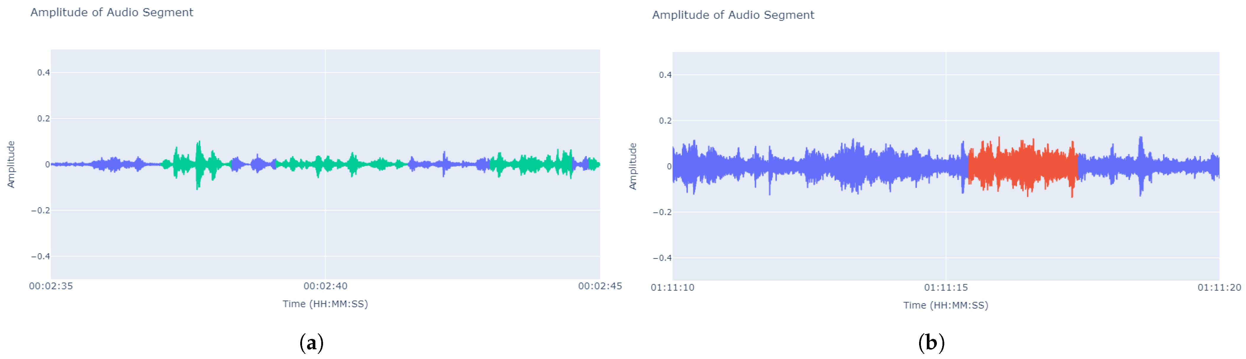
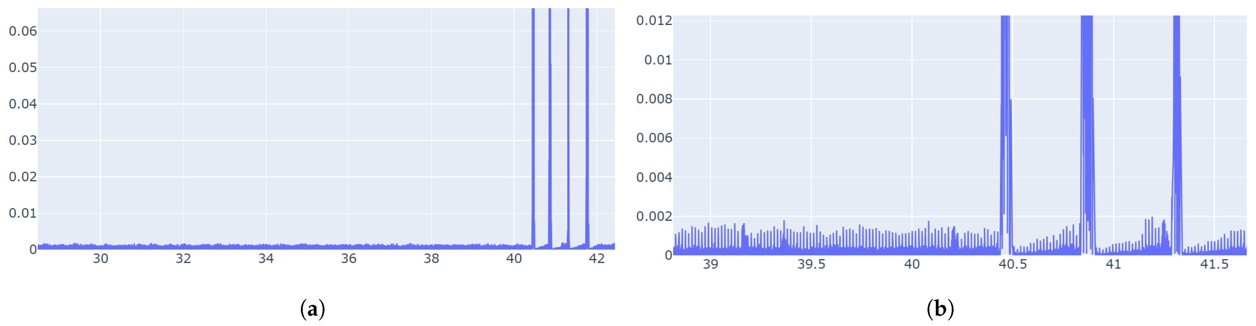
We obtained the 2079 recordings and then conducted a quality diagnosis to filter out low-quality recordings. The filtering algorithm took uniformly distributed samples from the audio of each class’s recordings. For each sample, we calculated the 50th percentile of the volume (or amplitude) of all the frames in the audio segment. If this percentile fell below an established empirical value (less than 0.005), a level that can be deduced from Figure 2 and Figure 3 and is lower than common background noise, we considered that sample to have audio quality problems. If over $30\%$ of the samples from a specific class recording had audio issues, we deemed the entire recording as low quality and discarded it.

3.4. Data Labeling and Augmentation

We filtered the recordings and then embarked on the task of labeling randomly selected 10-second segments as “acceptable” or “not acceptable” for transcription. This process resulted in a total of 945 labeled segments, amounting to approximately 158 min. The labeling criteria included categories such as “Unintelligible Content”, “Nothing to Transcribe”, “Indistinguishable Noise”, “Understandable but Low Volume”, “Understandable with Noise”, and “Clear and Noise-free”. These criteria were then grouped into quality categories “Ideal”, “Good”, “Fair”, and “Poor”, which were ultimately simplified to “Acceptable” or “Not Acceptable”. This categorization was implemented to enhance interpretability for future modeling efforts.

To summarize the labeling, if the professor’s speech was acceptably clean and understandable, the segment received an “acceptable” label. If the segment included external noises like white noise, dialogues from children, shouts, or chair movements, or if understanding the professor was difficult, the segment received a “not acceptable” label.

Recognizing the need to increase the quantity of data and mitigate any bias where volume might disproportionately influence noise detection, we implemented a data augmentation strategy. It is important to note that the clarity of an audio segment for transcription is not determined by its volume but rather by its content and interference. This is because the person labeling the audio segments had the flexibility to adjust the volume or use headphones as needed, making the volume of the segment non-determinative for labeling. However, there exists a range of volume levels within which automatic transcription tools can effectively operate.

To increase the quantity of data and mitigate biases related to volume levels, we implemented a data augmentation strategy. Our algorithm first measures the current volume of each segment in decibels full scale (dBFS). It then calculates the difference between this current volume and a set of predefined optimal volume levels, ranging from −20 dBFS to −28 dBFS (determined based on the volume analysis of the most intelligible audio segments). The algorithm selects the smallest difference, corresponding to the closest predefined volume level that is still greater than the current volume of the segment.

For example, if an original audio segment had a volume of −18 dBFS, the algorithm would lower it to −20 dBFS. Conversely, if a segment had a volume of −32 dBFS, the algorithm would raise it to −28 dBFS.

Moreover, to ensure that the volume of the augmented segment does not match the volume of the original segment, an element of randomness is introduced into the process. After adjusting the volume to the nearest optimal level, a random value is generated and added to the volume of the segment. This random value is either between −1.5 and −0.5 or between 0.5 and 1.5, ensuring a minimum alteration of 0.5 dBFS from the original adjusted volume level.

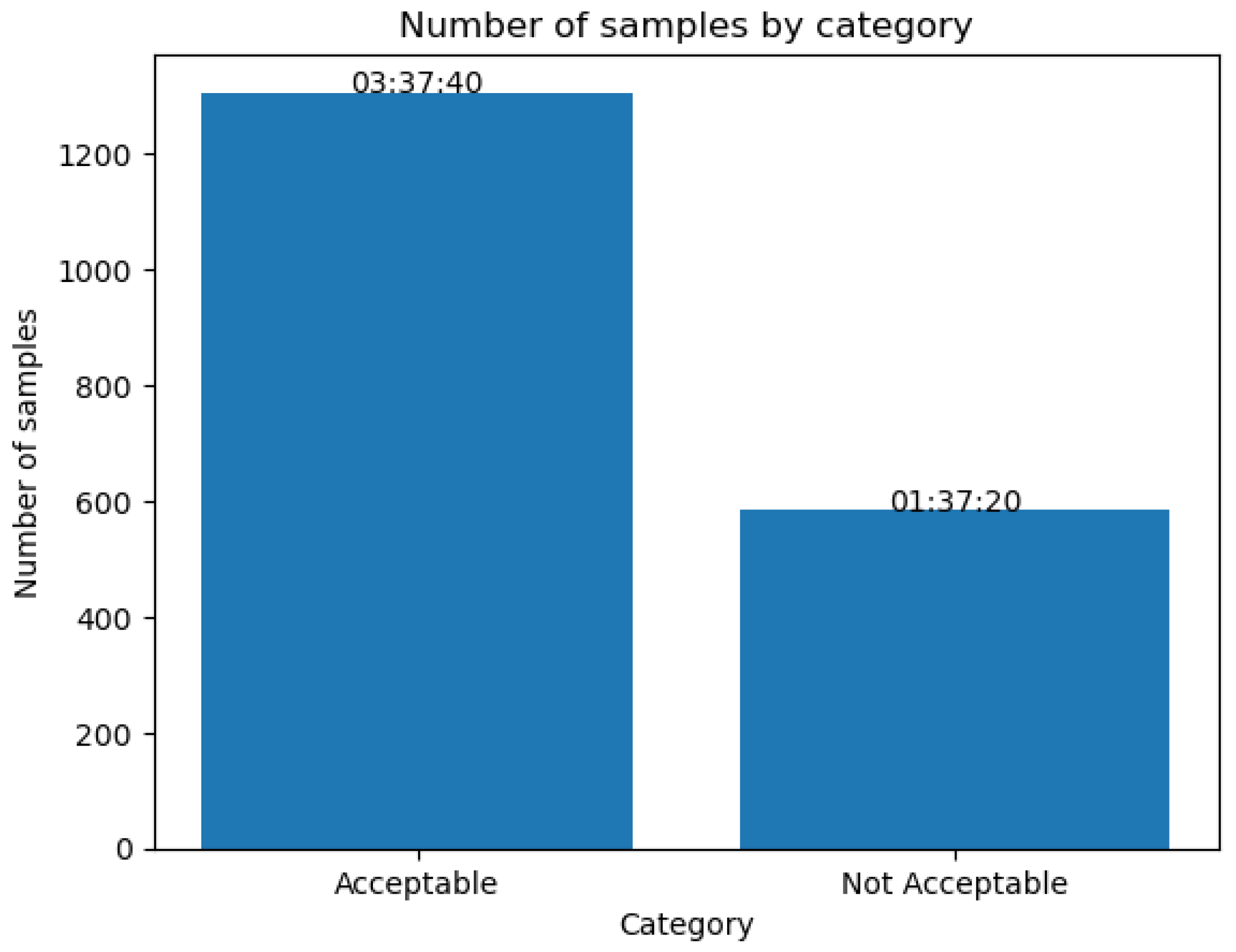
We then adjust the volume of each segment by this calculated difference. This effectively raises the volume of segments below the target range and lowers the volume of those above it. By applying this algorithm to each of the original 945 segments, we created an additional set of 945 segments with adjusted volumes. This doubled our dataset to a total of 1890 segments, each labeled as “Acceptable” or “Not Acceptable” depending on whether or not it was possible to recognize what was being said in the transcript. The sum of the two classes gave a total time of 5 h and 15 min, their distribution is detailed in Figure 4.

This approach not only made our dataset more robust but also ensured it was unbiased, setting the stage for more reliable subsequent analysis. Additionally, while the model was trained using the proportion of segments indicated in Figure 4, we explored the use of balancing techniques such as SMOTE [18] to ensure that the model is not biased towards the majority category. This exploration revealed that certain training metrics could be improved with balancing methods. The metrics with and without the application of such balancing techniques are detailed in the results section (Section 4.1.1), specifically in

Table 2. We take the metrics with respect to the “Not Acceptable” class from the randomly separated training set since the main purpose of the filter is to predict this class.

Data	Precision	Accuracy	Recall	F1	AUC
train	0.703	0.823	0.751	0.726	0.835
test	0.631	0.782	0.646	0.639	0.810

,

Table 3. Metrics with respect to the “Not Acceptable” class with balanced data.

Data	Precision	Accuracy	Recall	F1	AUC
train	0.821244	0.820767	0.826597	0.823912	0.903006
test	0.756757	0.780423	0.786517	0.771350	0.878048

and

Table 4. Metrics with respect to the “Acceptable” class with balanced data.

Data	Precision	Accuracy	Recall	F1	AUC
train	0.820270	0.820767	0.814765	0.817508	0.096994
test	0.803109	0.780423	0.775000	0.788804	0.121952

.

3.5. Audio Features

To train the neural network, we extracted a series of audio features associated with audio quality. These features include the deciles of the audio volume level, which divide the data into intervals containing equal proportions of the data. We also considered the average and standard deviation of these deciles, which measure the central tendency and dispersion of the audio volume level.

Frequencies play a crucial role in audio quality, so we included several frequency-related parameters. These parameters encompass the Mel-frequency cepstral coefficients (MFCCs), which capture the power spectrum of the audio signal; the spectral contrast, which measures the difference in amplitude between peaks and valleys in the sound spectrum; and the pitch, which orders sounds on a frequency-related scale based on their perceptual property.

We also incorporated parameters related to the shape of the power spectrum, such as the spectral centroid and bandwidth, which measure the “center of mass” and spread of the power spectrum, respectively; the spectral rolloff, which indicates the frequency below which a specified percentage of the total spectral energy resides; and the zero crossing rate, which tracks the rate that a signal changes from positive to zero to negative, or from negative to zero to positive.

From all these parameters, we discarded those with a correlation to the classification of interest that was too close to 0 (an absolute distance of less than 0.1). In the end, we selected only 26 from the original 38 input parameters for the final model.

The list of parameters and their correlations can be found in Appendix A.

3.6. Model Architecture and Training

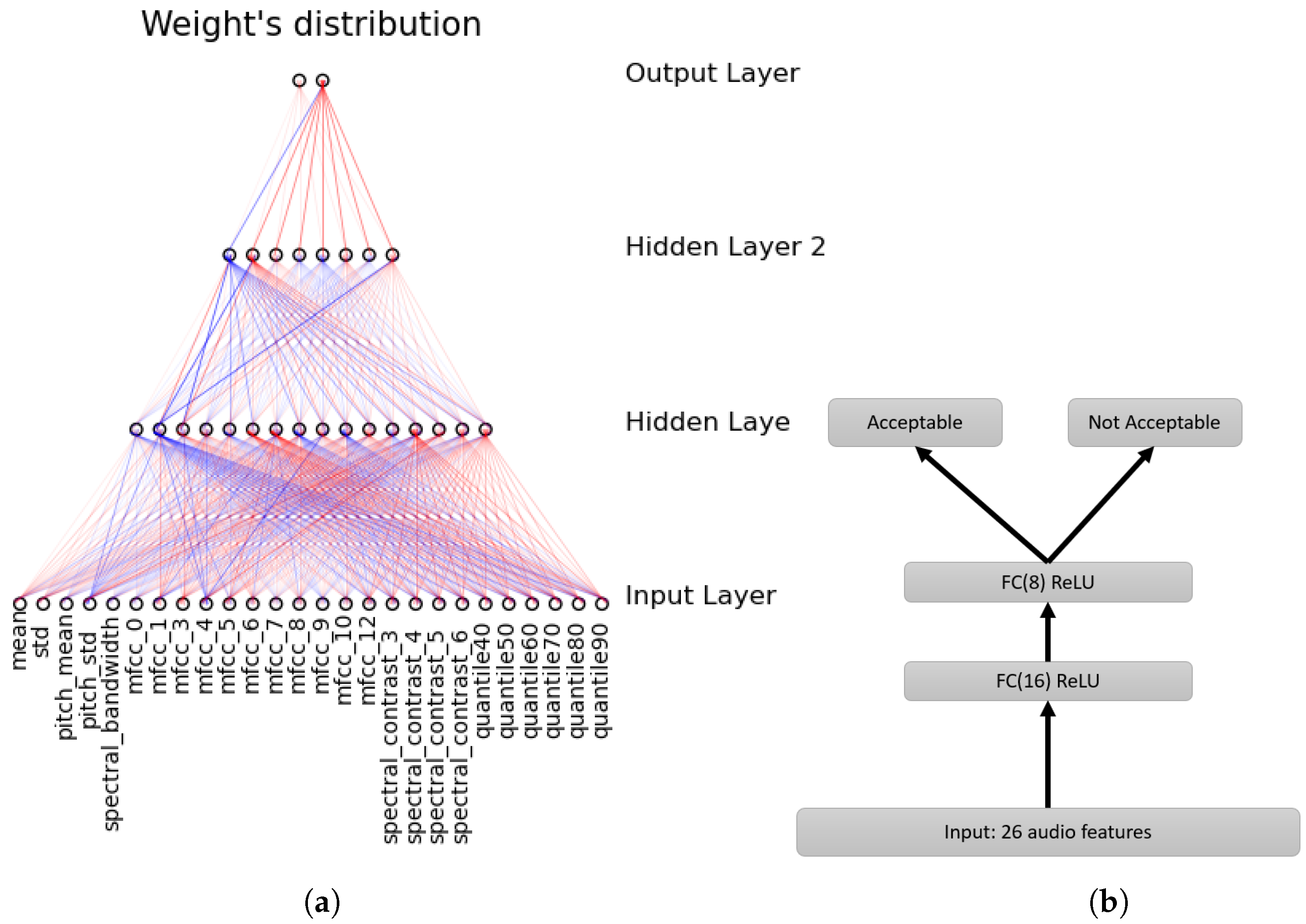
The proposed model is a classification network designed with the complexity of the task at hand in mind. It consists of two hidden layers with 16, and 8 neurons, respectively, summing up to a total of 24 neurons (without counting the input layer of 26 and the output of 2). The final layer has two neurons corresponding to the classification categories, reflecting the nature of the output parameters (Figure 5b).

While the choice of the number of hidden layers and the nodes within each is often a subject of debate, the architecture of a classification model is largely dictated by the inherent complexity of the patterns one seeks to discern within the dataset. In our context, the objective is for our neural network to make informed decisions based on the characteristics of an audio sample. This necessitates, at a minimum, the ability to understand patterns from the audio’s waveform plot. Two hidden layers have the capability to represent an arbitrary decision boundary with arbitrary accuracy using rational activation functions and can approximate any smooth mapping to any desired precision [19]. The decision to employ only 2 hidden layers was made after noting that adding more layers did not yield significant performance improvements during our tests. This observation aligns with findings reported for neural networks of a similar size in prior research, such as that by [20].

For the node count in each hidden layer, we adhered to the general “2/3” rule, suggesting that one layer should have approximately 2/3 the number of nodes as its preceding layer [19]. For computational reasons, these counts needed to be multiples of 8. This choice is grounded in the recommendation to work with matrices of this dimensionality to optimize processor efficiency, as advised in [21]. Given 26 input parameters and adhering to these guidelines, we arrived at the described architecture in Figure 5a.

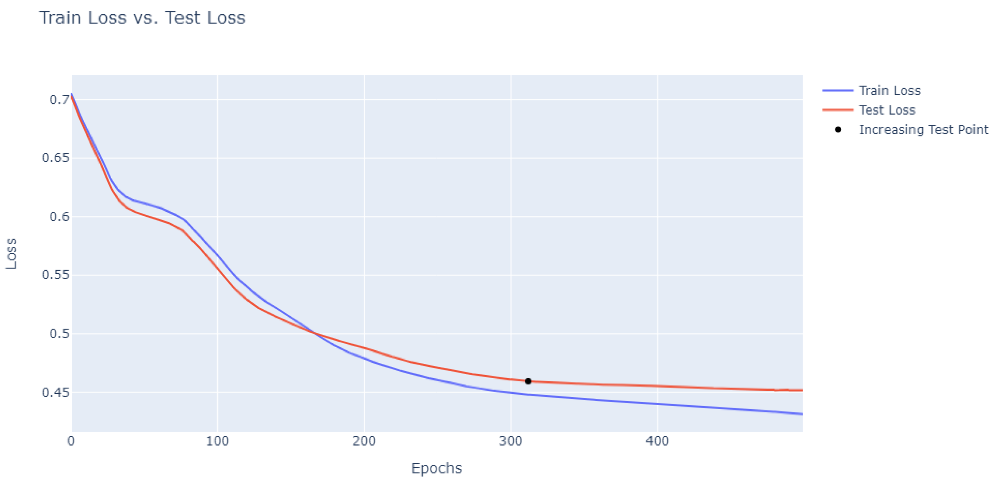
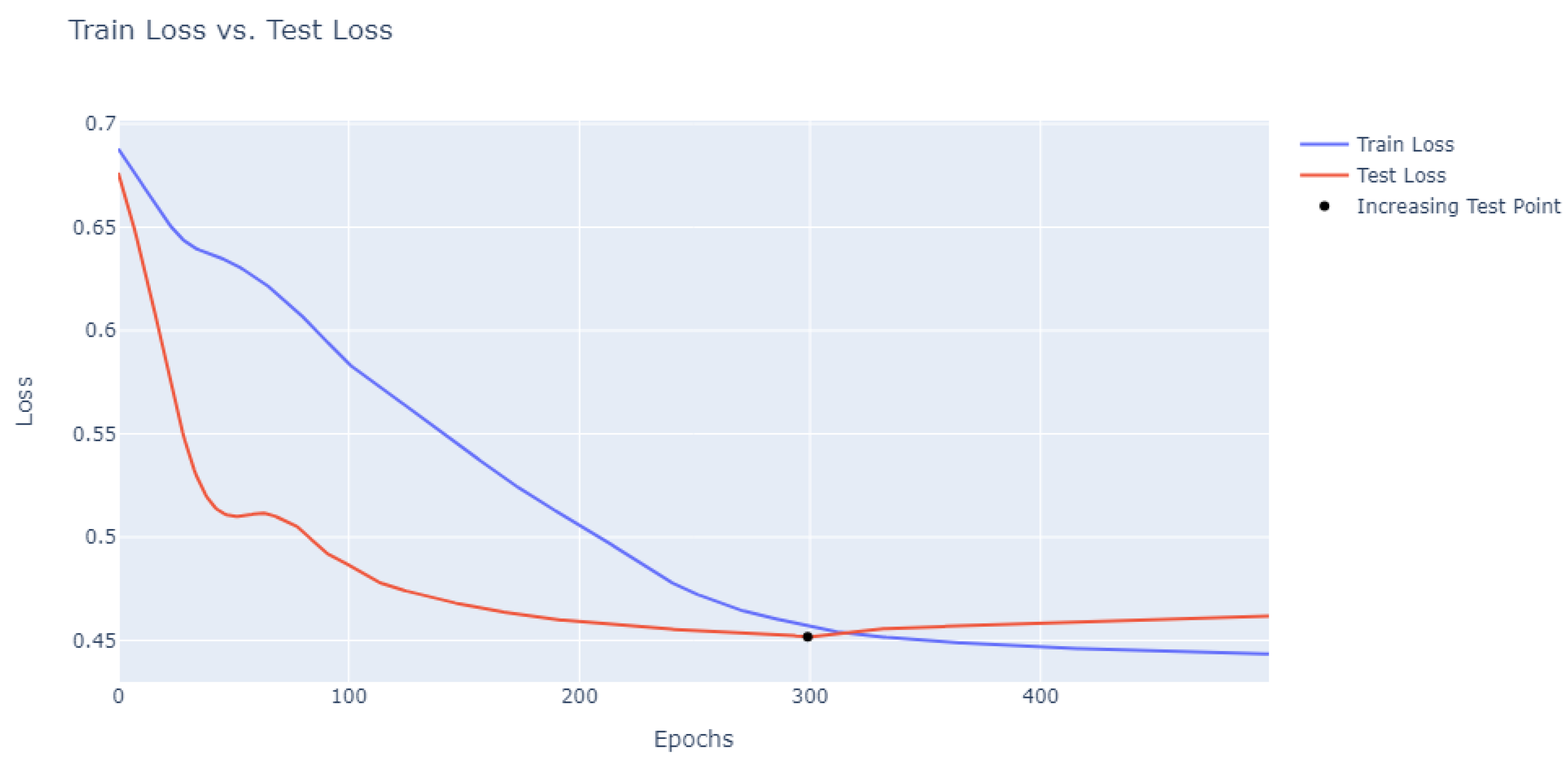
We trained the model using the cross-entropy loss function, which is particularly suited for classification problems. The adaptive moment estimation (Adam) optimizer was chosen for its efficiency and ability to handle large datasets [22], with a learning rate of 0.002. The training was carried out over 300 epochs (Figure 6 and Figure 7) to ensure a robust model that can handle the complexity of the 100 < input parameters and 10,000 < data points.

We carefully chose the architecture of this model to address the specific challenges of this task. The use of ReLU activation functions allows the model to learn non-linear relationships, which are expected given the complex nature of audio signals [23]. The multiple layers enable the model to learn hierarchical representations of the input features, which is crucial given the large number of input parameters.

The selection of the Adam optimizer was primarily influenced by its efficiency, its popularity in state-of-the-art machine learning applications, and its robustness in handling local convergence. While the dataset size is not exceptionally large (<5000), the task is complex due to the 26 input parameters and the challenge of recognizing patterns in 10-s audio segments, which are considerably longer than those typically used in other noise detectors. For example, as cited in the related works section [14], the focus is often on detecting noises that last for fractions of a second. In contrast, our goal is to predict the quality of audio-to-text transcriptions, for which a 10-s audio segment is actually quite short. Therefore, the architecture of this model is designed to strike a balance between computational efficiency and the specific complexities associated with audio quality classification.

4. Results

The ‘Results’ section of the paper is organized into two main subsections: ‘Training Results’ and ‘Implementation Results’. The ‘Training Results’ portion details the overall performance metrics of the model, comparing them against a test set that has been categorized into two binary groups: ‘Acceptable’ and ‘Not Acceptable’. Meanwhile, the ‘Implementation Results’ subsection focuses on evaluating the performance of an automated transcriber, both with and without the incorporation of the trained filter, as judged by human observation.

4.1. Training Results

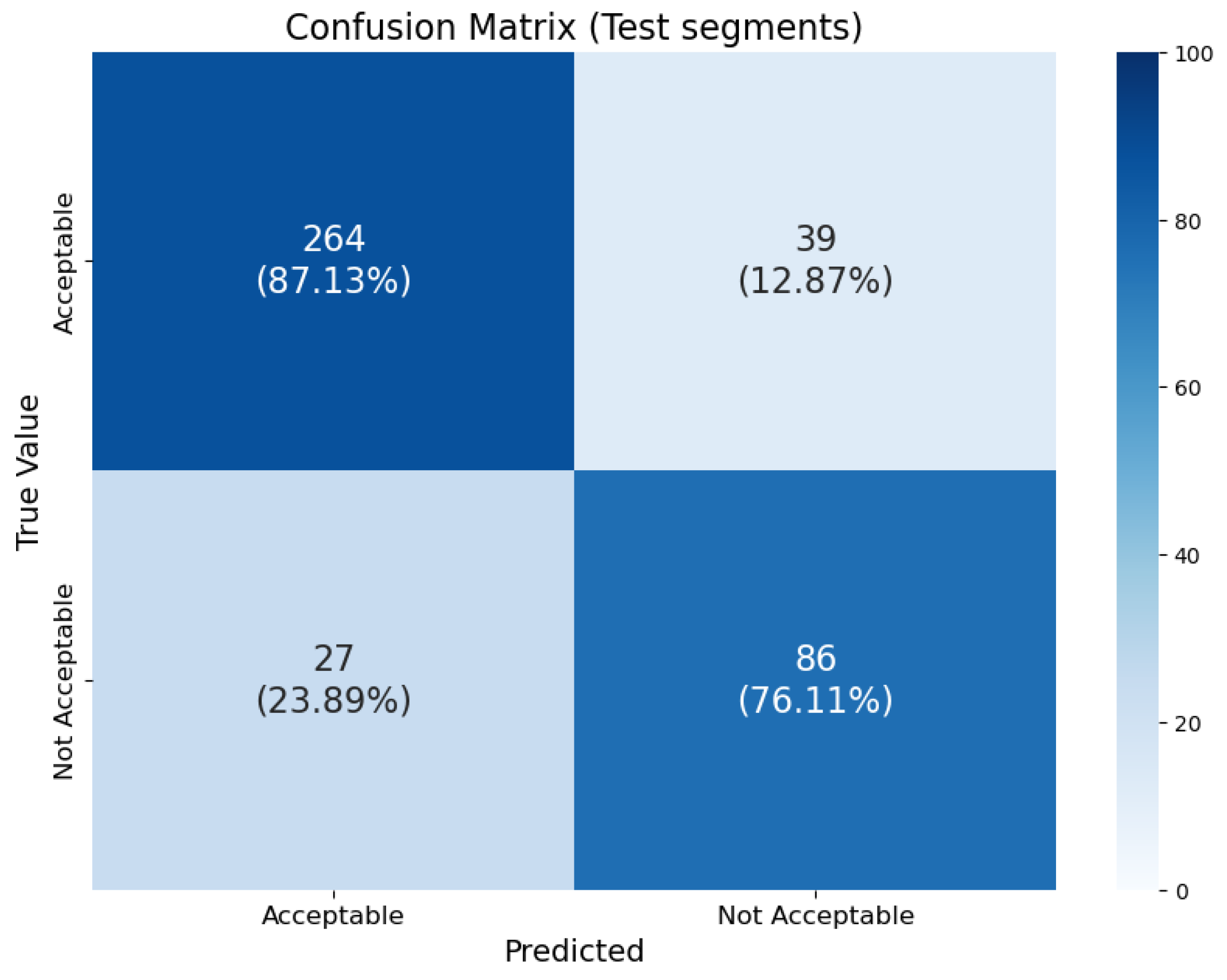
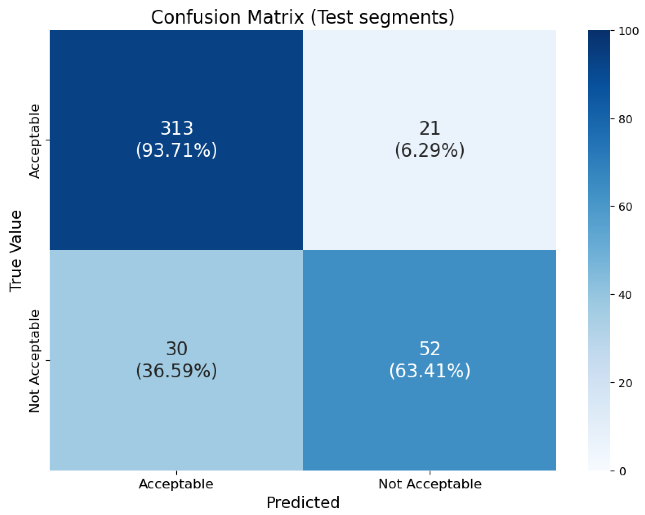
We employed two different data splits for training and testing. In the first split, we randomly divided the data without specific separation criteria, using 80% (1512 segments) for training and the remaining 20% (378 segments) for testing. We did not train the model on this test data. For the second, more manual split, we ensured that the 378 testing segments came from entirely different teaching sessions than the 1512 training segments. We chose this deliberate separation for two main reasons: first, to avoid testing on “duplicated” segments that the model had already seen during training, and second, to evaluate the model’s performance with new teaching sessions, distinct voices, varied dynamics, and other unique characteristics.

To further ensure the accuracy and reliability of our model’s predictions, we employed a human classifier to test on teaching sessions not included in either the training or testing sets. We will present and discuss the results of both the automated and human classifications in the subsequent sections.

4.1.1. Metrics of the Training Results

The area under the curve (AUC) is a metric that provides an aggregate measure of a model’s performance across all possible classification thresholds. It is particularly useful for binary classification problems, as it evaluates the model’s ability to distinguish between the “Acceptable” and “Non Acceptable” classes. In the context of the provided code, the AUC was calculated using the roc_auc_score function from the sklearn.metrics module.

To compute the AUC, the true labels and the probability scores for the “Non Acceptable” class were used. Specifically, the probability scores for the “Non Acceptable” class were extracted from the y_pred_train and y_pred_test tensors. These extracted scores, along with the true labels, were then passed to the roc_auc_score function to obtain the AUC values for both the training and test sets.

In the evaluation process of the classification model, several performance metrics were computed using the probability scores and the true labels. These probability scores, generated by the model, represent the likelihood of an instance belonging to a particular class. These scores were then converted into predicted classes using a threshold of $0.5$. From the predicted classes and the true labels, true positive(s) ($TP$), false positive(s) ($FP$), true negative(s) ($TN$), and false negative(s) ($FN$) were computed for both the training and test datasets.

The performance metrics were defined as follows:

$$\begin{array}{cc}\hfill \mathrm{Precision}& =\frac{TP}{TP+FP}\hfill \\ \hfill \mathrm{Accuracy}& =\frac{TP+TN}{TP+TN+FP+FN}\hfill \\ \hfill \mathrm{Recall}& =\frac{TP}{TP+FN}\hfill \\ \hfill \mathrm{F}1\mathrm{Score}& =2\times \frac{\mathrm{Precision}\times \mathrm{Recall}}{\mathrm{Precision}+\mathrm{Recall}}\hfill \end{array}$$

The results of the model metrics in the test sample are shown in Table 2 and Figure 8 and Figure 9.

As mentioned in Section 3.5 we explored the use of balancing techniques to evaluate in a balanced test set. From this balancing, we calculated the metrics in Table 3 and Table 4.

4.2. Implementation Results

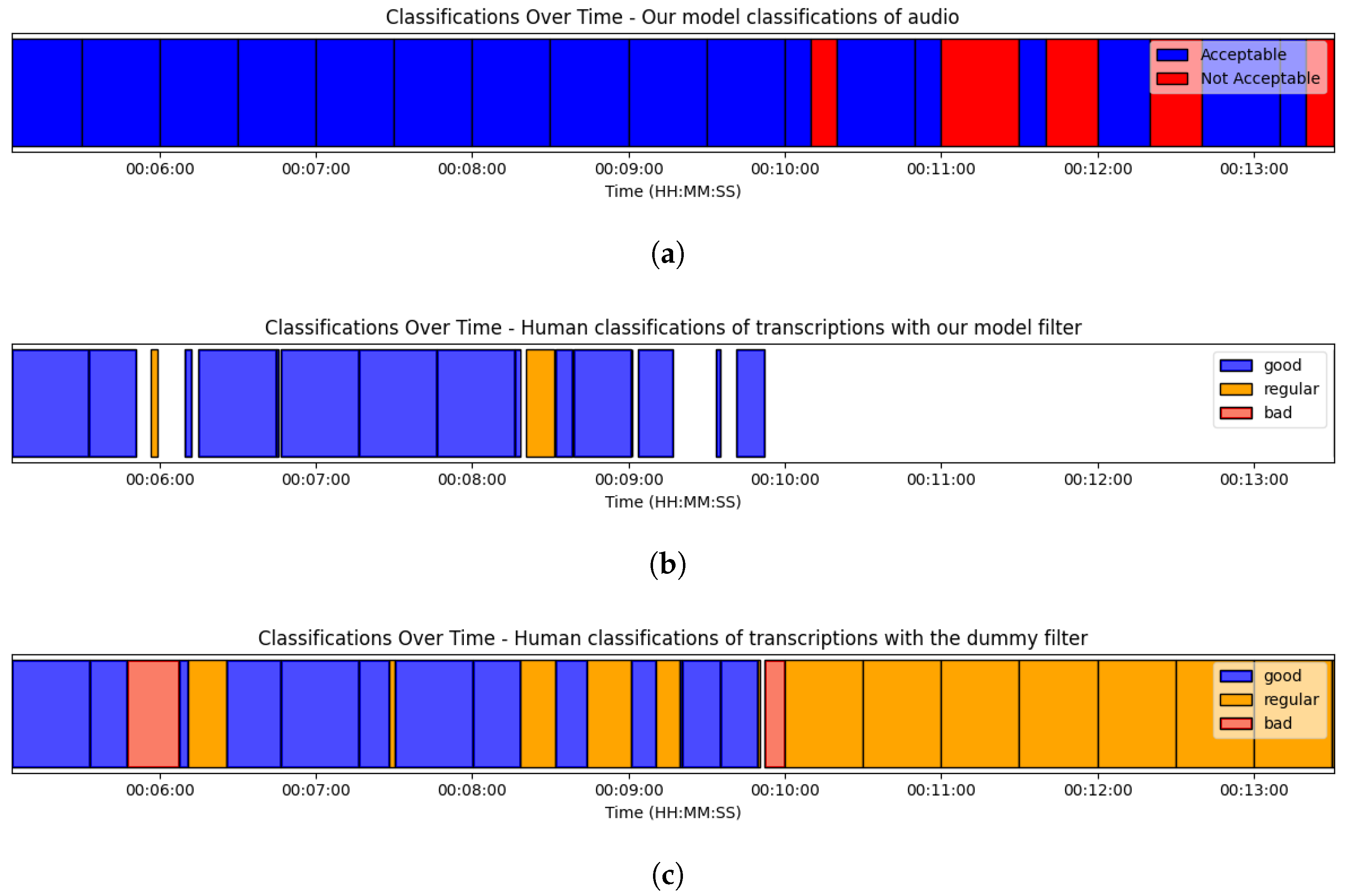
To evaluate the model’s effectiveness in enhancing transcription quality, three classes were transcribed using both our tool and a dummy model. Subsequently, a human evaluator assessed the transcription quality at various intervals throughout each class. We instructed the evaluator to label the transcription as “Good” if the automatic transcriber’s output was accurate, “Regular” if there were minor errors, and “Bad” if the transcription bore little to no resemblance to the audio segment. Only transcribed segments underwent this classification.

The human evaluator labeled the transcriptions at consistent time intervals for both models. The dummy model predicts every transcription as “acceptable”, akin to using the Whisper transcriber without any filtering. In contrast, our model filters out the “Not acceptable” labels based on the trained neural network’s predictions.

We tallied the number of “Good”, “Regular”, and “Bad” transcriptions, and the results are presented in the subsequent table.

There are two primary reasons some audio segments lack transcription. Firstly, the Whisper transcriber sometimes determines that certain audio portions do not contain transcribable content. Secondly, our model’s filter instructs the Whisper transcriber not to transcribe specific segments. The following image (Figure 10) illustrates how our model’s filter impacts transcriptions and human labels. For comparison, we also provide an image showcasing the transcription without our filter, termed the “dummy model”.

The following tables (

Table 5. Comparison between our model and the dummy model for Class 1.

Teaching Session 1
Label	Time (HH:MM:SS)	Percentage of Transcription	Total Percentage
the dummy:
Good	00:04:08.23	51.61%	47.14%
Regular	00:01:12.71	15.12%	13.81%
Bad	00:02:40.04	33.27%	30.39%
No transcription	00:00:45.63		8.66%
Total	00:08:46.62		100.0%
our model:
Good	00:04:15.62	93.12%	48.54%
Regular	00:00:14.07	5.13%	2.67%
Bad	00:00:04.82	1.76%	0.92%
No transcription	00:04:12.12		47.87%
Total	00:08:46.63		100.0%

,

Table 6. Comparison between Our Model and the Dummy Model for Class 2.

Teaching Session 2
Label	Time (HH:MM:SS)	Percentage of Transcription	Total Percentage
the dummy:
Good	00:07:07.85	54.34%	53.92%
Regular	00:05:31.97	42.16%	41.84%
Bad	00:00:27.55	3.5%	3.47%
No transcription	00:00:06.04		0.76%
Total	00:13:13.44		100.0%
our model:
Good	00:05:00.35	91.16%	37.85%
Regular	00:00:29.12	8.84%	3.67%
Bad	00:00:00.00	0.0%	0.0%
No transcription	00:07:43.95		58.47%
Total	00:13:13.43		100.0%

and

Table 7. Comparison between our model and the dummy model for Class 3.

Teaching Session 3
Label	Time (HH:MM:SS)	Percentage of Transcription	Total Percentage
The dummy
Good	00:13:16.33	91.16%	86.83%
Regular	00:00:25.01	2.86%	2.73%
Bad	00:00:52.17	5.97%	5.69%
No transcription	00:00:43.55		4.75%
Total	00:15:17.06		100.0%
Our model
Good	00:12:21.01	99.73%	80.8%
Regular	00:00:02.00	0.27%	0.22%
Bad	00:00:00.00	0.0%	0.0%
No transcription	00:02:54.06		18.98%
Total	00:15:17.08		100.0%

) show the results of the human ratings on all audio segments of each teaching session comparing our filter with the dummy filter, the Time column displays the total sum of segment durations grouped according to the label assigned by the human classifier based on how well the transcription matched the audio. The No Transcription row represents the sum of segments that were not labeled due to the absence of a transcription. The Percentage of Transcription column considers 100% as the sum of the times of segments that have an assigned transcription. Meanwhile, the Total Percentage column considers the entire audio duration, including those segments without an assigned transcription, as 100%:

First and foremost, we aim to gauge whether our filter is inadvertently causing any “harm”—that is, filtering out segments that should rightfully be categorized as “Good”. In the ideal scenario, the total percentage of “Good” segments from the filtered data should align closely with the “Good” percentage from the dummy model, which underwent no filtration. To ascertain this, we conducted a Z-test for each teaching session, and the outcomes of these tests are presented below (

Table 8. The hypothesis is that the total percentage of the dummy model is equivalent to the total percentage from our model.

	(Z-Tests)
Lecture	Z-Value	p
1	−0.15	0.5309
2	7.23	5.01 × 10${}^{-13}$
3	3.64	2.71× 10${}^{-4}$

):

From the table, it is evident that for teaching session 1, the difference between our model and the dummy model is not statistically significant, with a p-value of 0.5309 This implies that our filter performs comparably to the dummy model for this class, not omitting a notable number of “Good” segments. However, for teaching session 2 and teaching session 3, the differences are statistically significant with p-values of 5.01 × 10${}^{-13}$ and 2.71 × 10${}^{-4}$, respectively. This indicates that our model is likely excluding a significant number of segments that should have been categorized as “Good” for these lectures. This provides evidence that, at least for lectures 2 and 3, the filter in our model might be causing inadvertent “harm” by misclassifying or omitting segments that in the dummy model are identified by the human classifier as “Good”.

Having previously assessed the level of “harm” our filter may have caused by potentially omitting segments that should have been categorized as “Good”, we now shift our focus to measure its efficacy. Specifically, we aim to determine how well our filter managed to exclude segments that indeed should have been filtered out. Assuming each measurement as independent, we conducted a two-sided Z-test for proportions of individual categories, and we performed a chi-squared test for overall model comparison, yielding the following results (

Table 9. Hypothesis test results. For the Z-tests, a positive value suggests that the dummy model has a higher percentage in that category, whereas a negative value indicates the opposite. A p-value less than 0.05 indicates a statistically significant difference between the two models.

	(Z-Tests Good)		(Z-Tests Regular)		(Z-Tests Bad)		(${\mathit{\chi }}^2$ Overall)
Lecture	Z-Value	p	Z-Value	p	Z-Value	p	p
1	−6.5624	5.29 × 10${}^{-11}$	2.3417	0.0192	5.8619	4.58 × 10${}^{-9}$	1.55 × 10${}^{-10}$
2	−5.8475	4.99 × 10${}^{-9}$	5.4056	6.46 × 10${}^{-8}$	1.8874	0.0591	3.09 × 10${}^{-8}$
3	−2.9063	3.66 × 10${}^{-3}$	1.4755	0.1401	2.4807	0.0131	0.0143

).

For teaching session 1, the negative Z-value in the ‘Good’ category indicates that our model had a better performance, achieving a higher “Good” percentage than the dummy model. Conversely, the positive Z-values in both the ‘Regular’ and ‘Bad’ categories suggest that our model had a lower percentage in these categories, indicating a better performance compared to the dummy model.

For teaching session 2, the negative Z-value in the ‘Good’ category indicates that our model had a better performance. The positive Z-values in both the ‘Regular’ and ‘Bad’ categories suggest that our model had a lower percentage in these categories, indicating a better performance compared to the dummy model. However, the ‘Bad’ category’s p-value indicates that this difference is not statistically significant.

For teaching session 3, the negative Z-value in the ‘Good’ category indicates that our model had a better performance. The positive Z-value in the ‘Bad’ category suggests that our model had a lower “Bad” percentage, indicating a better performance. However, the ‘Regular’ category did not show a statistically significant difference between the two models.

Overall, the chi-squared tests further support these findings, indicating a significant difference in performance between our model and the dummy model across all three lectures.

4.3. Suppression of Hallucinations in Transcripts

In the introductory chapter, we discussed the issue of hallucinations generated by automatic transcribers and how they could emerge in unexpected situations, contaminating any data obtained from the text. We employed our filter specifically to gauge the impact on hallucinations.

From the classroom recordings exposed in the results, we proceeded to evaluate the number of hallucinations, measured in terms of words obtained from these same recordings transcribed with our filter. The results of this evaluation can be seen in

Table 10. Number of words representing automatic transcriber hallucinations in class sessions with varying audio quality.

Lecture	Duration	Word Count (Segment)	Word Count (Hallucination)	Percentage
1	01:18:40	3668	119	3.24%
2	01:19:26	4309	3	0.07%
3	01:26:10	8989	38	0.42%

and

Table 11. Number of words representing automatic transcriber hallucinations in class sessions with varying audio quality, following the post-application of our model’s filter.

Lecture	Duration	Word Count (Segment)	Word Count (Hallucination)	Percentage
1	01:18:40	2175	22	1.01%
2	01:19:26	4281	0	0.00%
3	01:26:10	7191	0	0.00%

.

5. Discussion

The obtained results provide a detailed insight into the performance of our model compared to a dummy model across different scenarios. We will discuss these findings in detail below.

5.1. General Analysis of the Results

Upon examining the three classes, it is evident that each presents distinct characteristics in terms of transcription quality. In teaching session 1, the audio quality is at extremes, with a significant proportion of both “Good” and “Bad” transcriptions, and a smaller proportion of “Regular”. teaching session 2, on the other hand, displays a high proportion of “Good” and “Regular” transcriptions, with almost none being “Bad”. Finally, teaching session 3 stands out for having exceptionally high audio quality, with a vast majority of “Good” transcriptions and very low proportions of “Regular” and “Bad”. These differences, confirmed qualitatively by a human classifier, allow us to delve deep into the behavior of our model across different contexts.

5.2. Effect on Hallucinations

We addressed the issue of hallucinations in transcripts, representing inaccuracies introduced during automatic transcription. Our filter’s impact is evident in Table 10 and Table 11.

Initially, transcripts exhibited hallucinations ranging from 0.07% to 3.24%. These variations underscore the unpredictable nature of hallucination occurrence in automatic transcriptions.

Post-filter application, hallucination percentages reduced, often reaching zero, indicating the filter’s effectiveness in suppressing these inaccuracies. However, it is important to note that the distribution of hallucinations was not uniform across all scenarios. In cases with challenging audio environments, some hallucinations persisted despite the filter’s application.

This distribution highlights the filter’s context-dependent performance. While it excels in favorable audio conditions, further improvements are needed for extreme cases. This nuanced understanding underscores the importance of considering the specific audio quality when implementing such filters in practical applications.

5.3. Damage Control

One of the primary goals in developing our filter was to ensure it did not cause “harm” by filtering out segments that should be transcribed correctly. The Z-test results indicate that, in general, our filter tends to perform better in classes where there is a clear contrast between “Good” and “Bad” transcriptions. However, in classes like teaching session 2, where there is a mix of “Regular” and “Good” transcriptions, the filter tends to make more mistakes in filtering out segments that could have been transcribed correctly.

This suggests that the model struggles to distinguish between “Good” and “Regular” transcriptions in scenarios where the errors are minor and more subtle. In such cases, the model tends to be more conservative and filters out segments that might have been transcribed correctly.

5.4. Benefits of Using the Filter

Despite the aforementioned limitations, it is evident that our filter offers significant benefits in terms of improving the overall quality of transcriptions. In classes where there is a high proportion of “Bad” transcriptions, like teaching session 1 and Teaching session 2, the filter is capable of significantly improving the proportion of “Good” transcriptions. However, in classes like teaching session 3, where there are very few “Bad” segments to filter out, the benefit is less pronounced.

It is crucial to consider how the Whisper transcriber works and how the segments are labeled. Given that Whisper uses 30-s chunks for transcription and can base itself on the text from the previous chunk, erroneous transcriptions in one chunk can negatively impact subsequent transcriptions. This cumulative effect can have a significant impact on the overall quality of transcriptions [6].

6. Conclusions

In addressing our first research question regarding the enhancement of information acquisition by eliminating interferences and noises, we found that it is indeed feasible to improve transcription quality in elementary school classrooms. Importantly, this can be achieved without a significant budget. Our study demonstrates that modern technology, specifically neural network-based filters applied to small audio samples (3–5 h), can effectively enhance the quality of noisy transcriptions. This is particularly significant as it negates the need for high-end sound equipment and does not disrupt the normal operation of a classroom. The use of an affordable UHF microphone transmitting to a smartphone located 8 m away has proven to be adequate for this purpose.

Addressing our second research question about ensuring valuable information is not inadvertently filtered out, we recognize that one of the primary challenges of our model is the non-negligible number of potential good-quality transcriptions that are lost. This is due to the misprediction of good-quality audio being labeled as poor quality.

Regarding areas of improvement, our filter model performs commendably but could benefit from an expanded dataset. This suggests that the extent to which we can ensure valuable information is not inadvertently filtered out could be further optimized by increasing the variety and quantity of data used for training.

One of the biggest challenges of the model is the non-negligible number of potential good-quality transcriptions that are lost due to the poor prediction of good-quality audio being labeled as poor quality.

In the future, we anticipate improved versions of this model, which will not only allow us to enhance the transcriptions but also perform other related tasks, such as improving speaker diarization, for research purposes like detecting the activity of teachers and/or students in the classroom. Additionally, we plan to implement state-of-the-art solutions to further refine our approach. This will enable us to conduct a comprehensive comparison between the performance of these advanced methods and our current model, thereby offering a more robust and efficient solution for the challenges faced in educational research settings.

Additionally, there is a growing interest in applying our filter to other automatic transcription systems specifically tailored for classroom environments, such as the one developed by [24]. This transcriber has shown to be particularly suited for classroom settings, demonstrating robustness against ambient sounds and the specific discourse style of teaching. By enhancing the quality of transcriptions produced by such systems, we could facilitate more accurate analyses of teacher discourse. This, in turn, would bolster efforts to classify and understand teaching practices, like those detailed in [25], which leverage acoustic features to identify pedagogical activities in the classroom as per protocols like COPUS [26], a protocol that is uniquely designed to depend minimally (if at all) on the classifier’s subjective interpretations of ongoing classroom activities. As such, it holds significant potential as a protocol for automated classification. In summary, merging efficient filtering technologies with specialized automatic transcriptions could revolutionize the way we analyze and comprehend classroom dynamics, providing potent tools for both researchers and educators alike.