Figure 1.
Photoacoustic principle and the photoacoustic setup utilized for experimentation in the study. (a) A block diagram that shows the major steps involved in the photoacoustic imaging data acquisition, starting from laser actuation to photoacoustic image reconstruction. (b) Schematic diagram of an actual photoacoustic imaging microscopy setup utilized for the actual experimentation in the study.
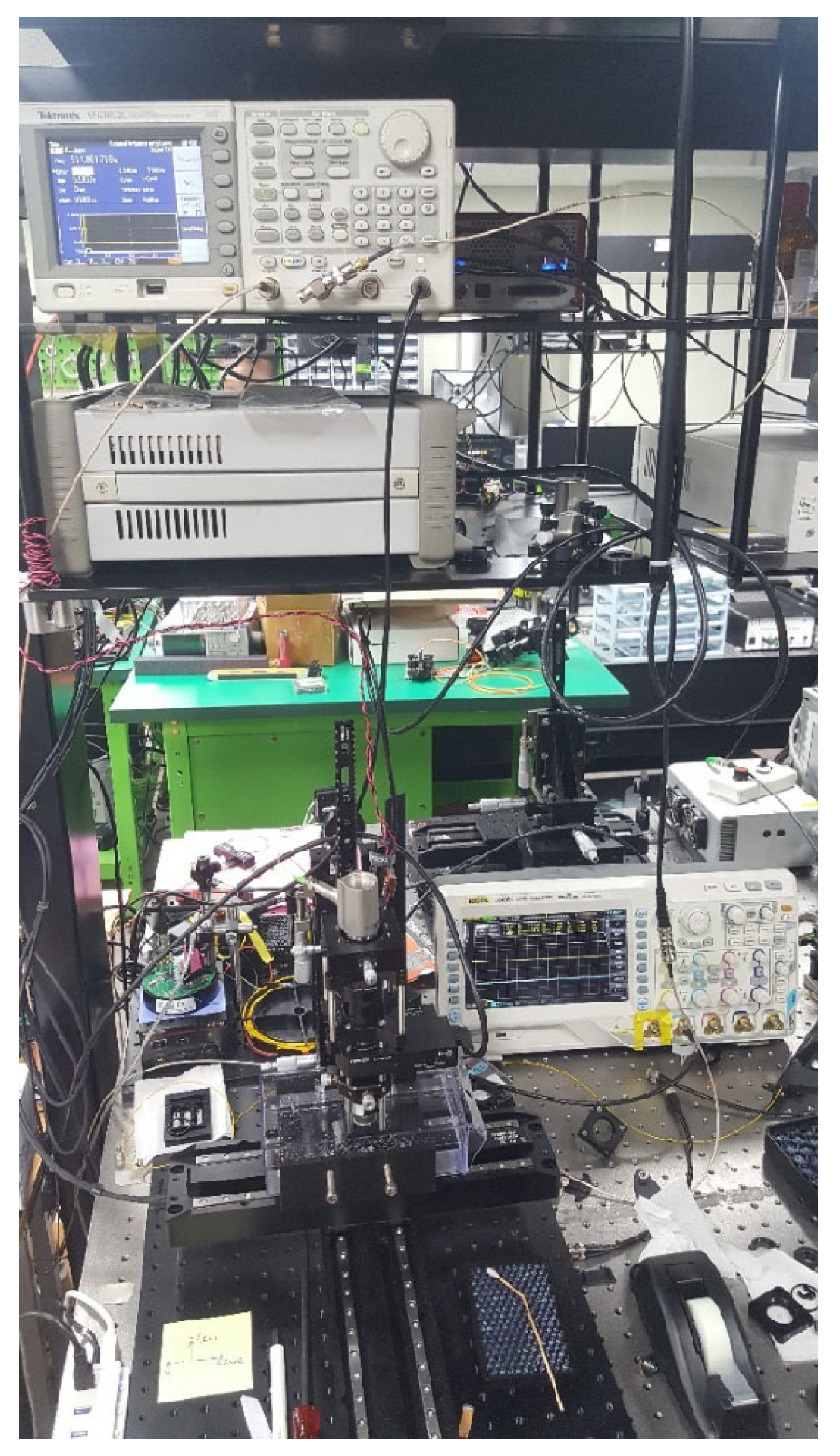
Figure 2.
Actual picture of the PAM setup utilized for experimentation.
Figure 2.
Actual picture of the PAM setup utilized for experimentation.
Figure 3.
Steel samples used for actual PAI experimentation are presented in the first column; the second column provides a few example PA images reconstructed from the acoustic responses received after experimentation. Finally, the third column shows a few images after application of data augmentation techniques.
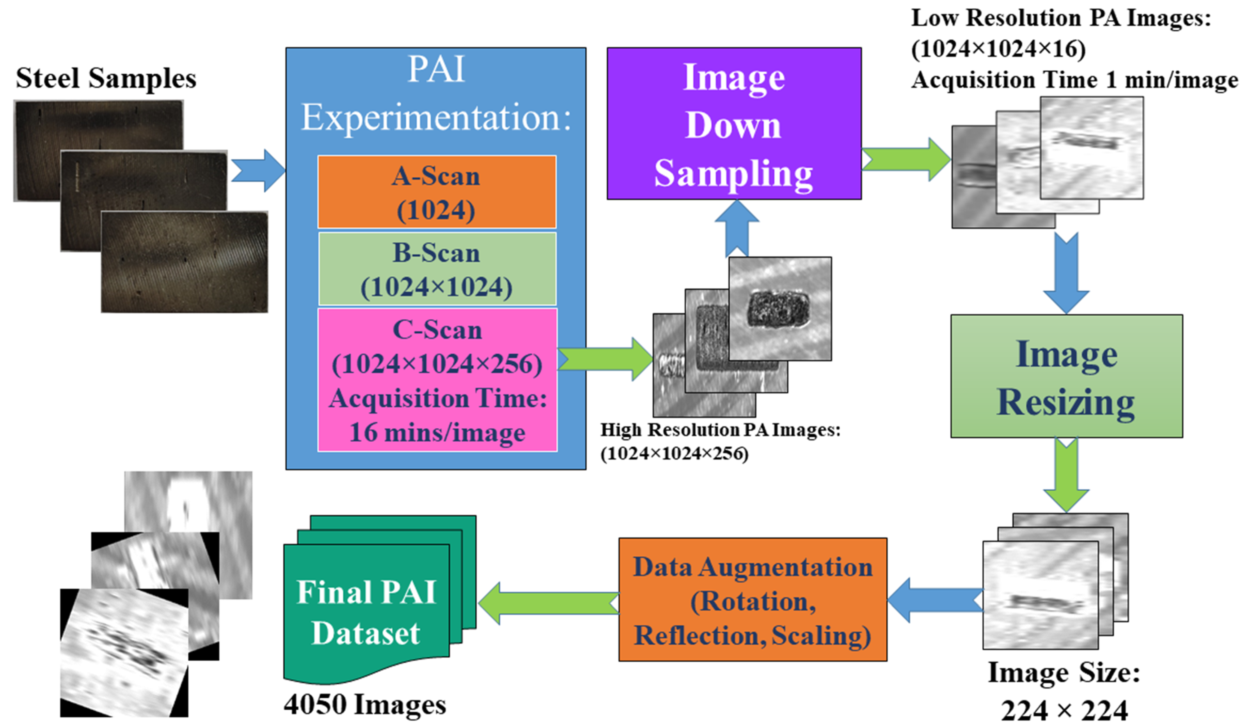
Figure 4.
Overall scheme showing the steps involved in the construction of the final PAI dataset starting from PAI experimentation, image preprocessing, image resizing, and data augmentation.
Figure 4.
Overall scheme showing the steps involved in the construction of the final PAI dataset starting from PAI experimentation, image preprocessing, image resizing, and data augmentation.
Figure 5.
Schematic diagram for combinatorial application of deep CNN models for feature extraction, PCA for dimensionality reduction, and machine learning regression models to predict crack length and width.
Figure 5.
Schematic diagram for combinatorial application of deep CNN models for feature extraction, PCA for dimensionality reduction, and machine learning regression models to predict crack length and width.
Figure 6.
A representation of all the geometries used for simulation. Origin of the coordinate system is the left bottom corner of the steel block. (a) Steel block (dimensions 150 × 50 mm2) without any internal crack. (b) Steel block with a crack (crack width 1 mm height 10 mm) at an offset of (120,0). (c) Steel block with a crack (crack width 10 mm height 1 mm) at an offset of (150,40). (d) Steel block with a crack (crack width 1 mm height 10 mm) at an offset of (30,0). (e) Steel block with a crack (crack width 10 mm height 5 mm) at an offset of (150,40). (f) Steel block with a crack (crack width 10 mm height 5 mm) at an offset of (150,20).
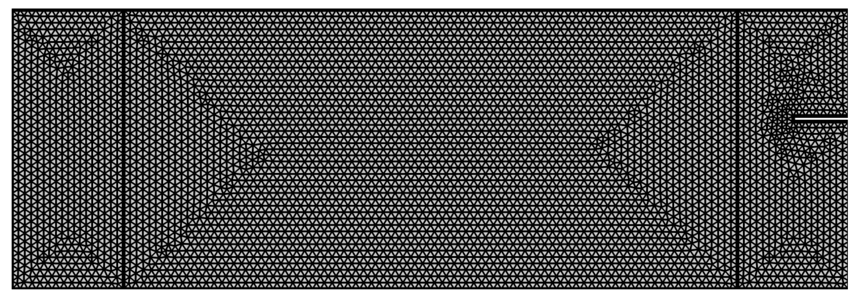
Figure 7.
Geometry details showing the dimension of the steel cylinder, the internal damage, and the approximate mesh size for the numerical analysis.
Figure 7.
Geometry details showing the dimension of the steel cylinder, the internal damage, and the approximate mesh size for the numerical analysis.
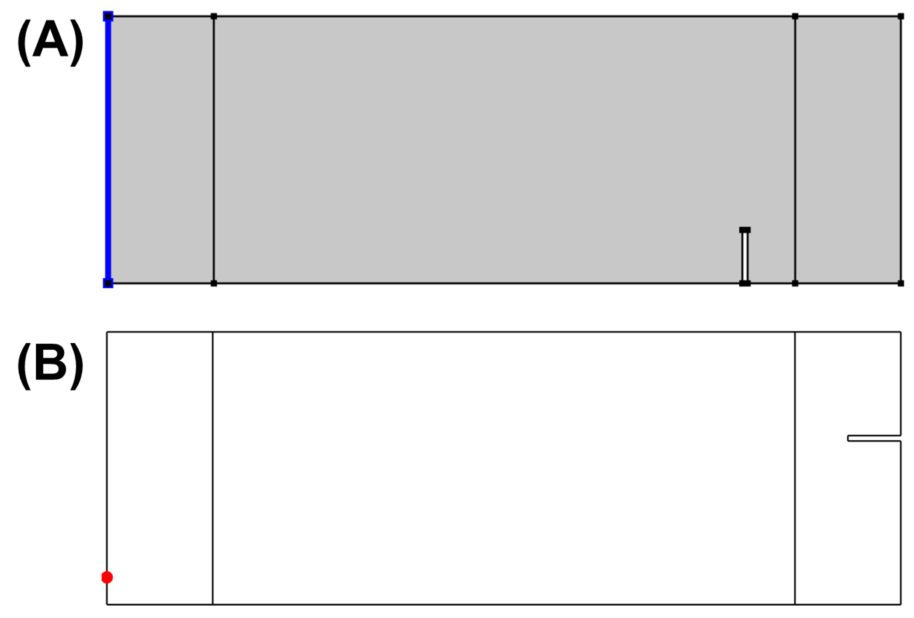
Figure 8.
Actuation point and sensor location set in the simulation. (A) Left face of the geometry is configured as the uniform actuation application area visible as a blue line, (B) Detection point set at a coordinate value of (0, 5), visible as a red dot in the figure.
Figure 8.
Actuation point and sensor location set in the simulation. (A) Left face of the geometry is configured as the uniform actuation application area visible as a blue line, (B) Detection point set at a coordinate value of (0, 5), visible as a red dot in the figure.
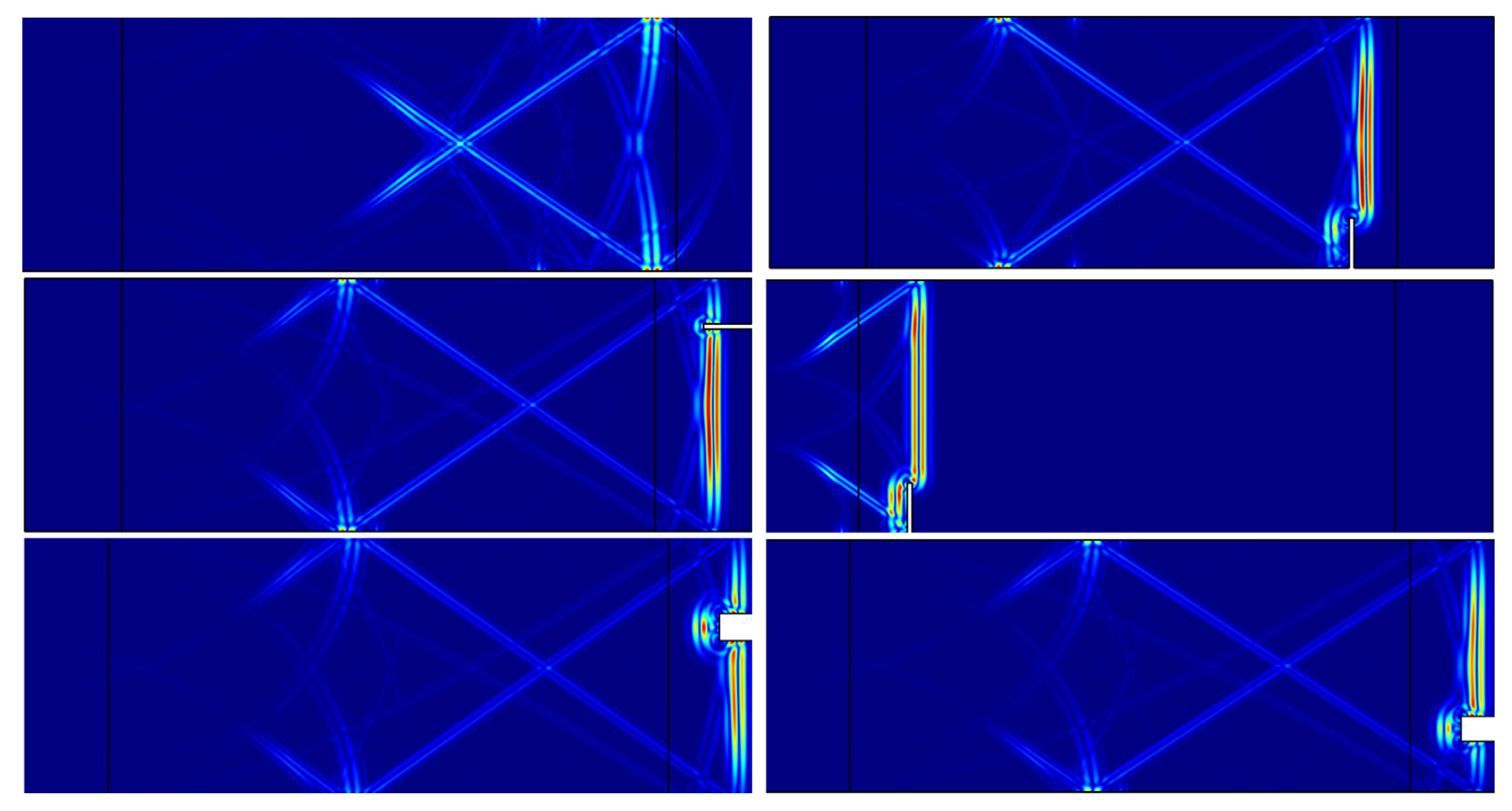
Figure 9.
Simulation snapshot for the propagation of an acoustic wave within samples with internal cracks and without any defect, showing the acoustic wave interaction with internal defects at different locations for all the simulated geometries.
Figure 9.
Simulation snapshot for the propagation of an acoustic wave within samples with internal cracks and without any defect, showing the acoustic wave interaction with internal defects at different locations for all the simulated geometries.
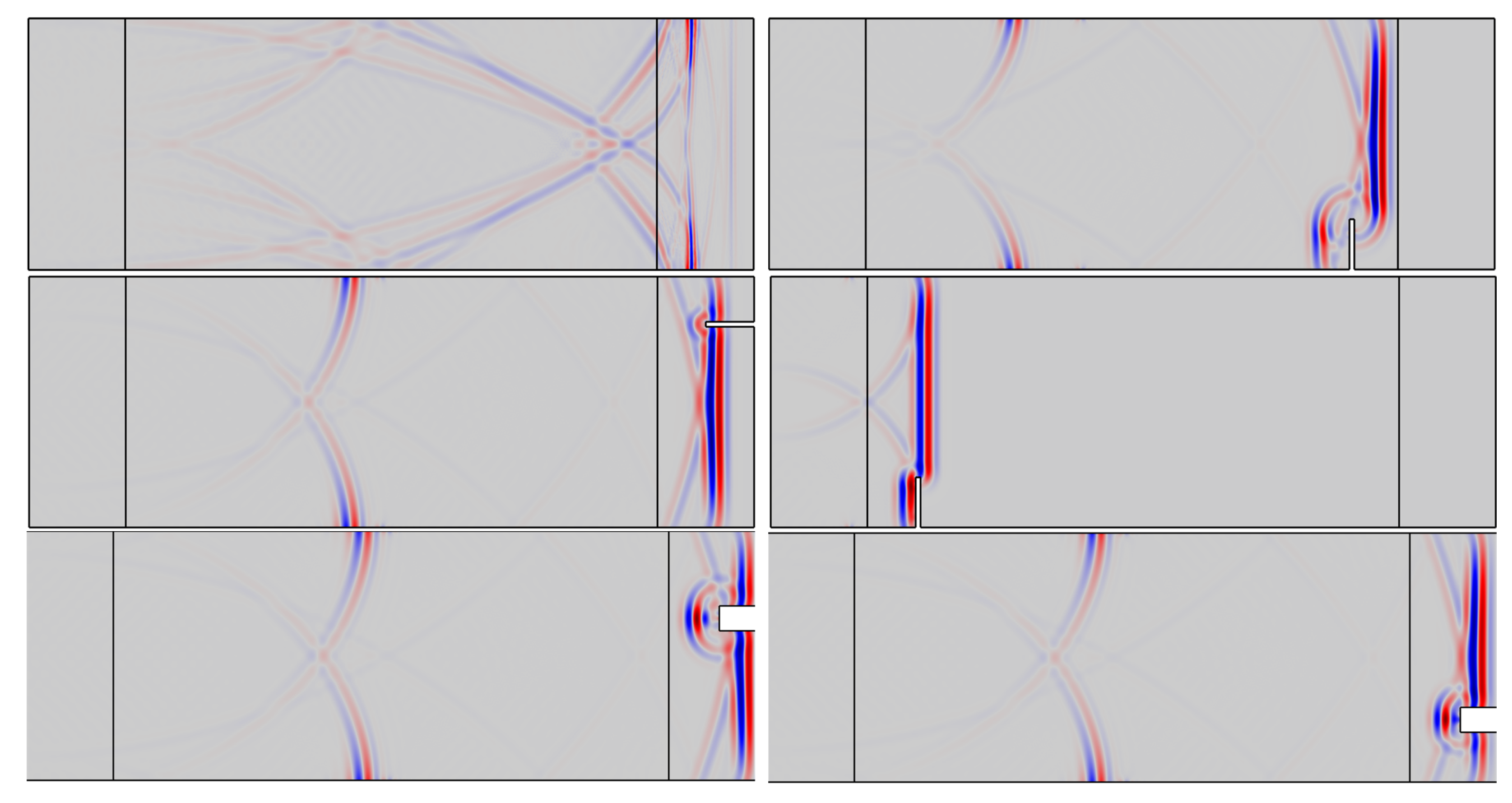
Figure 10.
Simulation snapshot for acoustic pressure of the propagating acoustic wave for all the simulated geometries, showing the reflection and transmission phenomena at the interaction points with internal defects. The red color shows the pressure peaks (compressions), whereas the blue color shows the troughs (rarefactions) of the acoustic wave during propagation.
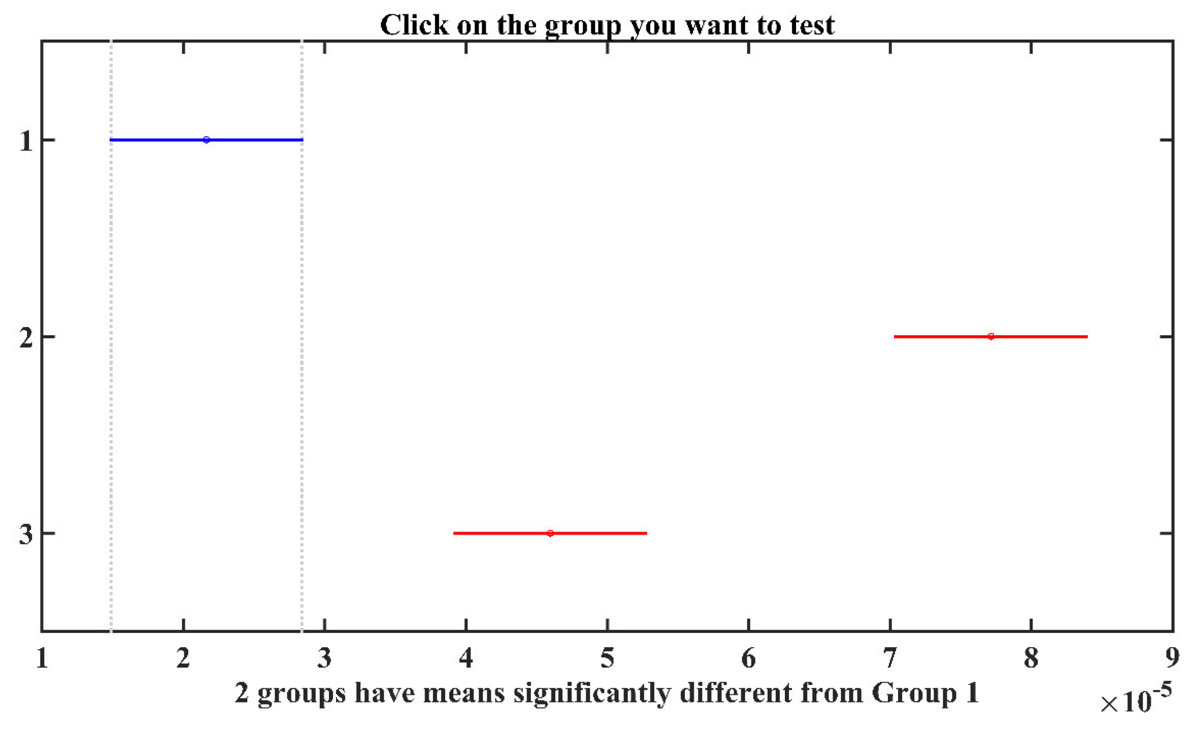
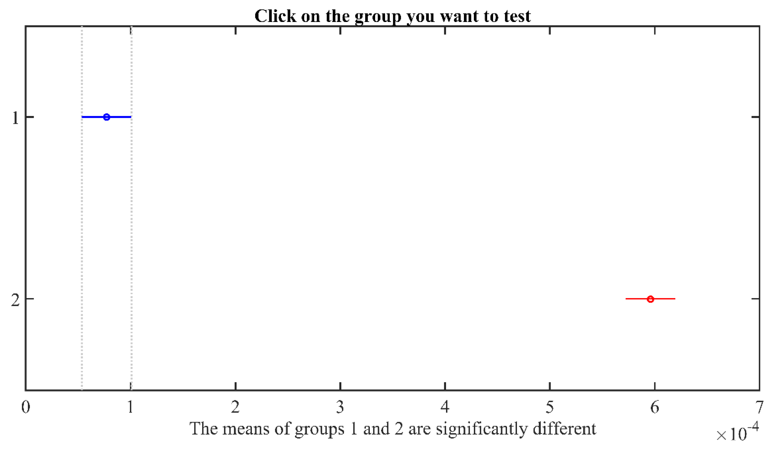
Figure 11.
One-way ANOVA test to compare the means of acoustic responses from a sample with no crack, a crack on the horizontal axis, and crack on the vertical axis to prove statistically that both crack presence and location are distinguishable using a photoacoustic imaging technique. The blue color bar shows that Group 1 is selected.
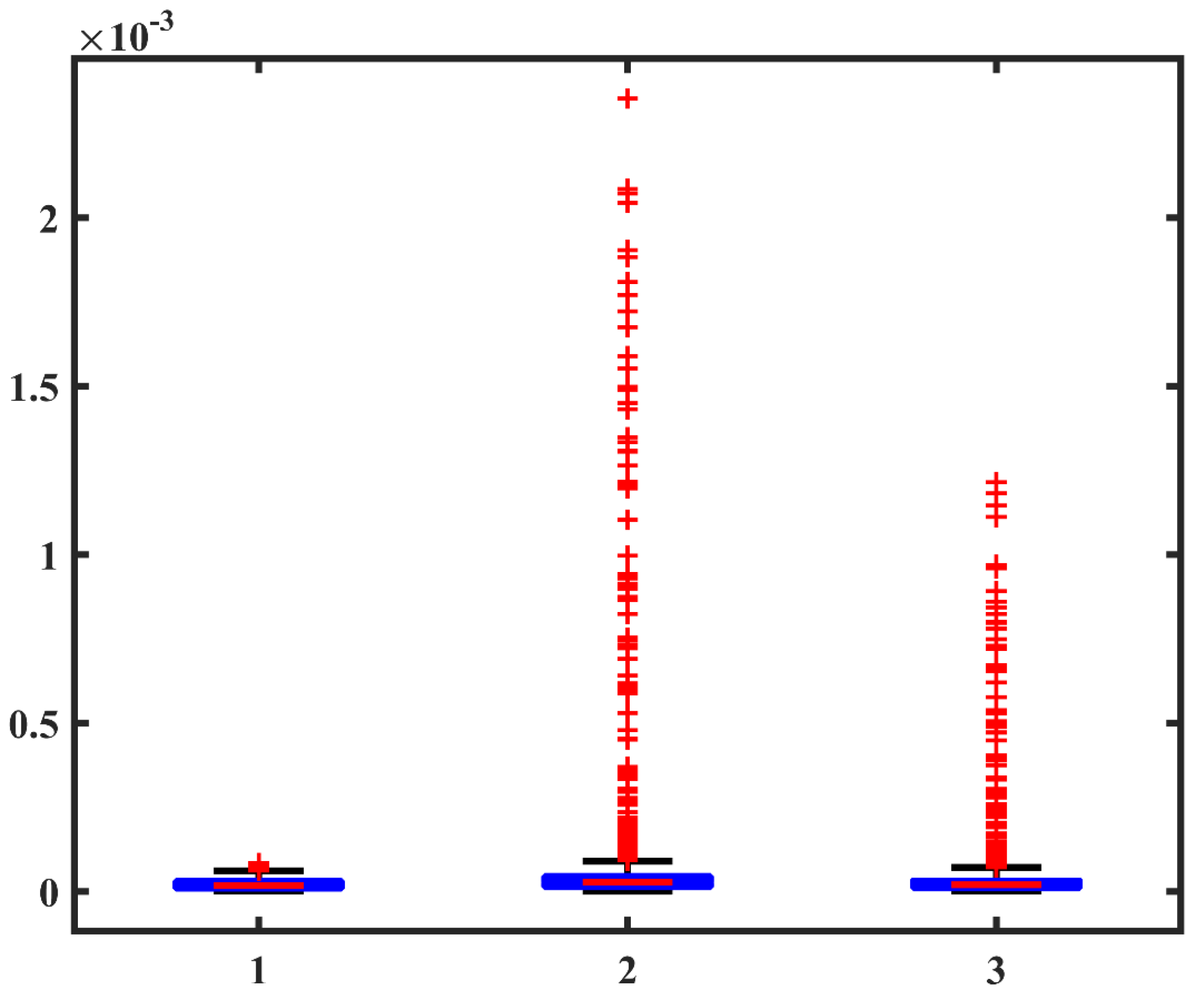
Figure 12.
Box plot showing medians for the one-way ANOVA test to compare the means of acoustic responses from a sample with no crack, a crack on the horizontal axis, and crack on the vertical axis to prove statistically that both crack presence and location are distinguishable using a photoacoustic imaging technique.
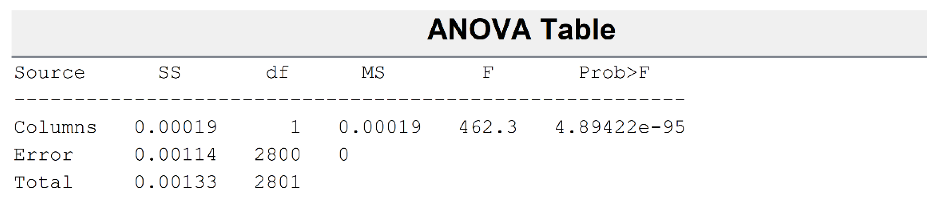
Figure 13.
ANOVA table for the test results of the comparison samples, showing a small p-value < 0.0001 for the one-way ANOVA test to compare the means of acoustic responses from a sample with no crack, a crack on the horizontal axis, and crack on the vertical axis to prove statistically that both crack presence and location are distinguishable using a photoacoustic imaging technique.
Figure 14.
Comparison intervals for the means of the two groups with a crack of the same size but placed at different locations horizontally.
Figure 14.
Comparison intervals for the means of the two groups with a crack of the same size but placed at different locations horizontally.
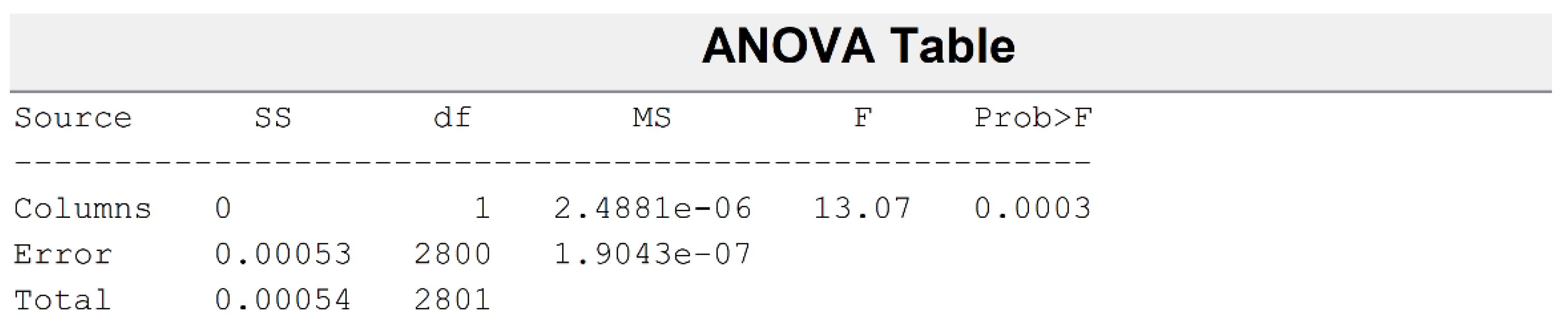
Figure 15.
ANOVA table results in a small p-value (p-value < 0.0001), showing statistically significant differences between the groups being compared with cracks of the same size but at different locations horizontally.
Figure 15.
ANOVA table results in a small p-value (p-value < 0.0001), showing statistically significant differences between the groups being compared with cracks of the same size but at different locations horizontally.
Figure 16.
ANOVA test showing two mutually nonoverlapping intervals for the groups being compared with cracks of the same size but placed at different locations vertically.
Figure 16.
ANOVA test showing two mutually nonoverlapping intervals for the groups being compared with cracks of the same size but placed at different locations vertically.
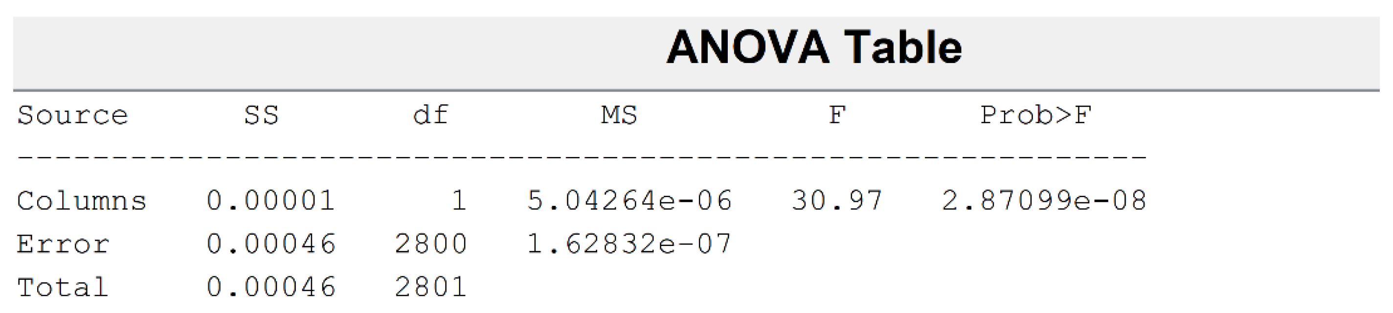
Figure 17.
ANOVA table giving a small p-value (p-value <0.001), showing significant differences among the compared groups with cracks of the same size but at different locations vertically.
Figure 17.
ANOVA table giving a small p-value (p-value <0.001), showing significant differences among the compared groups with cracks of the same size but at different locations vertically.
Figure 18.
One-way ANOVA test showing that the means of both groups have a nonoverlapping interval when comparing samples with internal cracks of different sizes but placed at the same location.
Figure 18.
One-way ANOVA test showing that the means of both groups have a nonoverlapping interval when comparing samples with internal cracks of different sizes but placed at the same location.
Figure 19.
ANOVA table presenting a p-value (p-value < 0.0001) that shows significant differences between the groups being compared; that is, samples with internal cracks of different sizes but placed at the same location.
Figure 19.
ANOVA table presenting a p-value (p-value < 0.0001) that shows significant differences between the groups being compared; that is, samples with internal cracks of different sizes but placed at the same location.
Table 1.
Surface crack dimensions utilized for actual experimentation using the PAM setup to generate raw acoustic response data.
Table 1.
Surface crack dimensions utilized for actual experimentation using the PAM setup to generate raw acoustic response data.
| Crack # | Length (mm) | Width (µm) | Sample Information |
|---|
| 1 | 6 | 300 | Sample 1 |
| 2 | 8 | 300 |
| 3 | 7 | 1000 |
| 4 | 8 | 1000 |
| 5 | 5 | 500 |
| 6 | 1 | 400 | Sample 2 |
| 7 | 8 | 300 |
| 8 | 1 | 350 |
| 9 | 1 | 1000 |
| 10 | 4 | 400 |
| 11 | 2 | 300 | Sample 3 |
| 12 | 4 | 300 |
| 13 | 4 | 500 |
| 14 | 1 | 500 |
| 15 | 1 | 300 |
Table 2.
Total unique images generated by the PAM setup and final images constructed after data augmentation techniques.
Table 2.
Total unique images generated by the PAM setup and final images constructed after data augmentation techniques.
| Attribute | Crack Images |
|---|
| # of cracks | 15 |
| PAM setup’s unique laser excitation angles per crack | 4 |
| Total original images | 15 × 4 = 60 |
| Total Images after applying Data augmentation techniques | 4050 |
Table 3.
Data augmentation techniques and their corresponding parameter values for generating sufficient volumetric data for a deep learning model.
Table 3.
Data augmentation techniques and their corresponding parameter values for generating sufficient volumetric data for a deep learning model.
| Augmentation Technique | Parameters |
|---|
| Rotation | [0, 350] degrees |
| Reflection | X and Y: [−1, 1] |
| Scaling | [0.5, 1] |
Table 4.
Properties of steel material used in the numerical simulation setting.
Table 4.
Properties of steel material used in the numerical simulation setting.
| Description | Value |
|---|
| Density | 7850 kg m−3 |
| Thermal conductivity | 44.5 W/(m·K) |
| Coefficient of thermal expansion | 12.3 × 10⁻⁶ K−1 |
| Bulk velocity | 6200 m s−1 |
| Shear velocity | 3200 m s−1 |
| Young’s modulus | 205 GPa |
| Poisson’s ratio | 0.28 |
Table 5.
The purpose of every comparison carried out is listed along with the geometries involved in the comparison.
Table 5.
The purpose of every comparison carried out is listed along with the geometries involved in the comparison.
| Comp # | Geometries Involved
(Shown in Figure 6) | Purpose (to Show if Statistically Significant Differences Are Present in Acoustic Responses of:) |
|---|
| 1 | 6a, 6b, 6c | |
| 2 | 6b, 6d | 2 samples having internal cracks at two different locations along horizontal axis |
| 3 | 6e, 6f | 2 samples having internal cracks at two different locations along vertical axis |
| 4 | 6c, 6e | 2 samples having internal cracks of different sizes at same location |
Table 6.
RMSE means and standard deviations in the predicted crack lengths (unit: mm) by the CNN model and regression model combinations utilized.
Table 6.
RMSE means and standard deviations in the predicted crack lengths (unit: mm) by the CNN model and regression model combinations utilized.
| | GoogleNet | ResNet50 | VGG16 |
|---|
| Linear regression | 0.91 ± 0.07 | 0.97 ± 0.06 | 0.93 ± 0.05 |
| Support vector regression | 0.81 ± 0.06 | 0.75 ± 0.05 | 0.69 ± 0.05 |
| Random forest regression | 0.79 ± 0.05 | 0.71 ± 0.04 | 0.63 ± 0.03 |
Table 7.
RMSE means and standard deviations in the predicted crack widths (unit: µm) by the CNN model and regression model combinations utilized.
Table 7.
RMSE means and standard deviations in the predicted crack widths (unit: µm) by the CNN model and regression model combinations utilized.
| | GoogleNet | ResNet50 | VGG16 |
|---|
| Linear regression | 9.2 ± 1.2 | 10.1 ± 0.95 | 9.9 ± 0.81 |
| Support vector regression | 7.9 ± 0.75 | 7.3 ± 0.67 | 7.1 ± 0.53 |
| Random forest regression | 7.4 ± 0.63 | 6.9 ± 0.51 | 6.2 ± 0.48 |
Table 8.
ANOVA table with groupwise comparison details.
Table 8.
ANOVA table with groupwise comparison details.
| Group A | Group B | Lower Limit | A-B | Upper Limit | p-Value |
|---|
| 1 | 2 | −6.90 × 10⁻⁵ | −5.55 × 10⁻⁵ | −4.20 × 10⁻⁵ | 9.56 × 10⁻¹⁰ |
| 1 | 3 | −3.78 × 10⁻⁵ | −2.43 × 10⁻⁵ | −1.09 × 10⁻⁵ | 6.84 × 10⁻⁵ |
| 2 | 3 | 1.77 × 10⁻⁵ | 3.12 × 10⁻⁵ | 4.47 × 10⁻⁵ | 1.73 × 10⁻⁷ |


