Improving a Fuel Cell System’s Thermal Management by Optimizing Thermal Control with the Particle Swarm Optimization Algorithm and an Artificial Neural Network

Abstract

The thermal management of proton exchange membrane fuel cell systems plays a significant role in a stack’s lifetime, performance, and reliability. However, it is challenging to manage the thermal system precisely due to the multiple coupling relationships between the stack’s components, its operating environment, and its thermal management system. In addition, temperature hysteresis (temporal inconsistency of temperature with electrochemical reactions and fluid mechanics) imposes more difficulties on thermal control. We aim to develop an effective thermal control model for the fuel cell system to improve the temperature regulation accuracy and response speed and thus achieve highly stable temperature control. A dynamic mechanistic model is first developed based on the physical processes of the stack and its thermal management system. The model is then validated through experiments. Based on this dynamic mechanistic model, a control model is proposed for stack thermal management with the particle swarm optimization algorithm and an artificial neural network. It is applied and compared with the traditional PID algorithm. The simulation results indicate that the regulation time of the coolant inlet temperature as the current changes is reduced by more than 74%, and the overshoot is reduced by more than 50%. Therefore, the control model can enhance the dynamic response capability and temperature control precision under complex operating conditions with constantly changing load current and preset stack temperature, ensuring the temperature’s stability and thus improving the fuel cell system’s reliability and durability.

1. Introduction

Hydrogen energy is one of the most promising clean power sources due to its efficient energy conversion and low carbon emissions. It can sustain diverse resources, the environment, and sustainable development needs in the new era. In the hydrogen energy industry, proton exchange membrane fuel cells (PEMFCs) are widely used in various transportation, industry, and portable energy applications because of their high conversion efficiency, high power density, and lack of pollution [1,2,3,4,5]. Thermal management plays a vital role in the performance of the fuel cell stack. On the one hand, the electrochemical reactions in the stack generate heat. On the other hand, the fuel cell stack has thermal inertia. Multiple coupling relationships exist between the stack and the coolant [6]. Therefore, it is necessary to design an effective thermal management system to maintain the thermal balance of the fuel cell system. The thermal effect can cause operating temperature changes, affecting the proton membrane’s water content, the reaction catalyst’s activeness, and thus the electrochemical reaction rate. Working at an appropriate temperature is conducive to improving the stack’s output performance. When the temperature is excessively high, gas-phase water inside the membrane may leave the stack, causing local drying and even degradation of the electrolyte membrane [7]. On the other hand, if the temperature is too low, the cathode flow channel may be flooded, affecting the oxygen diffusion and increasing the concentration overvoltage, thus reducing the stack’s output performance. It is well known that liquids possess a much higher heat capacity than gases [8], making liquid cooling the most suitable heat exchange method for high-power automotive fuel cell stacks [9]. The liquid cooling of fuel cells requires a reasonable coolant flow field and complex thermal management system support.

A combination of reliable experiments and accurate system models is needed to study thermal management systems. Fang et al. [10] tested a 10 kW fuel cell system and found that the coolant temperature constantly fluctuates with thermal hysteresis, impacting the stack’s performance. To optimize the PEMFC system’s thermal management, multi-dimensional models are studied [11]. Yu et al. [12] developed a 2D thermal model and a thermal management system to simulate the temperature distribution characteristics during stack operation. The results showed that the maximum temperature of the fuel cell is suggested as the representative operating temperature because the maximum temperature can be more conveniently measured and monitored than other possible temperatures. Zhang et al. [13] established a 3D simulation model including fans and radiators and a 1D model to simulate a PEMFC’s cooling system. The results indicate that the 3D simulation can quickly capture fluid flow distribution. In contrast, the simulation time of the 1D thermal system is short, and it can quickly guide the matching of heat transfer components. Thomas et al. [14] combined experiments and a computational fluid dynamic (CFD) model to demonstrate the importance of the thermal conductivity of the fuel cell’s porous layers for analyzing the thermal effects. The strong influence of the temperature profile on water transport through the cell was demonstrated. Rahgoshay et al. [15] simulated serpentine and parallel flow fields with the CFD model, and the results pointed out that heat transfer rate has different effects on different coolant flow fields. Cao et al. [16] proposed a 3D two-phase model to investigate the interaction between water and thermal transport processes. This reveals a coupling relationship between water and thermal management where boundary temperature concurrently affects temperature and water saturation distributions. Although multi-dimensional models can provide high-resolution temperature distributions and accurately reflect the performance, it is impractical to use multi-dimensional models in experiments to improve the thermal management control accuracy and response speed due to high time and computational costs. Therefore, it is necessary to develop high-efficiency mechanistic models that can be applied in real-time control.

Hosseinzadeh et al. [17] developed a zero-dimensional (0D) water and thermal management model. They tested different coolant types and concluded that changing coolant type and temperature can effectively improve the performance of thermal management systems. Nolan et al. [18] established an eighth-order non-linear thermal model of an automotive fuel cell system and constructed a reduced-order model for comparison. The results indicated that the reduced-order model could accurately represent the performance of the non-linear model. Zhao et al. [19] presented a thermal management system model based on electrochemical reactions and thermodynamics, which was validated using the developed experimental system. Their studies can guide the design and optimization of control systems. Liso et al. [20] proposed a control-oriented zero-dimensional (0D) model to investigate temperature variations during load change. Their findings can guide the appropriate coolant mass flow rate and radiator size choices and improve the control capability of the thermal management system. The 0D model has advanced, but components like radiators often lag and overshoot, leading to coolant temperature fluctuation and hysteresis in actual systems. Therefore, combining model and control algorithms is essential [21]. Cheng et al. [22] developed a thermal management model for automotive fuel cells with a controller to regulate the fan speed, making the stack temperature range within ±0.5 °C. Saygili Y et al. [23] established a semi-mechanical model based on the thermal management system structure. They proposed three model-based strategies to control the water circulation and fan speed. To achieve reliable performance, Chen et al. [24] proposed a duty ratio split control strategy suitable for automotive fuel cells considering power and optimal temperature. The results indicate that the current governor control strategy is appropriate for on-line implementation with less computational burden. Lin et al. [25] presented a heuristic dynamic programming (HDP) algorithm to design a temperature controller, which effectively improves the stability of the temperature control and the response capability of the system under steady-state conditions.

The artificial neural network (ANN) has become one of the most popular data-driven PEMFC models because of its high efficiency in handling complex fuel cell systems [26,27,28]. Several ANN models have been proposed for operation optimization and performance prediction of fuel cell systems. Wilberforce and Olabi [29] explored an ANN model for the estimation of the current and voltage. The investigation presented models with good predictions. Han et al. [30] presented an ANN structure with semi-empirical models to seek the optimal operating conditions that maximize the PEMFC efficiency. The ANN model in combination with optimization algorithms has also been studied for PEMFC systems. Tian et al. [31] proposed an ANN model integrated with a genetic algorithm to predict the PEMFC performance and identify its maximum power for operational control. The results demonstrate that the combined ANN-GA method is suitable for predicting fuel cell performance and identifying operation parameters for the maximum powers under various temperatures.

Studying the existing research, we found that the scholars usually focus on operation under specified operating parameters, and their research is not well suited to thermal management with complex operating conditions, such as changing load current and preset stack temperature. Moreover, the complex coupling among the auxiliary components requires the thermal management system to be able to decouple the correlated control parameters to control the temperature accurately. This paper aims to develop a control model with the particle swarm optimization (PSO) algorithm and an artificial neural network (ANN) to improve the proportion integration differentiation (PID) control precision and dynamic response ability under changing load current and stack temperature, closer to real-life operating conditions.

This paper first presents the stack performance and temperature characteristics experiments in Section 2. Then, in Section 3, a dynamic mechanistic model based on the fuel cell stack mechanism and the thermodynamic equations of auxiliary components and the control model for stack thermal management is developed with the PSO+ANN algorithms. The results and discussion of the control model using Simulink are presented in Section 4. Finally, conclusions can be found in Section 5.

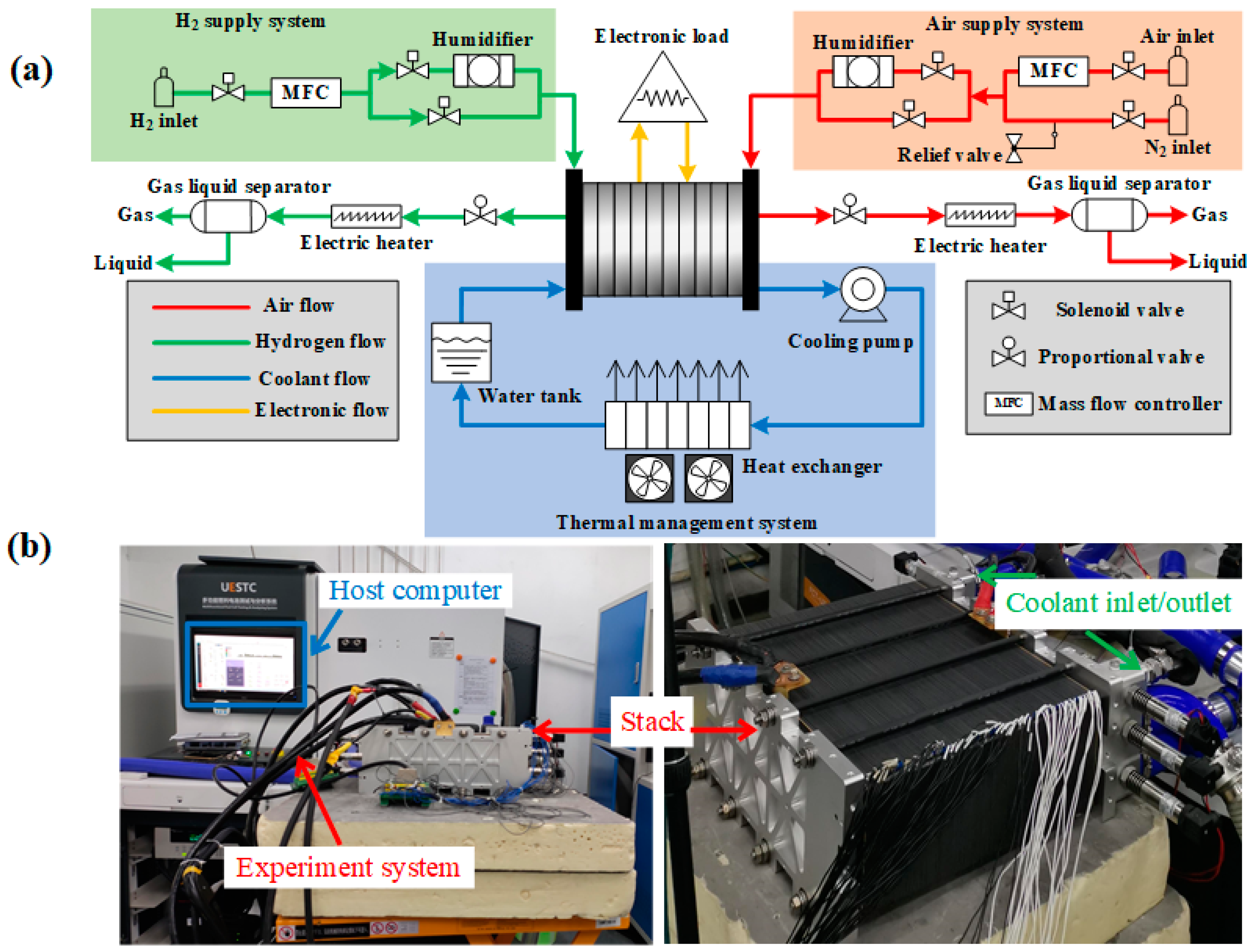
2. Experiment

The fuel cell stack performance and temperature characterization experiments are conducted on a high-power laboratory test platform with a 140-cell stack. Figure 1a shows the schematic diagram of the test system, and Figure 1b presents the experiment setups. The test system comprises subsystems of gas supply, thermal management, exhaust gas collection, and signal acquisition. The gas supply system uses a mass flow controller to provide the stack of nitrogen, hydrogen, and air at the set flow rate. The thermal management system controls the stack temperature by heating and cooling the coolant. The exhaust gas collection system collects the exhaust gas and liquid water from the cathode and anode outlets. The signal acquisition system tests and records pressure, temperature, and 140-cell voltages with a sampling time of 1 s.

Table 1. Stack technical specifications.

Parameter	Value
Stack cell number	140
Material of bipolar plate	Graphite
Active area	406 cm2
Thickness of PEM	0.0018 cm

lists the stack’s technical specifications. In the stack performance experiment, its temperature is controlled at 65 °C, and it is autonomously humidified by a membrane humidifier to an internal humidity of 95%. The hydrogen stoichiometry ratio is 1.3 without humidification. The air stoichiometry ratio is 2 with cathode off-gas humidification. The stoichiometric ratio is the ratio of the amount of reactant supplied to the amount of reactant required for the electrochemical reaction. The stoichiometry ratio is kept constant throughout the experiment, and the current sampling points are set in the range of 0~520 A in steps of 20 A, with a 3 min dwell at each point. The signal acquisition system records the cell voltages and other information at a sampling rate of 1 Hz.

Table 2. Operating parameters of temperature characteristics experiment.

Parameter	Value
Load current	467 A-487 A-507 A
Coolant flow rate	90 L/Min
Relative humidity	95%
Cathode inlet pressure	40 kPa
Anode inlet pressure	50 kPa
Ambient temperature	20 °C
Target temperature	65 °C
Maximum temperature	68 °C

lists the parameters of the stack temperature characterization experiment. To analyze the heat production and stack temperature response time, the target temperature and maximum temperature of the coolant are set to 65 °C and 68 °C, respectively, and the stack operates at three steady-state currents of 467 A, 487 A, and 507 A. The ambient temperature is 20 °C in the lab. The temperature is controlled close to the target temperature through the radiator, and the coolant temperature changes are recorded. Thermographic images at the stages of start-up, 467 A, and 507 A are taken to visualize the temperature distribution on the stack surface. The stack surface is divided into 25 segments labeled A~Y from the inlet end to the outlet end.

3. Model Development

3.1. Model Structure

Figure 2 illustrates the control model structure. The dynamic mechanistic model includes the stack mechanistic model and the heat transfer model. Then, a control model for stack thermal management combining the dynamic mechanistic model and the PSO+ANN algorithm is designed after decoupling the two thermal management factors: the coolant inlet temperature and the coolant inlet/outlet temperature difference. The models are simulated and analyzed using Simulink [32].

3.2. Dynamic Mechanistic Model

Figure 3 outlines the dynamic mechanistic model, including the stack mechanistic model and heat transfer model. The stack mechanistic model includes modeling of electrochemical, cathode water flow, anode water flow, and membrane hydration. The heat transfer model comprises stack heat exchange, piping, and radiator. The dynamic mechanistic model is constructed based on mechanistic and empirical formulas. The model parameters are listed in

Table 3. List of parameters and symbols used in the model.

Parameter	Symbol	Parameter	Symbol
Operating temperature	$T_{st}$	Cell number	$n$
O2 inlet partial pressure	$p_{O_2,in}$	Water’s molar mass	$M_{H_{2}O}$
H2 inlet partial pressure	$p_{H_2,in}$	Cathode flow channel volume	$V_{ca}$
Load current	$I$	Vapor’s gas constant	$R_v$
Cathode inlet pressure	$p_{ca,in}$	PEM thickness	$t_m$

.

3.2.1. Stack Voltage Model

The stack voltage can be analytically expressed by Nernst voltage and three voltage losses: activation, ohmic, and concentration [33,34,35]. Since boundary conditions limit some mathematical formulas, empirical formulas are used instead. The operating voltage of a single fuel cell is expressed as

$$v_{fc}=E-{\nu }_{act}-{\nu }_{ohm}-{\nu }_{conc}$$

(1)

where $v_{fc}$ is the output voltage of a single cell, the total voltage of the stack is calculated by multiplying the cell number by the output voltages of single cells, $E$ is the Nernst voltage, ${\nu }_{act}$ is the activation polarization voltage, ${\nu }_{ohm}$ is the ohmic loss, and ${\nu }_{conc}$ is the concentration polarization loss.

Based on the heating value at standard conditions, the Nernst voltage is expressed as [33]

$$\begin{array}{l}E=1.229-0.85\times {10}^{-3}(T_{st}-298.15)\\ \hspace{1em} +4.3085\times {10}^{-5}{T}_{st}[\ln (p_{H_2,in})+\frac{1}{2}\ln (p_{O_2,in})]\end{array}$$

(2)

In this paper, the activation polarization voltage uses an empirical equation, expressed as [20]

$${\nu }_{act}={\nu }_o+{\nu }_a(1-e^{-c_{1}I})$$

(3)

$$c1=10$$

(4)

The empirical voltage parameters ${\nu }_a$ and ${\nu }_o$ are expressed using empirical fitting equations as follows:

$$\begin{array}{l}{\mathcal{V}}_0=0.279-8.5\times {10}^{-4}(T_{st}-298.15)+4.308\times {10}^{-5}{T}_{st}[\ln (\frac{p_{ca,in}-p_{sat}}{1.01325})\\ \hspace{1em}\hspace{1em}+\frac{1}{2}\ln (\frac{0.1173(p_{ca,in}-p_{sat})}{1.01325})]\end{array}$$

(5)

$$\begin{array}{l}{\mathcal{V}}_a=(-1.618\times {10}^{-5}{T}_{st}+1.618\times {10}^{-2}){(\frac{p_{O_2,in}}{0.1173}+p_{sat})}^2+(1.8\times {10}^{-4}{T}_{st}\\ \hspace{1em}\hspace{1em}-0.166)(\frac{p_{O_2,in}}{0.1173}+p_{{}_{sat}})+(-5.8\times {10}^{-4}{T}_{{}_{st}}+0.5736)\end{array}$$

(6)

$$\begin{array}{l}{p}_{sat}=(2.6032\times {10}^{-6}{T}_{st}{}^5+3.1485\times {10}^{-4}{T}_{st}{}^4+2.3365\times {10}^{-2}{T}_{st}{}^3\\ \hspace{1em}\hspace{1em}+1.55\times T_{st}{}^2+42.8T_{st}+615.62)/1000\end{array}$$

(7)

where $p_{sat}$ is the saturated vapor pressure.

The ohmic loss is the voltage loss due to the membrane impedance and is calculated from Ohm’s law:

$${\nu }_{ohm}=I\cdot R_{ohm}$$

(8)

Membrane impedance is expressed as a function of membrane conductivity ${\sigma }_m$ and membrane thickness [36]:

$$R_{ohm}=\frac{t_m}{{\sigma }_m}$$

(9)

The membrane conductivity ${\sigma }_m$ is correlated with water content ${\lambda }_m$ and stack temperature $T_{fc}$, varying between 0 and 14 according to relative humidity [37], expressed as

$${\sigma }_m=b_1\exp (b_2(\frac{1}{303}-\frac{1}{T_{st}}))$$

(10)

$$b_1=(0.005139{\lambda }_m-0.00326)$$

(11)

$$b_2=350$$

(12)

The concentration voltage loss is caused by a drop in the reactant gas concentration, responsible for the rapid drop in the output voltage at high current density. The concentration voltage loss ${\nu }_{conc}$ is expressed as

$${\nu }_{conc}=I\cdot {(c_2\cdot \frac{I}{I_{\max }})}^{c_3}$$

(13)

$$I_{\max }=2.2$$

(14)

$$c_2=\{\begin{array}{cc}\begin{array}{c}(7.16\times {10}^{-4}{T}_{st}-0.622)(\frac{p_{O_2,in}}{0.1173}+p_{sat})\\ \hspace{1em}+(-1.45\times {10}^{-3}{T}_{st}+1.68)\end{array}& (\frac{p_{O_2,in}}{0.1173}+p_{sat})<2\\ \begin{array}{c}(8.66\times {10}^{-5}{T}_{st}-0.068)(\frac{p_{O_2,in}}{0.1173}+p_{sat})\\ \hspace{1em}+(-1.6\times {10}^{-4}{T}_{st}+0.54)\end{array}& (\frac{p_{O_2,in}}{0.1173}+p_{sat})>2\end{array}$$

(15)

$$c_3=2$$

(16)

where $I_{\max }$ [A/cm²] is the current density threshold that causes the output voltage to drop rapidly with the increase in current density. Its value is set using experiment results. $c_2$ is set using parametric nonlinear fitting, and $c_3$ is an empirical parameter [19].

3.2.2. Water Flow in the Cathode and Anode

The water flow model is used to describe the water mass inside the flow channel quantitatively and ultimately to obtain the dynamic characteristic of the relative humidity and the gas partial pressure. To simplify the calculations, some assumptions are made:

(1)

Gas behaves as an ideal gas and conforms to the ideal gas law.

(2)

The gas temperature inside the flow channel equals the stack temperature.

(3)

The temperature, pressure, and humidity inside the flow channel and at the exit are equal.

(4)

When the relative humidity of the gas is above 100%, the vapor condenses to liquid form but does not leave the stack. The liquid water evaporates into the gas or accumulates in the flow channel.

(5)

The flow channel volume is constant.

According to the mass conservation law, the following expression is valid for the water mass in the cathode flow channel [38]:

$$\frac{d{m}_{w,ca}}{dt}=W_{v,ca,in}-W_{v,ca,out}-W_{l,ca,out}+W_{w,m}+n\frac{I{M}_{H_{2}O}}{4F}$$

(17)

where the water mass passing through the membrane $W_{w,m}$ (kg/s) is derived from the membrane hydration model. $W_{v,ca,in}$ is the water mass entering the cathode, $W_{v,ca,out}$ is the water mass leaving the cathode, and $F$ is the Faraday constant. The maximum vapor mass $m_{v,\max ,ca}$ (kg/s) that can be accommodated on the cathode side is determined from the saturated vapor pressure:

$$m_{v,\max ,ca}=\frac{p_{sat}{V}_{ca}}{R_{\nu }{T}_{st}}$$

(18)

When liquid water is generated in the cathode, the vapor mass is maintained at the maximum vapor mass $m_{\nu ,\max ,ca}$ (kg). Further, the cathode relative humidity ${\varphi }_{ca}$ is expressed as

$${\varphi }_{ca}=\frac{p_{v,ca}}{p_{sat}(T_{st})}$$

(19)

where vapor partial pressure $p_{v,ca}$ (bar) is given by the ideal gas law:

$$p_{v,ca}=\frac{m_{v,ca}{R}_v{T}_{st}}{V_{ca}}$$

(20)

The cathode inlet gas consists of compressed air and gaseous water from the humidified water tank, and the cathode inlet air partial pressure $p_{a,ca,in}$ (bar) is given by the ideal gas law:

$$p_{\nu ,ca,in}={\varphi }_{ca,in}{p}_{sat}(T_{ca,in})$$

(21)

$$p_{a,ca,in}=p_{ca,in}-p_{\nu ,ca,in}$$

(22)

where $T_{ca,in}$ is the cathode inlet temperature and $p_{\nu ,ca,in}$ is the cathode inlet vapor partial pressure.

The relative humidity and inlet hydrogen partial pressure on the anode side are calculated similarly to the cathode side, and the following relationship exists for the water mass in the anode flow channel:

$$\frac{d{m}_{w,an}}{dt}=W_{v,an,in}-W_{v,an,out}-W_{l,an,out}-W_{v,m}$$

(23)

where $W_{v,an,in}$ is the water mass entering the anode and $W_{v,an,out}$ is the water mass leaving the anode.

3.2.3. Membrane Hydration

The water content and mass flow rate of water through the membrane are crucial factors in the operation. Water transport within the membrane is affected by two conditions: electro-osmotic resistance due to proton transfer from the anode to the cathode and back diffusion due to the water concentration gradient [39]. To simplify the calculations, some assumptions are made:

(1)

The water mass flow is distributed uniformly across the membrane.

(2)

The membrane water content is the average of the cathode water content ${\lambda }_{ca}$ and anode water content ${\lambda }_{an}$, ${\lambda }_{ca}$, and ${\lambda }_{an}$ can be expressed as

$${\lambda }_i=\{\begin{array}{cc}0.043+17.81{\varphi }_i-39.85{\varphi }_i^2+36{\varphi }_i^3& 0<{\varphi }_i\le 1\\ 14+1.4({\varphi }_i-1)& 1<{\varphi }_i\le 3\end{array}$$

(24)

where i represents the cathode and anode.

The electro-osmotic drag coefficient $n_d$ and water diffusion coefficient $D_w$ are determined by the water content of the membrane, and $D_w$ is also affected by the temperature [40]:

$$n_d=0.0029{\lambda }_m{}^2+0.05{\lambda }_m-3.4\times {10}^{-19}$$

(25)

$$D_{\lambda }=\{\begin{array}{cc}{10}^{-6}& {\lambda }_m<2\\ {10}^{-6}(1+2({\lambda }_m-2))& 2\le {\lambda }_m<3\\ {10}^{-6}(3-1.67({\lambda }_m-3))& 3\le {\lambda }_m<4.5\\ 1.25\times {10}^{-6}& {\lambda }_m\ge 4.5\end{array}$$

(26)

$$D_w=D_{\lambda }\exp (2416(\frac{1}{303}-\frac{1}{T_{st}}))$$

(27)

The water flow rate $N_{\nu ,m}$ depends on the two conditions of water transport as mentioned above:

$$N_{v,m}=n_d\frac{I}{F}-D_w\frac{(c_{v,ca}-c_{v,an})}{t_m}$$

(28)

where the first term is related to the electro-osmotic resistance, and the latter is related to the water concentration on the two sides of the membrane and the membrane’s diffusion coefficient. The water concentration on the two sides of the membrane $c_{v,ca}$ and $c_{v,an}$ are determined using the following equation:

$$c_{v,i}=\frac{{\rho }_{m,dry}\cdot {\lambda }_i}{M_{m,dry}}$$

(29)

where ${\rho }_{m,dry}$ is the density of the dry membrane (kg/cm³) and $M_{m,dry}$ is the molar mass of the dry membrane (kg/mol).

3.2.4. Stack Heat Exchange

The heat transfer model development can be divided into the modeling of the stack heat exchange, the radiator, and the piping. Ignoring the heat carried away by the reacting gases, the heat balance inside the stack is expressed as [41]

$$c_{st}{m}_{st}\frac{d{T}_{st}}{dt}=\frac{(v_0-v_f)\cdot I\cdot n}{1000}-c_d{M}_{cl}(T_{cl,out}-T_{cl,in})-Q_{atm}$$

(30)

where $c_{st}$ is the specific heat capacity of the stack (J/(kg·K)) and $m_{st}$ is the stack mass (kg). The first term on the right side is the heat generated by the stack, which is related to the output voltage and current obtained from the data manual of the stack. $v_0$ is related to the state of the water generated by the electrochemical reaction, and the value is set to 1.254~1.482 based on the water state as it leaves the stack. The second term is the heat absorbed by the coolant flowing through the stack. The third term is the thermal radiation resulting from the heat exchange between the stack and the environment.

3.2.5. Radiator

The cooling power of the plate-fin radiator is [42]

$$Q_{rad}=K\cdot S_a\cdot \Delta T_{rad}$$

(31)

where $K$ is the heat transfer coefficient of the radiator and is a function of coolant-side surface area, coolant flow rate, and radiator structure. $S_a$ is air-side surface area (m²) and $\Delta T_{rad}$ is the average temperature difference between the radiator and the environment.

3.2.6. Piping

The coolant piping is essentially a heat capacity model, and the volume of coolant is much larger than that of the electric stack or radiator, so there is a filtering effect on the temperature fluctuation of the coolant in the piping, denoted as [20]

$${\dot{T}}_{cl,p}=\frac{W_{cl}}{m_{pipe}}(T_{cl,p,in}-T_{cl,p})$$

(32)

where $T_{cl,p,in}$ is the piping inlet temperature (K), $T_{cl,p}$ is the piping temperature (K), $W_{cl}$ is the coolant flow rate (L/s), and $m_{pipe}$ is the coolant mass in the piping.

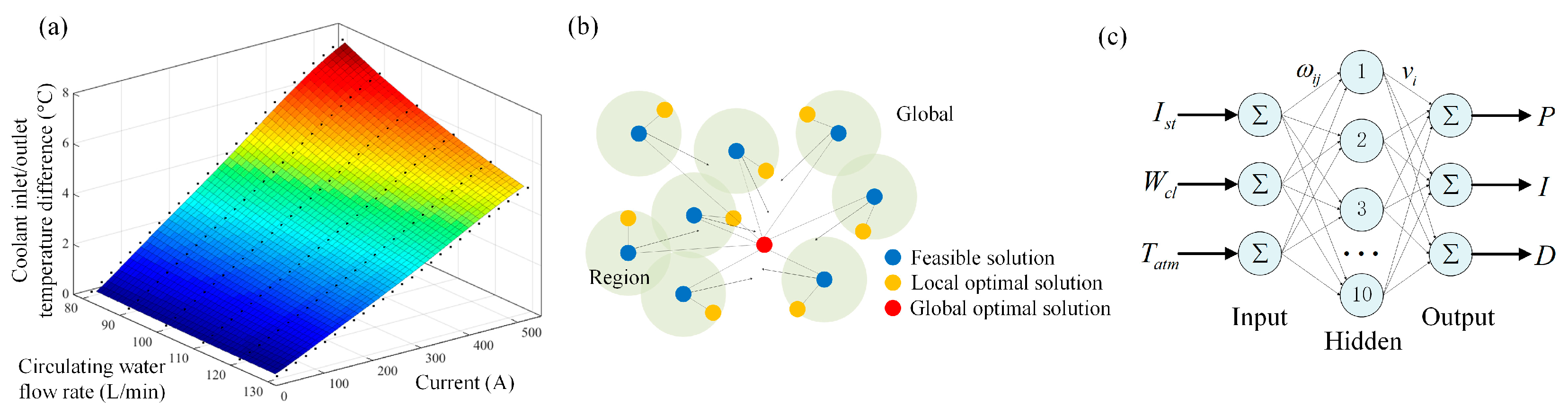
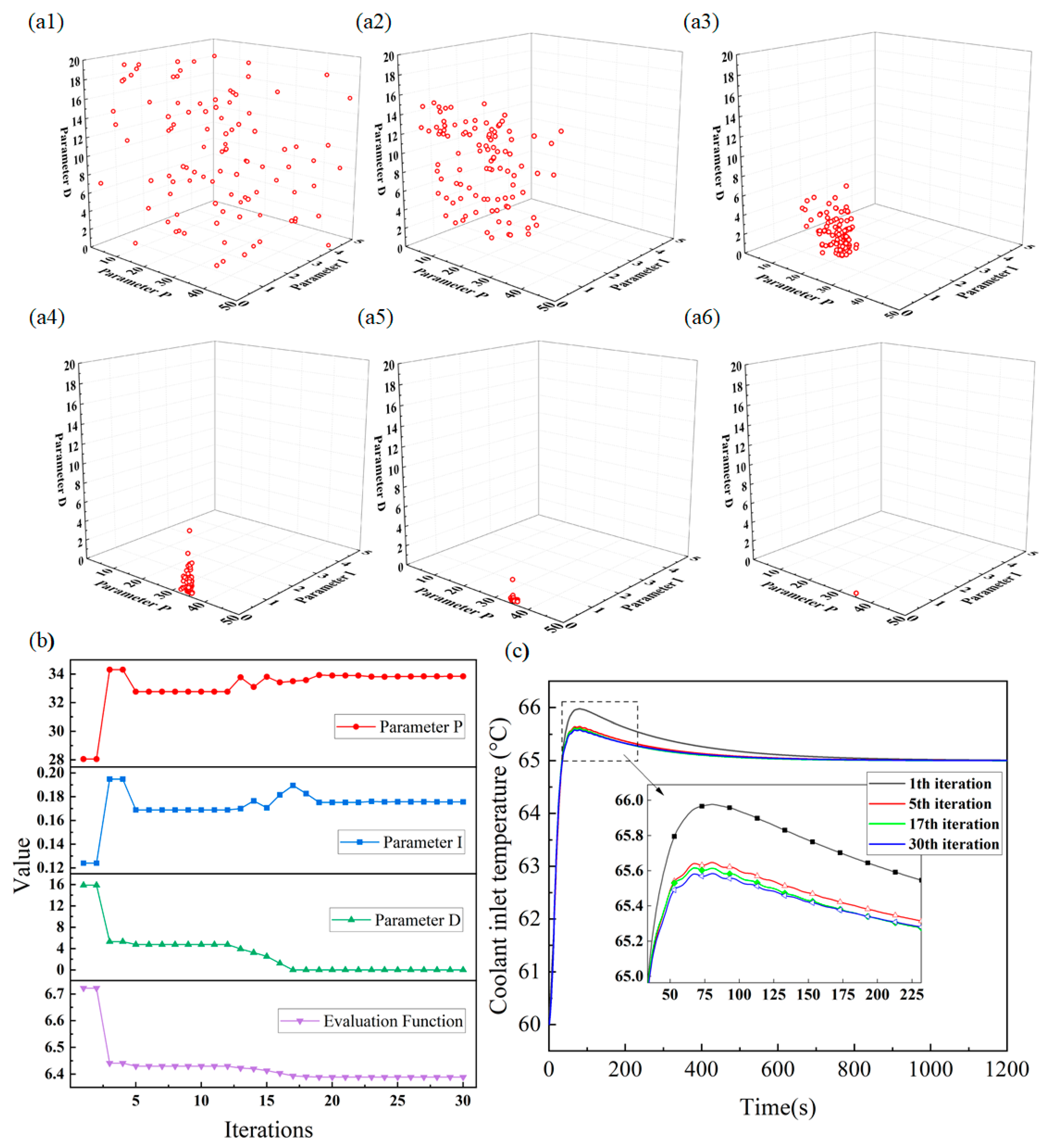
3.3. Control Model

The control model for the thermal management system proposed in this work includes two control parameters: coolant inlet/outlet temperature difference and coolant inlet temperature. This is because fuel cell system temperature control involves two aspects. One is that the radiator must provide sufficient power to timeously dissipate the heat absorbed by the coolant flowing through the stack. This prevents the heat from accumulating inside the stack, leading to high stack temperature and irreversible impact on the stack service life. The other aspect is that by precisely adjusting the coolant flow with the water pump, the coolant inlet/outlet temperature difference is controlled within a specific range, avoiding localized overheating or local condensation. It should be noted that the two aspects are correlated, thus prolonging the adjustment time of the thermal management system and causing temporary high stack temperatures, which is not conducive to its long-term operation.

To effectively control the two parameters, the coolant inlet/outlet temperature difference and coolant inlet temperature were first decoupled. The temperature difference is mainly related to the stack-generated heat and the coolant flow rate $W_{cl}$, while the stack-generated heat primarily depends on the current $I$. Thus the temperature difference can be expressed as

$$\Delta T_{st}=f(I,W_{cl})$$

(33)

Using the dynamic mechanistic model developed above, we carried out simulations to obtain the mapping for setting the coolant flow rates according to the currents, as shown in Figure 4a.

Table 4. Simulation parameters for coolant inlet/outlet temperature difference control.

Parameter	Symbol	Step	Interval
Load current	$I$	20 A	0~550 A
Coolant flow rate	$W_{cl}$	10 L/Min	80~130 SLPM

presents the simulation parameters. Then, we performed feedforward control on the coolant inlet/outlet temperature difference, achieving decoupling from the coolant inlet temperature.

The traditional proportional integral derivative (PID) control algorithm is often used to control coolant inlet temperature. However, the optimal PID parameters are not always available when the system is under different load currents and preset stack temperatures [43]. When the operating parameters are changed, the optimal values vary, and the control effect will be affected. To solve this issue, a control model combining the dynamic mechanistic model, PSO algorithm, and ANN model is developed in this paper to improve the coolant inlet temperature control.

Figure 4b shows the particle swarm optimization algorithm used in the control model. The PSO algorithm can find the optimal solution in an initial random particle group through several iterations. During the iterations, the particles update their current solutions by comparing the fitness value $f$, finally obtaining the optimal solution. The fitness value $f$ is based on the control effect (regulating time $t_s$, overshoots $\sigma$, and steady-state error $err$). The smaller the value of the fitness function, the better the control effect.

$$f=\log (t_s+1)+\log (\frac{2\cdot \sigma }{{10}^{-3}}+1)+\log (\frac{err}{{10}^{-2}}+1)$$

(34)

In total, 100 sets of PID parameters are selected under different coolant flow rates, operating temperatures, and load currents. The PSO algorithm is used to iterate each set of parameters for 30 iterations to obtain the optimal PID parameters for each operating condition.

The ANN model is one of the most popular data processing tools inspired by the biological structure of the brain and neurons. The trained ANN model can learn the relationship between input/output data and predict the output information based on the input data. In this work, the inputs for ANN training are the current, ambient temperature, and coolant flow rate. The outputs are the three PID parameters. The ANN model structure is shown in Figure 4c. The ANN model is trained with 70% of the parameter set as the training set, 15% as the test set, and 15% as the validation set. The ANN training process uses forward transmission and backpropagation to minimize the mean square error between the actual output value and the expected output value. The trained ANN is then applied to control the thermal management system. The results show that the model can predict the optimal PID parameters according to the current operating condition through the trained ANN, realizing the accurate control of the coolant inlet temperature under different load currents and preset stack temperatures.

4. Results and Discussion

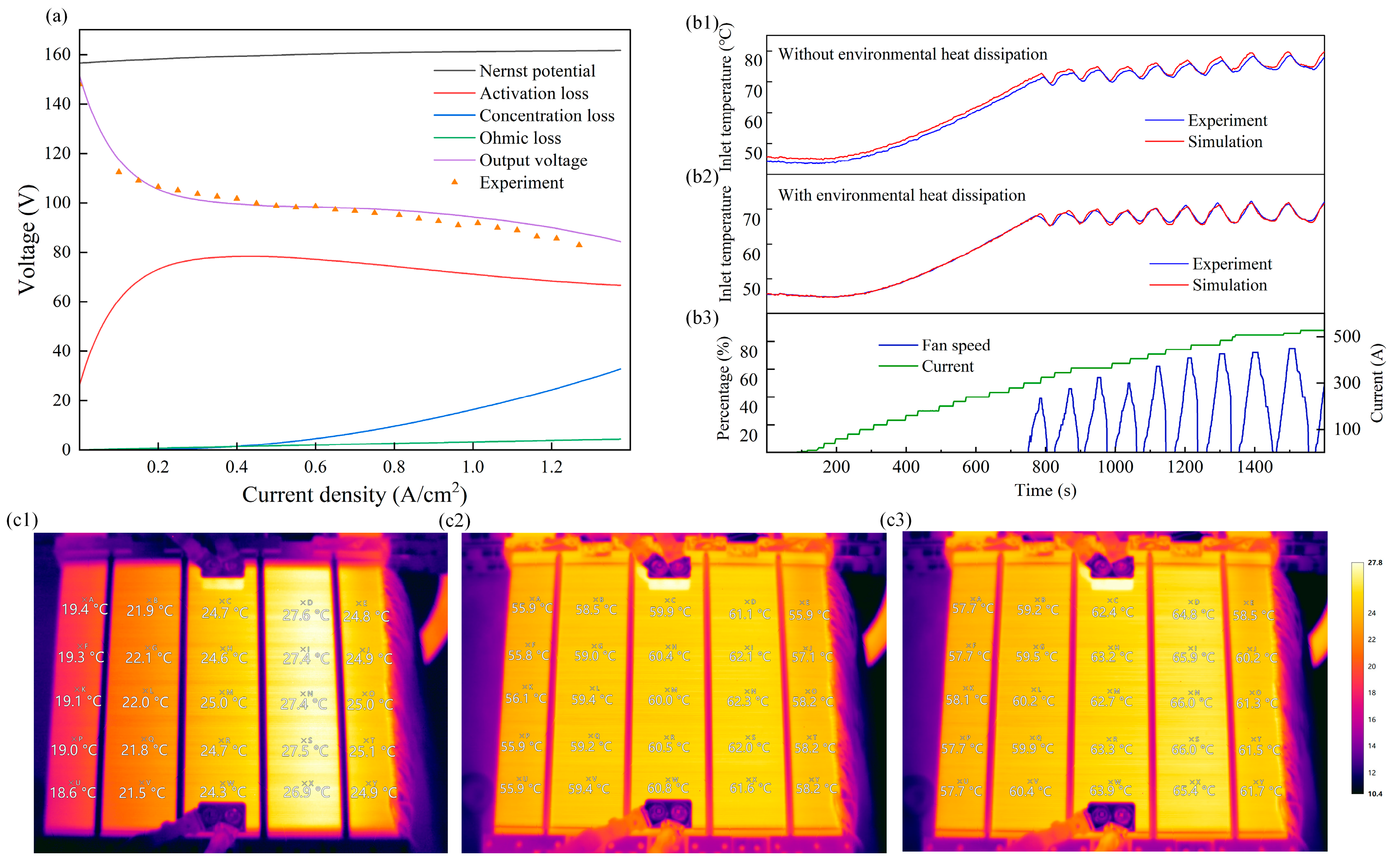
4.1. Model Validation

Figure 5a,b present the validation results of the dynamic mechanistic model developed in the previous section by comparing the simulation results with the experimental data. The thermal effects on the stack performance are also analyzed using the simulation results. The hydrogen/air stoichiometric ratio is set to 1.3/2, and the operating temperature is 65 °C. As elaborated in the modeling section, the system voltage decay is mainly caused by the Nernst voltage and three voltage losses (activation, ohmic, concentration). The stack performance experiment verifies the trends of their fluctuations with the current density. The average error between simulation and experiment is 0.79%, and the maximum error is 1.65%. The polarization curves of the simulation coincide with the experiment in Figure 5a. It can be concluded that the stack’s performance is in good agreement with the experimental results.

Figure 5c shows the thermographic images acquired during the temperature characterization experiment. In Figure 5(c1), in the startup stage, the temperature distribution inside the stack shows an increasing trend along the lateral direction while slightly decreasing on the rightmost side, and the higher temperature segments in the stack are concentrated in the middle, away from the coolant inlet. A possible reason for this phenomenon is that the segments near the coolant outlet have more heat exchange with the environment [13]. In addition, the electrochemical reaction generates a large amount of heat, which causes the coolant temperature to rise continuously after entering the stack, resulting in the stack temperature near the coolant outlet being significantly higher than that near the inlet. The maximum temperature difference reaches 9 °C. In Figure 5(c2,c3), when the current rises to 467 A and 507 A, the temperature increases with the rise in the current, and the temperature distribution characteristics are similar to those of the temperature distribution during the startup stage.

The simulation results of the heat transfer model are plotted in Figure 5b. At the beginning of the simulation, the coolant inlet temperature is set to 45 °C, and the target temperature is 65 °C, the same as the experiment. For the simulation with Simulink, shown in (b3), the experimentally obtained cooling fan operating data are used as the control condition for the radiator. In (b1), starting from the 750th second, the radiator controls the temperature near 65 °C through frequent start and stop. The temperature (~65 °C) is controlled, referring to the coolant temperature but with a deviation of about 1.5~2 °C caused by the heat dissipation. Since the temperature distribution on the stack surface usually varies, referring to the temperature distribution results from the experiments, a two-dimensional heat dissipation distribution of the 25 segments (except the surfaces of the end plates) is established in the model, denoted as

$$Q_{atm}={{\displaystyle \sum }}_{i=1}^5{{\displaystyle \sum }}_{j=1}^{5}h\cdot S_{ij}(T_{ij,st}-T_{atm})$$

(35)

where $h$ is the environmental heat dissipation coefficient and $S_{ij}$ and $T_{ij,st}$ are the area (m²) and average temperature (K) of the segment in row $i$, column $j$. In (b2), the simulation is consistent with the experimental results after adding the heat dissipation, proving that the heat dissipation leads to bias for the stack thermal effect.

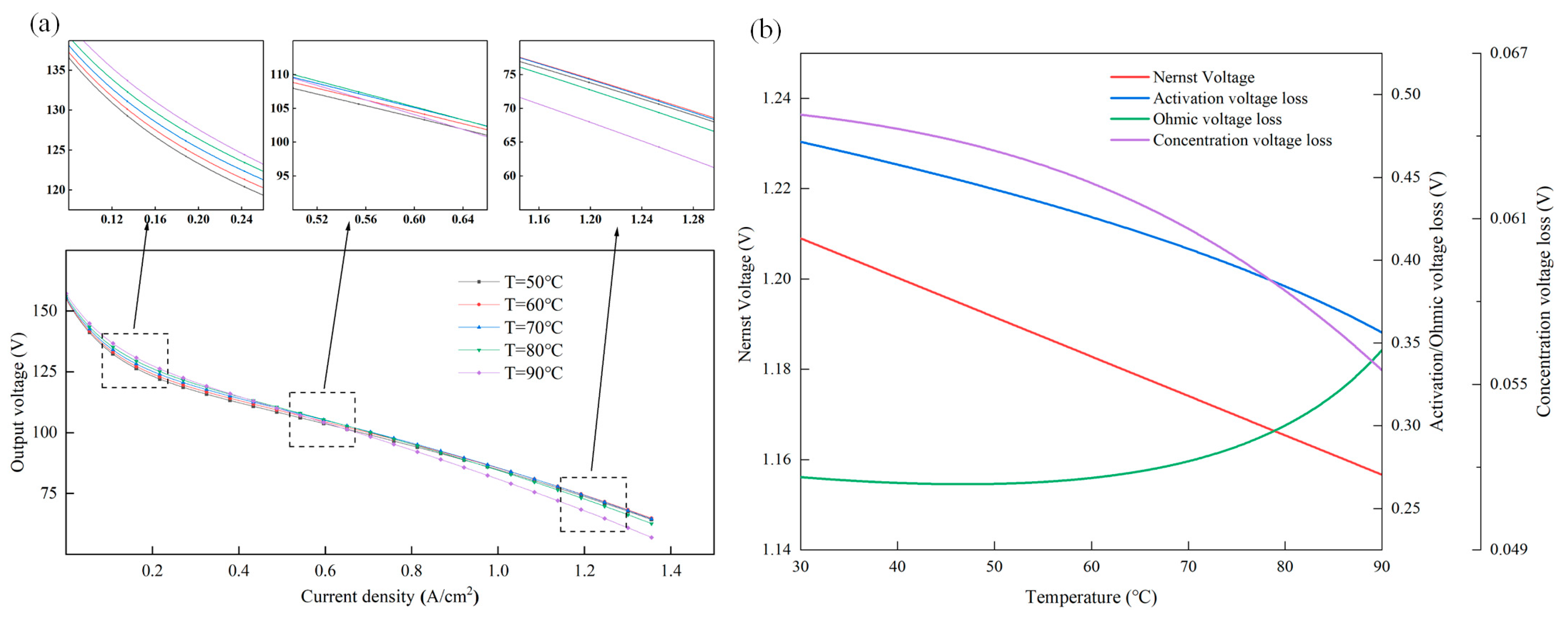
4.2. Parametric Effect Analysis of Temperature

Figure 6a shows the polarization curves at different temperatures obtained from the dynamic mechanistic model in the previous section. At an operating current density of 0.2 A/cm², activation loss is the major part of the voltage loss, and the output voltage increases with temperature. This is because the increase in catalyst activity and the acceleration of the electrochemical reaction rate lead to a decrease in the activation loss. When the stack is operated at a current density of 0.6 A/cm², the activation loss ceases to increase, and the linear increase in ohmic loss with current density makes it a major part of the voltage loss. Excessive temperatures (90 °C) cause the output voltage to drop. At an operating current density of 1.2 A/cm², the output voltage at 90 °C is significantly lower than at other temperatures due to a significant increase in the ohmic loss and concentration loss. The reason is that the excessively high operating temperature vaporizes the water in the MEA, the water content of the membrane decreases, and then the proton transport capacity decreases.

The variation in voltage losses at different temperatures is shown in Figure 6b. The activation loss decreases with increasing temperature, and it is more evident at high current density than at low current density because a suitable temperature promotes the electrochemical reaction in the stack. The temperature increase accelerates the reaction rate, leading to a decrease in the activation loss. The ohmic loss increases dramatically at high temperatures due to the decrease in the water content of the proton exchange membrane caused by high temperatures. Temperature increase leads to a slight reduction in the concentration loss at high current densities.

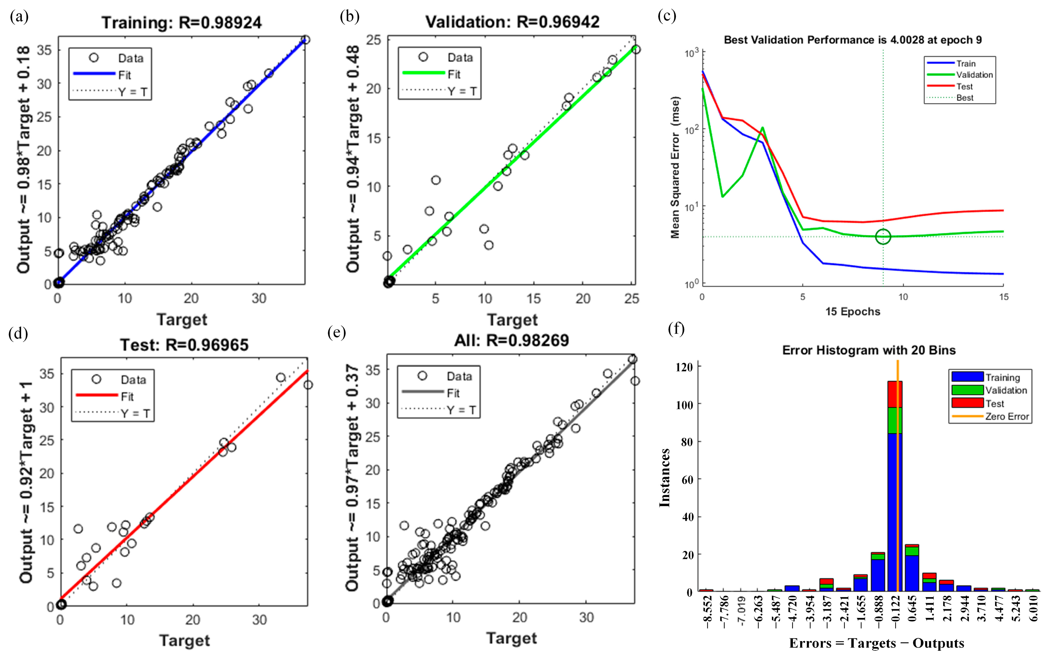
4.3. Training Results

Figure 7 shows the convergence of the particle swarm optimization algorithm for a current of 500 A, coolant flow rate of 100 L/min, and ambient temperature of 25 °C. In Figure 7(a1), the initialized particles are equally distributed in the three-dimensional space. In Figure 7(a2–a6), the particles gradually converge in the iterative process and converge to the optimal solution in the 18th iteration, which is taken as the optimal control parameter for this working condition. In Figure 7b, the PID parameters converge to near the optimal value in the fifth iteration, corresponding to Figure 7(a4), in which the particle swarm is clustered near the optimal position. The algorithm reaches the optimal solution in the 18th iteration, and the fitness values are no longer reduced. In Figure 7c, the overshoot and regulation time of the temperature response are minimized after the 17th iteration, and the control effect reaches the optimum. The control parameter values are P = 33.84, I = 0.176, and D = 0.

In Figure 8, the validation results of the neural network model trained using the PSO algorithm are shown to evaluate the model’s performance in terms of MSE, error distribution histogram, and R² for different types of samples. In Figure 8a,b,d,e, the model demonstrates good results, with R² from each sample being greater than 0.969. The MSE is shown in Figure 8c, where the MSE decreases with iterations and reaches a minimum at the ninth iteration.

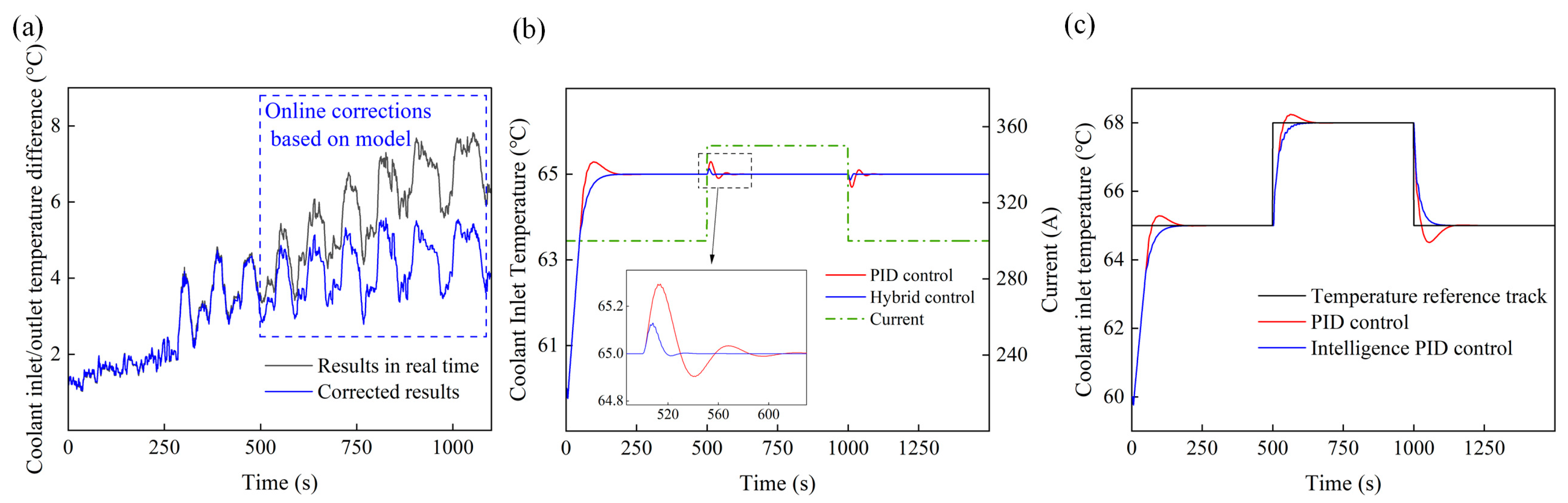
4.4. Control Model Effectiveness

Figure 9a compares the simulation and experimental results of coolant inlet and outlet temperature difference feedforward control. In the loading experiment, during the period 0~300 s, the stack operates in the low-current range with low heat generation, and the coolant inlet and outlet temperature difference is within 2 °C. During the period 300~500 s, the operating current gradually increases, the heat generation inside the stack increases, and the temperature difference reaches 5 °C. After 500 s, the temperature difference reaches 8 °C when the stack is loaded to a higher current, and the temperature difference is 5.8 °C on average. After applying the feedforward correction, although the temperature fluctuation makes the temperature difference slightly higher than 5 °C at some moments, the coolant inlet and outlet temperature difference is always kept within 5 °C, with an average temperature difference of 4.3 °C. Therefore, the model effectively fulfills the operational requirement.

In Figure 9b,c, the dynamic performance of the control model is simulated. In Figure 9b, the initial temperature of the stack is set to 60 °C, the target temperature is 65 °C, and the current is 300 A. At this time, the stack is in the heating stage, and the overshoot reaches 5.72% compared to that under traditional PID control. Applying the control model, no overshoot is found, and the temperature stabilizes at the set temperature much faster. After reaching the target temperature, the stack is in the heat dissipation stage, and a current loading in the 500th second and a load shedding in the 1000th second are set to test the dynamic performance. The temperature overshoot under the traditional PID control reaches 5.00%, the regulation time is 115 s, and many fluctuations in the temperature response curve indicate poor dynamic performance. The temperature can be stabilized at the set temperature quickly under the control model; the regulation time is only 30 s, and the overshoot is 2.60%. Accordingly, when the temperature rises and the load changes, the performance of the control model is significantly improved compared with the traditional PID control. It can be concluded that the control model has outstanding anti-disturbance and control capabilities for the load current changes in the experiment.

The control model also has a reliable control effect on the perturbation from the set temperature changes. Dynamic simulation experiments are designed for the model, with the initial stack temperature of 60 °C, the target temperature of 65 °C, and the current of 300 A. After the operation is stabilized, the target temperature is increased to 68 °C in the 500th second and decreased back to 65 °C in 1000th second. The control effect is shown in Figure 9c. Respectively, 8% and 16.60% overshoots of the traditional PID control occur during the temperature increase and decrease. The response curve with the control model changes smoothly during two dynamic changes without overshoot, and the regulation time is shorter.

5. Conclusions

In this study, an effective control model is developed for the stack thermal management system to solve the issues of unsatisfactory thermal control accuracy and response speed under complex operating conditions with constantly changing load current and preset stack temperature.

First, a dynamic mechanistic model of the fuel cell stack and thermal management system was created. It was then verified by comparing the simulation and experimental results, with a stack performance error of no more than 1.65% and a temperature error of no more than 0.90%. Then, we designed the mapping for setting the coolant flow rates according to the currents to control the coolant inlet/outlet temperature difference and decoupled the two parameters (coolant inlet/outlet temperature difference and coolant inlet temperature). The simulation results showed that the coolant inlet/outlet temperature difference was always within 5 °C, with an average temperature difference of 4.3 °C. Finally, a control model was developed based on the fuel cell’s dynamic mechanistic model and PSO+ANN algorithm. The ANN showed excellent training results, and the R² from each sample was greater than 0.969. It was applied to compare with the traditional PID algorithm, and we found that the regulation time of coolant inlet temperature as the current changed was reduced by more than 74%, and the overshoot was reduced by more than 50%. Therefore, we can conclude that the control model can control the temperature better than the traditional PID algorithm.

We focused on one-dimensional control modeling in this study. In future work, the model can be extended to multi-dimensional to gain more accurate and comprehensive temperature distribution information inside the stack, further improving the thermal management effectiveness.

References

- Wang, Y.; Ruiz Diaz, D.F.; Chen, K.S.; Wang, Z.; Adroher, X.C. Materials, Technological Status, and Fundamentals of PEM Fuel Cells—A Review. Mater. Today 2020, 32, 178–203. [Google Scholar] [CrossRef]
- Song, Y.; Zhang, C.; Ling, C.-Y.; Han, M.; Yong, R.-Y.; Sun, D.; Chen, J. Review on Current Research of Materials, Fabrication and Application for Bipolar Plate in Proton Exchange Membrane Fuel Cell. Int. J. Hydrogen Energy 2020, 45, 29832–29847. [Google Scholar] [CrossRef]
- Wang, G.; Yu, Y.; Liu, H.; Gong, C.; Wen, S.; Wang, X.; Tu, Z. Progress on Design and Development of Polymer Electrolyte Membrane Fuel Cell Systems for Vehicle Applications: A Review. Fuel Process. Technol. 2018, 179, 203–228. [Google Scholar] [CrossRef]
- Ahmad, S.; Nawaz, T.; Ali, A.; Orhan, M.F.; Samreen, A.; Kannan, A.M. An Overview of Proton Exchange Membranes for Fuel Cells: Materials and Manufacturing. Int. J. Hydrogen Energy 2022, 47, 19086–19131. [Google Scholar] [CrossRef]
- Yang, B.; Li, J.; Li, Y.; Guo, Z.; Zeng, K.; Shu, H.; Cao, P.; Ren, Y. A Critical Survey of Proton Exchange Membrane Fuel Cell System Control: Summaries, Advances, and Perspectives. Int. J. Hydrogen Energy 2022, 47, 9986–10020. [Google Scholar] [CrossRef]
- Schmittinger, W.; Vahidi, A. A Review of the Main Parameters Influencing Long-Term Performance and Durability of PEM Fuel Cells. J. Power Sources 2008, 180, 1–14. [Google Scholar] [CrossRef]
- Yan, W.-M.; Chen, F.; Wu, H.-Y.; Soong, C.-Y.; Chu, H.-S. Analysis of Thermal and Water Management with Temperature-Dependent Diffusion Effects in Membrane of Proton Exchange Membrane Fuel Cells. J. Power Sources 2004, 129, 127–137. [Google Scholar] [CrossRef]
- Li, Q.; Liu, Z.; Sun, Y.; Yang, S.; Deng, C. A Review on Temperature Control of Proton Exchange Membrane Fuel Cells. Processes 2021, 9, 235. [Google Scholar] [CrossRef]
- Zhang, G.; Kandlikar, S.G. A Critical Review of Cooling Techniques in Proton Exchange Membrane Fuel Cell Stacks. Int. J. Hydrogen Energy 2012, 37, 2412–2429. [Google Scholar] [CrossRef]
- Fang, C.; Xu, L.; Cheng, S.; Li, J.; Jiang, H.; Ouyang, M. Sliding-Mode-Based Temperature Regulation of a Proton Exchange Membrane Fuel Cell Test Bench. Int. J. Hydrogen Energy 2017, 42, 11745–11757. [Google Scholar] [CrossRef]
- Zhang, G.; Jiao, K. Multi-Phase Models for Water and Thermal Management of Proton Exchange Membrane Fuel Cell: A Review. J. Power Sources 2018, 391, 120–133. [Google Scholar] [CrossRef]
- Yu, S.; Jung, D. Thermal Management Strategy for a Proton Exchange Membrane Fuel Cell System with a Large Active Cell Area. Renew. Energy 2008, 33, 2540–2548. [Google Scholar] [CrossRef]
- Zhang, Q.; Xu, L.; Li, J.; Ouyang, M. Performance Prediction of Proton Exchange Membrane Fuel Cell Engine Thermal Management System Using 1D and 3D Integrating Numerical Simulation. Int. J. Hydrogen Energy 2018, 43, 1736–1748. [Google Scholar] [CrossRef]
- Thomas, A.; Maranzana, G.; Didierjean, S.; Dillet, J.; Lottin, O. Measurements of Electrode Temperatures, Heat and Water Fluxes in PEMFCs: Conclusions about Transfer Mechanisms. J. Electrochem. Soc. 2013, 160, F191–F204. [Google Scholar] [CrossRef]
- Rahgoshay, S.M.; Ranjbar, A.A.; Ramiar, A.; Alizadeh, E. Thermal Investigation of a PEM Fuel Cell with Cooling Flow Field. Energy 2017, 134, 61–73. [Google Scholar] [CrossRef]
- Cao, T.-F.; Lin, H.; Chen, L.; He, Y.-L.; Tao, W.-Q. Numerical Investigation of the Coupled Water and Thermal Management in PEM Fuel Cell. Appl. Energy 2013, 112, 1115–1125. [Google Scholar] [CrossRef]
- Hosseinzadeh, E.; Rokni, M.; Rabbani, A.; Mortensen, H.H. Thermal and Water Management of Low Temperature Proton Exchange Membrane Fuel Cell in Fork-Lift Truck Power System. Appl. Energy 2013, 104, 434–444. [Google Scholar] [CrossRef]
- Nolan, J.; Kolodziej, J. Modeling of an Automotive Fuel Cell Thermal System. J. Power Sources 2010, 195, 4743–4752. [Google Scholar] [CrossRef]
- Zhao, X.; Li, Y.; Liu, Z.; Li, Q.; Chen, W. Thermal Management System Modeling of a Water-Cooled Proton Exchange Membrane Fuel Cell. Int. J. Hydrogen Energy 2015, 40, 3048–3056. [Google Scholar] [CrossRef]
- Liso, V.; Nielsen, M.P.; Kær, S.K.; Mortensen, H.H. Thermal Modeling and Temperature Control of a PEM Fuel Cell System for Forklift Applications. Int. J. Hydrogen Energy 2014, 39, 8410–8420. [Google Scholar] [CrossRef]
- Han, Z.; He, L.; Niu, Z.; Liu, Z. A Review and Prospect for Temperature Control Strategy of Water-Cooled PEMFC. In Proceedings of the 2017 36th Chinese Control Conference (CCC), Dalian, China, 26–28 July 2017; IEEE: Piscataway, NJ, USA, 2017; pp. 9062–9068. [Google Scholar]
- Cheng, S.; Fang, C.; Xu, L.; Li, J.; Ouyang, M. Model-Based Temperature Regulation of a PEM Fuel Cell System on a City Bus. Int. J. Hydrogen Energy 2015, 40, 13566–13575. [Google Scholar] [CrossRef]
- Saygili, Y.; Eroglu, I.; Kincal, S. Model Based Temperature Controller Development for Water Cooled PEM Fuel Cell Systems. Int. J. Hydrogen Energy 2015, 40, 615–622. [Google Scholar] [CrossRef]
- Chen, F.; Yu, Y.; Gao, Y. Temperature Control for Proton Exchange Membrane Fuel Cell Based on Current Constraint with Consideration of Limited Cooling Capacity. Fuel Cells 2017, 17, 662–670. [Google Scholar] [CrossRef]
- Lin, X.; Huang, J. Applications of Heuristic Dynamic Programming in the Proton Exchange Membrane Fuel Cell Temperature Control. In Proceedings of the 2012 Power Engineering and Automation Conference, Wuhan, China, 18–20 September 2012; IEEE: Piscataway, NJ, USA, 2012; pp. 1–4. [Google Scholar]
- Saadi, A.; Becherif, M.; Hissel, D.; Ramadan, H.S. Dynamic Modeling and Experimental Analysis of PEMFCs: A Comparative Study. Int. J. Hydrogen Energy 2017, 42, 1544–1557. [Google Scholar] [CrossRef]
- Cheng, S.-J.; Liu, J.-J. Nonlinear Modeling and Identification of Proton Exchange Membrane Fuel Cell (PEMFC). Int. J. Hydrogen Energy 2015, 40, 9452–9461. [Google Scholar] [CrossRef]
- Miao, J.-M.; Cheng, S.-J.; Wu, S.-J. Metamodel Based Design Optimization Approach in Promoting the Performance of Proton Exchange Membrane Fuel Cells. Int. J. Hydrogen Energy 2011, 36, 15283–15294. [Google Scholar] [CrossRef]
- Wilberforce, T.; Olabi, A.G. Proton Exchange Membrane Fuel Cell Performance Prediction Using Artificial Neural Network. Int. J. Hydrogen Energy 2021, 46, 6037–6050. [Google Scholar] [CrossRef]
- Han, I.-S.; Park, S.-K.; Chung, C.-B. Modeling and Operation Optimization of a Proton Exchange Membrane Fuel Cell System for Maximum Efficiency. Energy Convers. Manag. 2016, 113, 52–65. [Google Scholar] [CrossRef]
- Tian, P.; Liu, X.; Luo, K.; Li, H.; Wang, Y. Deep Learning from Three-Dimensional Multiphysics Simulation in Operational Optimization and Control of Polymer Electrolyte Membrane Fuel Cell for Maximum Power. Appl. Energy 2021, 288, 116632. [Google Scholar] [CrossRef]
- Spiegel, C. PEM Fuel Cell Modeling and Simulation Using Matlab; Academic Press: Amsterdam, The Netherlands; Elsevier: Boston, MA, USA, 2008; ISBN 978-0-12-374259-9. [Google Scholar]
- Amphlett, J.C.; Baumert, R.M.; Mann, R.F.; Peppley, B.A.; Roberge, P.R.; Harris, T.J. Performance Modeling of the Ballard Mark IV Solid Polymer Electrolyte Fuel Cell: I. Mechanistic Model Development. J. Electrochem. Soc. 1995, 142, 1. [Google Scholar] [CrossRef]
- Seyezhai, R.; Mathur, B.L. Mathematical Modeling of Proton Exchange Membrane Fuel Cell. Int. J. Comput. Appl. 2011, 20, 82–96. [Google Scholar] [CrossRef]
- Amphlett, J.C.; Baumert, R.M.; Mann, R.F.; Peppley, B.A.; Roberge, P.R.; Harris, T.J. Performance Modeling of the Ballard Mark IV Solid Polymer Electrolyte Fuel Cell: II. Empirical Model Development. J. Electrochem. Soc. 1995, 142, 9–15. [Google Scholar] [CrossRef]
- Kim, J.; Lee, S.; Srinivasan, S.; Chamberlin, C.E. Modeling of Proton Exchange Membrane Fuel Cell Performance with an Empirical Equation. J. Electrochem. Soc. 1995, 142, 2670–2674. [Google Scholar] [CrossRef]
- Springer, T.E.; Zawodzinski, T.A.; Gottesfeld, S. Polymer Electrolyte Fuel Cell Model. J. Electrochem. Soc. 1991, 138, 2334–2342. [Google Scholar] [CrossRef]
- Bao, C.; Ouyang, M.; Yi, B. Modeling and Control of Air Stream and Hydrogen Flow with Recirculation in a PEM Fuel Cell System—I. Control-Oriented Modeling. Int. J. Hydrogen Energy 2006, 31, 1879–1896. [Google Scholar] [CrossRef]
- Dutta, S.; Shimpalee, S.; Van Zee, J.W. Numerical Prediction of Mass-Exchange between Cathode and Anode Channels in a PEM Fuel Cell. Int. J. Heat Mass Transf. 2001, 44, 2029–2042. [Google Scholar] [CrossRef]
- Zawodzinski, T.A.; Derouin, C.; Radzinski, S.; Sherman, R.J.; Smith, V.T.; Springer, T.E.; Gottesfeld, S. Water Uptake by and Transport through Nafion® 117 Membranes. J. Electrochem. Soc. 1993, 140, 1041–1047. [Google Scholar] [CrossRef]
- Yu, X.; Zhou, B.; Sobiesiak, A. Water and Thermal Management for Ballard PEM Fuel Cell Stack. J. Power Sources 2005, 147, 184–195. [Google Scholar] [CrossRef]
- Hu, P.; Cao, G.-Y.; Zhu, X.-J.; Hu, M. Coolant Circuit Modeling and Temperature Fuzzy Control of Proton Exchange Membrane Fuel Cells. Int. J. Hydrogen Energy 2010, 35, 9110–9123. [Google Scholar] [CrossRef]
- Rabbani, A.; Rokni, M. Dynamic Characteristics of an Automotive Fuel Cell System for Transitory Load Changes. Sustain. Energy Technol. Assess. 2013, 1, 34–43. [Google Scholar] [CrossRef]