Abstract
Faulting refers to the common and significant distress in Jointed Plain Concrete Pavement (JPCP), which has an adverse impact on the pavement roughness. Nevertheless, the existing fault prediction models continue to heavily rely on conventional linear regression techniques or basic machine learning approaches, which leaves room for improvement in training efficiency and interpretability. To enhance training efficiency and accuracy, this study developed five novel faulting prediction models. These models are based on five basic machine learning algorithms: Random Forest (RF), Additive Boosting (AdaBoost), Gradient Boosting Decision Tree (GBDT), Light Gradient Boosting Machine (LightGBM), and Categorical Boost (CatBoost), combined with the tree-structured Parzen estimator (TPE). The five models are TPE-RF, TPE-AdaBoost, TPE-GBDT, TPE-LightGBM, and TPE-CatBoost. In addition to selecting the best-performing model, this study incorporated the Shapley Additive Explanation (SHAP) technique and developed TPE-SHAP-CatBoost to improve the interpretability of the model’s predictions. The process involved extracting historical data on pavement performance, including 17 variables, from the Long-Term Pavement Performance (LTPP) database for 160 instances of observation. Firstly, the Boruta method was used to identify the final set of input variables. Secondly, the TPE technique, which is a Bayesian optimization method, was applied to automatically select the optimal hyperparameters for the base models. Finally, SHAP was used to provide both global and local explanations of the model’s outputs. The results indicate that the TPE-CatBoost model achieves the highest accuracy with an R2 value of 0.906. Furthermore, the TPE-SHAP-CatBoost model identified the primary factors influencing faulting by incorporating SHAP and provided explanations of the model’s results at both the global and local levels. These research findings highlight the ability of the proposed model to accurately predict faulting, providing precise and interpretable guidance for pavement maintenance while reducing workload for pavement engineers in data collection and management.
1. Introduction
Transportation infrastructure projects have always been crucial assets for every country, playing a vital role in economic development and societal progress []. Pavements typically handle approximately 80% of passenger transportation tasks in various countries []. However, pavements can sustain damage to varying degrees during their service life due to factors such as traffic loads and environmental conditions. An annual expenditure of over USD 400 billion is allocated globally for pavement construction, maintenance, and repair (M&R) []. Rigid pavements are widely recognized for their durability, long lifespan, high resistance to heavy traffic, and adaptability to harsh weather conditions []. JPCP is the most common and extensively used type within rigid pavements []. However, with time, JPCP experiences various damages due to multiple influencing factors, such as faulting, pumping, and corner spalling. Among these factors, faulting is regarded as one of the most significant structural and functional failures in JPCP, which is characterized by height differences along transverse joints. Faulting on the pavement surface result in increased road roughness, leading to higher fuel consumption, more frequent traffic accidents, increased greenhouse gas emissions, and higher maintenance costs, all of which are inconsistent with environmental requirements []. Extensive research has been conducted to develop accurate predictive models for faulting characteristics, highlighting its importance in the field.
Historical prediction models for faulting have traditionally been categorized into two main types: regression-based models and machine-learning-based models. Initially, regression models were widespread. For instance, in 1994, Simpson et al. [] created two distinct models to predict faulting in JPCP. One model focused on the presence of dowel bars, while the other aimed to address their absence. However, the R-squared values for these two models were 0.534 and 0.550, respectively, which suggests a low level of accuracy in real-world scenarios. The models’ low accuracy can be attributed to the limited dataset size (less than one hundred) and the inability of a linear combination of input variables to capture the complex nonlinear relationships that influence pavement failures. Similarly, Yu et al. [] employed regression methods to develop a fault prediction model. To enhance the model’s performance, the dataset was expanded to include 146 samples, and additional variables such as modified drainage coefficient and average transverse joint spacing were introduced. The model achieved an R-squared value of 0.60, indicating moderate improvement. The AASHTO report (2010) utilized a methodology of progressively increasing failure rates over time to represent the average faulting. Additional variables, including weather information, deformation, and erodibility factor, were incorporated into the model. Despite the improvement in the model’s R-squared value to 0.71, it became excessively complex. Wei Ker et al. [] employed various contemporary regression techniques, such as the generalized linear model (GLM) and generalized additive model (GAM), to enhance the accuracy of the model’s predictions. Moreover, they identified variables with notable influences, such as pavement age, yearly ESALs, and so on, for the prediction of faulting. The model, developed utilizing 302 data points, achieved an R-squared value of 0.6039.
Researchers have adopted machine learning techniques to address the challenges associated with predicting faulting due to the limitations of regression-based methods. Saghafi et al. [] attempted to develop a faulting prediction model using Artificial Neural Networks (ANNs). The model used input variables such as pavement age, base type and material description, base thickness, erodibility, resilient modulus, etc. The model attained an R2 value of 0.94, indicating significantly higher accuracy compared to the linear-regression-based model with an R2 value of 0.51. This suggests that neural network algorithms, which can handle complex nonlinear relationships, are better suited for fault prediction than linear regression algorithms. Moreover, Wang and Tsai [] conducted a detailed study in which they developed four ANN models utilizing the ANN approach. They categorized the input variables into four groups: 4, 6, 8, and 10 variables. The ANN model, which consisted of eight variables, was ultimately recognized as the superior choice due to its low computation error and high computational speed. Nevertheless, the overall accuracy of the developed models in this study was not high, primarily attributed to the unreasonable settings of ANN hyperparameters and inappropriate feature selection. Hence, Ehsani et al. [] commenced their study by addressing the challenge of accurate feature selection in ANN prediction models. Their research involved initially developing a model that incorporated all input variables and subsequently applying the NSGA II-MLP algorithm to identify the essential variables. Two simplified models were constructed using ANN and RF, respectively. Through comparison and analysis, they identified the top-performing model, which achieved an R2 value of 0.92. In a similar vein, Ehsani et al. [] employed metaheuristic algorithms to select features and optimize ANN hyperparameters in another study. Following hyperparameter optimization, the best model attained an R2 value of 0. 976. Although ANN has demonstrated excellent accuracy, it still lacks interpretability. This is due to the fact that ANN is commonly regarded as a “black box” model, meaning it lacks the ability to explicitly explain the relationship between input variables and output results. In real-world applications, pavement management personnel aim to identify key variables that have a significant impact on pavement performance. This strategic knowledge not only enhances the reliability of the models, but also helps reduce data collection expenses.
Traditional methods in the field of feature selection primarily minimize the loss function by choosing a subset of features that are specific to the model. The Boruta algorithm serves a distinct purpose by identifying all feature subsets associated with the dependent variable []. Alongside, SHAP and TPE are powerful analysis tools. SHAP applies game theory to calculate the marginal contribution of each feature to the model’s output, assigning specific importance values to ensure both global and local interpretability []. As a result, SHAP has been widely applied in various domains. On the other hand, hyperparameter optimization involves finding the best combination of hyperparameters for a machine learning model. Setting hyperparameters is a complicated process that can significantly affect model performance. A Python library, TPE, employs a Bayesian optimization algorithm and surrogate targets to promptly and accurately determine the optimal hyperparameters, thus enhancing the model’s performance [,,,]. Combining the Boruta algorithm improves both the speed and quality of feature selection. Additionally, the addition of the TPE learning framework allows for automatic optimization of Bayesian hyperparameters, alleviating issues such as overfitting and the low generalization ability of the base model. This results in a faster and more cost-efficient approach to model building, with improved predictive performance. Finally, the incorporation of the SHAP interpretability framework enables the explanation of the actual impact of input variables on the final model. Using this approach leads to a precise model interpretation, stream-lining practical applications and analytical procedures.
Existing fault prediction models often rely on empirical methods for variable selection, lacking scientific rigor. Additionally, the black box nature of these models limits the interpretability of the results. In recent years, rigid pavements have gained increasing attention due to their long lifespan and durability. Therefore, there is a need to develop novel prediction models with high accuracy and strong interpretability to assess their fault conditions. To achieve this goal, this study employed the Boruta algorithm to select the most important input variables. Subsequently, the RF, AdaBoost, GDBT, LightGBM, and CatBoost models were optimized using the TPE hyperparameter tuning method. As a result, the TPE-RF, TPE-AdaBoost, TPE-GDBT, TPE-LightGBM, and TPE-CatBoost fault prediction models were successfully developed. By comparing the performance of these models, the best one was determined. Finally, the best model was integrated with the SHAP interpretability framework to provide comprehensive and local explanations for interpreting model predictions. This study introduces several technical advancements, including the following: (1) Utilizing the TPE hyperparameter optimization algorithm to enhance the model structure and improve prediction performance, surpassing traditional machine learning methods and providing more accurate outcomes. (2) Employing the Boruta feature selection algorithm to identify the most informative and effective variables, thereby enhancing the efficiency of the prediction model. (3) Developing an interpretable model by integrating CatBoost with the SHAP framework, which facilitates comprehensive global and local explanations for interpreting model predictions.
2. Materials and Methods
2.1. Boruta Method
In research, selecting the appropriate number of variables is crucial to ensure accurate prediction of pavement performance and to avoid the inclusion of irrelevant information. The Boruta feature selection method is one effective approach for feature selection. The primary objective of this method is to identify a comprehensive set of features that have a strong association with the dependent variable, thereby enhancing our understanding of the factors that influence pavement performance [,].
The Boruta method employs a technique called “shadow features”, which involves permuting the actual features to generate additional ones. The significance of these shadow features is determined by comparing them with the real features based on variable importance measurements (VIM). This comparison assists researchers in identifying the most relevant and significant features that contribute to the prediction of pavement performance.
The main steps of the Boruta feature selection method are as follows:
- (1)
- Creation of shadow features: Randomly shuffle the real features R to create shadow features S, then combine the real features and shadow features to create a new training feature matrix N = [R, S].
- (2)
- Input the newly created feature matrix and train a tree-based model (such as RF, LightGBM, and others) to obtain the VIM for the real features and shadow features. The Z-score is calculated as Z-score = average (VIM)/SD(VIM).
- (3)
- Compare the Z-score of each real feature with the maximum Z-score of the shadow feature (S_max). Real features with a Z-score greater than S_max are labeled as “important”, and those with a Z-score less than or equal to S_max are labeled as “unimportant”.
- (4)
- Discard the “unimportant” features as well as all the shadow variables.
- (5)
- Repeat steps (1)–(4) until all feature attributes are labeled as “important” or “unimportant”.
2.2. Tree-Structured Parzen Estimator Method for Hyperparameter Optimization
The primary objective of hyperparameter optimization is to maximize the predictive performance of models. This optimization process can be described by Equation (1), where the parameter space X encompasses all the hyperparameters that need to be optimized. By iteratively adjusting the model’s hyperparameters, a set of optimal values X* can be obtained.
where X represents the parameter space, f(x) denotes the objective function, and X* represents a set of hyperparameters from X that minimize the objective function f(x).
The Bayesian optimization algorithm is an automated search method used to find model hyperparameters. It works by creating a probabilistic surrogate function for the objective function based on previous evaluation results. In comparison to other search algorithms, Bayesian optimization translates the search problem into an optimization problem and takes into account the previous observation space and optimization results when updating hyperparameters. TPE is an enhancement of traditional Bayesian optimization []. It transforms the configuration space into a non-parametric density distribution, which can be expressed using a uniform distribution, a discrete uniform distribution, or a logarithmic uniform distribution. This flexibility makes TPE more adaptable than traditional Bayesian optimization. After determining the rough range of hyperparameters, the TPE algorithm from the Hyperopt library is used as a surrogate function to search for the optimal combination of hyperparameters, thereby achieving optimal model performance.
2.3. CatBoost
CatBoost is a derivative model of GBDT that aims to integrate weak learners by minimizing the loss function to achieve an optimal model. Research literature has shown that GBDT tree algorithm outperforms deep learning methods especially for tabular data []. In 2017, Yandex, a Russian company, released the open-source CatBoost framework, specifically designed for efficient ensemble learning [,]. This framework employs the Symmetric Tree as a base learner, which is a fully mirrored binary tree. During each iteration, the same splitting rule is applied across the entire hierarchical structure of the tree, ensuring balance and symmetry between the left and right sub-trees. By leveraging the Symmetric Tree’s symmetric structure, CatBoost uses binarization to encode all features and represent the indices of each leaf node as binary vectors of equal depth. This direct computation of the corresponding category’s index during prediction enables parallel distributed computing and accelerates the prediction speed. Additionally, CatBoost utilizes the ordered boosting algorithm instead of the gradient estimation method used in GBDT. It creates independent ensemble models, represented as Mi, for each sample, xi. These models are trained using the sample dataset, excluding xi, and are subsequently used to estimate the gradient of the loss function on xi. This approach prevents information leakage and prediction bias, resulting in improved accuracy when fitting the data distribution. Another notable advantage of choosing the CatBoost tree ensemble algorithm in this study is its inherent interpretability, which provides robust support for the SHAP model, a machine learning interpretability model.
2.4. SHAP Method for Results Interpretation
Interpretability is crucial in machine learning models, and in this study, we adopted the SHAP method proposed by Lundberg et al. [] for the tree models. The SHAP analysis is derived from Shapley values in cooperative game theory. Shapley values are used to measure the impact of each feature on the prediction’s outcome. Specifically, Shapley defined the value of a feature, f, as the average marginal contribution of the f over all possible feature subsets and gave a formula for the Shapley value. In practice, the Shapley value is solved by approximation, while SHAP is an optimization algorithm for estimating the Shapley value.
The SHAP method represents the explanation model based on Shapley values in the form of additive feature attribution, shown as follows.
The function represents the interpretation function of z′, where z′ is a 0/1 vector of length M on the M-dimensional space, with 1 indicating the presence of a feature and 0 indicating the absence of it. M corresponds to the number of features in the model. The constant term represents the average prediction value across all samples, and represents the Shapley value of feature j.
where represents the set of all input features, p represents the number of inputs features, represents all possible subsets of input features that do not include feature , and represents the predicted value for the feature subset S.
The SHAP method is a widely recognized attribution approach in the field of interpretable machine learning in recent years. Compared to other methods, it has the advantage of being model-agnostic [], theoretically allowing it to explain any machine learning model. This provides SHAP with greater flexibility and scalability, enabling it to interpret machine learning algorithms from different perspectives [].
2.5. Model Evaluation Criteria
In this study, mean absolute error (MAE), the root mean squared error (RMSE), and R-squared (R2) were chosen as the evaluation metrics for prediction performance. The MAE represents the mean absolute difference between predicted and true values, reflecting the actual magnitude of prediction errors. RMSE, which reflects the spread of errors, is the square root of the mean squared difference between predicted and true values. In the definitions, the sum of squares of the differences between the predicted values and the true values is called the residual sum of squares, while the sum of squares of the differences between the true values and their mean is called the total sum of squares. The R2 value denotes the quality of the model’s fit, calculated as 1 minus the ratio of residual sum of squares to total sum of squares. The closer R2 is to 1, the better the fit of the model. The specific expressions for these three metrics are as follows:
where represents the true values, represents the predicted values, represents the mean value, and n represents the number of samples. A higher R2 and lower RMSE and MAE indicate better model performance, with smaller discrepancies between the predicted and true values.
3. Data Preparation
3.1. Data Collection
The LTPP database contains thousands of measured faulting data in concrete pavements. To eliminate the influence of irrelevant factors (such as pavement maintenance activities and different pavement types) on faulting data, it is necessary to preprocess the data in this study. Therefore, the following data filtering criteria were used to select the faulting data:
- (1)
- In the faulting data, the measured values are recorded as positive or negative depending on the condition of the pavement sections. To remove the influence of negative values, this study only used the most common positive measured faulting data.
- (2)
- The LTPP database includes two types of concrete pavements: Jointed Plain Concrete Pavement (JPCP) and Jointed Reinforced Concrete Pavement (JRCP). This study focuses primarily on the most frequent type of concrete pavement, which is JPCP.
- (3)
- Maintenance and rehabilitation (M&R) activities are conducted in response to the deterioration of pavement conditions, resulting in a decline in driving quality. After appropriate maintenance, the pavement condition is usually restored. The faulting data measured after repair are often much lower than the data before repair. Therefore, in the faulting prediction analysis, this study does not consider the faulting data after repair to avoid negative impacts on the prediction results.
Considering the feature variables used in previous faulting prediction studies, this study took 17 feature variables from the LTPP database as input variables for the model (as shown in Table 1). Due to mismatched monitoring dates for different types of monitoring data, the collected faulting dataset often contains many missing values. In this study, to avoid data distortion, we adopted a deletion strategy for samples with missing values instead of filling them in. Ultimately, we obtained an initial fault dataset for ordinary concrete pavements with 160 samples and 17 features.

Table 1.
Definition of all features and output variable.
3.2. Boruta-Based Feature Selection
The Boruta algorithm, implemented using the boruta 0.3 library in Python, was employed for feature selection in this study. After 100 iterations, six key features were identified as the most influential factors in predicting faulting, as shown in Table 2. Additionally, statistical information for each feature is provided (see Table 3). The frequency distribution for each feature can be observed in Figure 1, where ‘n’ represents the frequency number indicating the number of samples within each variable’s subinterval. When developing the faulting prediction model, it is crucial to examine the interdependence among the sample features to mitigate the issue of multicollinearity. By examining the Pearson correlation coefficient matrix of the features (see Figure 2), it can be observed that there is no significant issue of multicollinearity among the input variables. This can be evidenced by the absolute values of the correlation coefficients being far from 1.
Table 2.
Feature selection results based on the Boruta algorithm.
Table 3.
Statistics that provide fundamental information about variables.
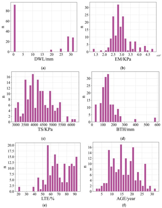
Figure 1.
Distribution of variables: (a) DWL, (b) EM, (c) TS, (d) BTH, (e) LTE, and (f) AGE.
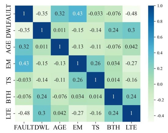
Figure 2.
Correlation between variables.
4. Model Construction
In this section, the overall process of developing the model will be explained. As shown in Figure 3, 80% of the processed data were used as the training set to train the model, while the remaining 20% were used as the test set to evaluate the performance of the model. The Bayesian hyperparameter optimization algorithm was adopted to find the optimal hyperparameters.
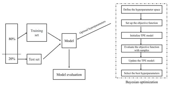
Figure 3.
The models building process.
In this study, K-fold cross-validation (K-fold CV) and the TPE method were employed to optimize hyperparameters and enhance model performance while reducing computational expenses. K-fold CV helps evaluate the generalization ability of the model across different training sets [], and the TPE algorithm automatically searches for the best combination of hyperparameters. This approach is a practical and effective technique for machine learning hyperparameter tuning, enabling significant improvements in prediction accuracy and efficiency.
K-fold CV is a robust technique for addressing the biases caused by random sampling. The training set is divided into K subsets, and the process is repeated K times. During each iteration, one subset is designated as the validation set, while the remaining K-1 subsets are utilized for training and validation. The model’s performance is assessed by averaging the results of K validations. This method of cross-validation offers the advantage of mitigating biases and variances that may arise from a single random split. It also helps to prevent issues such as overfitting and underfitting of the model. Furthermore, as depicted in Figure 4, K-fold CV aids in determining the optimal range of hyperparameters, thereby preventing wastage of computational resources due to improper parameter range settings. By systematically evaluating the model’s performance with different hyperparameter combinations, K-fold CV enables researchers to select the most suitable hyperparameters for achieving desirable results.
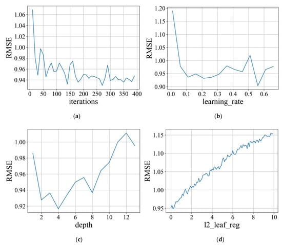
Figure 4.
Search for the optimal range of hyperparameters for the model through 5-fold cross-validation: (a) iterations, (b) learning rate, (c) depth, and (d) l2_leaf_reg.
Grid search is a widely used hyperparameter optimization method [], but it suffers from slow speed and efficiency. Although random search is more efficient than grid search, it may overlook some crucial combinations, resulting in suboptimal hyperparameter settings. Bayesian optimization, on the other hand, is less likely to miss important parameter combinations in the search space and is less prone to getting stuck in local optima. In this study, the Hyperopt library was utilized, which utilizes TPE as the surrogate function to search for the optimal combination of hyperparameters and achieve improved model performance. Hyperopt involves four parameters: space, algo, max_evals, and fn. The space parameter defines the search space by specifying the range of hyperparameters. The algo parameter represents the surrogate function model, with TPE being used in this study. The fn parameter is the objective function, which aims to minimize the RMSE of the validation set. Finally, the max_evals parameter determines the maximum number of iterations, which was set to 500 in this particular study. As shown in Table 4, the optimal hyperparameter combinations for the CatBoost model used in prediction are as follows: the optimal range for iterations is [40, 200], with an optimal value of 150; the optimal range for learning_rate is [0.01, 0.5], with an optimal value of 0.38; the optimal range for depth is [2, 10], with an optimal value of 3; and the optimal range for l2_leaf_reg is [0.01, 1], with an optimal value of 0.04.
Table 4.
Hyperparameter selection for CatBoost.
4.1. TPE-CatBoost Model Performance Evaluation
The model was trained using a specified training dataset and its predictive accuracy was evaluated using a separate test dataset. Figure 5 displays the computed R2 values of the model. The R2 value for the training dataset is as high as 0.998. Similarly, the model achieves an impressive R2 value of 0.906 on the test dataset, indicating a satisfactory level of predictive accuracy.
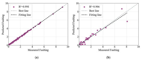
Figure 5.
A comparison of predicted and measured values for TPE-CatBoost (with 6 input variables) in the (a) training set and (b) testing set.
As shown in Figure 6, the initial R2 value of the unoptimized CatBoost model on the testing set was 0.831. The difference in accuracy before and after feature selection highlights the effectiveness of the proposed feature selection method in accurately identifying the essential variables that influence fault prediction.
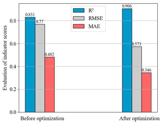
Figure 6.
A comparison between the model outcomes before and after optimization.
4.2. Models Performance Comparison
To validate the superiority of the CatBoost model, this study compared it with other commonly used models, such as RF, Adaboost, GDBT, and LightGBM algorithms. After optimizing each model (see Table 5), the prediction results were obtained for each model, as shown in Figure 7. The proposed model in this study showed the highest agreement between predicted and actual values. The performance evaluation results of each model, as shown in Table 6, indicate that the CatBoost model proposed in this study achieved the highest R2 value and the lowest RMSE and MAE values, implying its optimal overall performance.
Table 5.
Parameters used for the four benchmarked models.
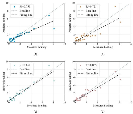
Figure 7.
Performance comparison among four benchmarked models: (a) RF model, (b) AdaBoost model, (c) GDBT model, and (d) LightGBM model.
Table 6.
Comparing the performance of five models.
4.3. SHAP-Based Feature Interpretation
One of the primary obstacles in implementing machine learning in practical business domains is the challenge of conveying the key indicators involved to operators, unlike linear regression, where this is relatively straightforward. Although the results obtained from machine learning are considered reliable, the process itself often lacks transparency and interpretability [,]. Therefore, its effectiveness and reliability need to be reviewed and validated. To solve this issue, this paper proposes the application of the SHAP interpretation method to improve model interpretability.
According to Table 7, the variable rankings based on SHAP values remain consistent in both the training and testing datasets, except for LTE and EM, which swapped positions. This indicates that the variable ranking is robust. Among all the variables, AGE has the greatest impact on faulting values, exerting over 1.5 times the influence of other significant features. The variables LTE, DWL, and EM have a moderate level of impact on faulting values. Additionally, the variables TS and BTH have a relatively less significant impact on faulting values.
Table 7.
Sorting feature importance based on SHAP.
Figure 8 shows the feature density scatter plot computed using the SHAP method. The scatter plot displays a decreasing trend in feature importance, with colors ranging from blue to red representing smaller to larger feature values. Each point represents the SHAP value of a sample, which reflects the contribution of that feature to an individual prediction, and the collection of points demonstrates the overall direction and magnitude of the feature’s influence on the prediction.
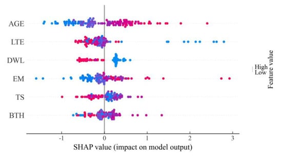
Figure 8.
Scatter plot of SHAP values.
According to the results presented in Figure 8, the analysis suggests that AGE is the most influential factor affecting the model’s predictions. As the pavement ages, both the SHAP values and faulting predictions increase. This is because over time, pavements experience prolonged load and climate conditions, resulting in accumulated displacement and frequent deformation, which is typically considered normal. Inadequate load transfer between adjacent slabs is a significant contributor to pavement faulting []. Hence, the load transfer efficiency (LTE) and dowel diameter (DWL) exhibit a negative correlation with faulting values. Moreover, the material properties of the pavement slabs, specifically the TS values, also exhibit a negative correlation with faulting. However, the study surprisingly finds a positive correlation between the elastic modulus (EM) and faulting values, contrary to common understanding. Typically, when the slabs possess higher stiffness (higher EM), critical stresses are reduced, and this helps resist faulting. One possible explanation for this positive correlation is that the EM is positively correlated with slab faulting while also negatively correlated with dowel diameter. Since dowel diameter is a primary factor in causing faulting, its impact might overshadow the influence of the elastic modulus on faulting []. Lastly, it is important to note that the pavement base layer also significantly affects the occurrence of faulting. The thickness of the pavement base layer, represented by BTH, shows a notable influence on faulting.
By utilizing the SHAP interpretation method, operators can gain insights into the extent of influence different indicators have on model predictions or outcomes. This can assist operators in understanding how various factors impact the final results and making informed decisions based on this understanding, ultimately enhancing the model’s interpretability and reliability in practical business domains.
In addition to providing global explanations for the model, SHAP provides local explanations for each individual sample. Figure 9 shows the SHAP interpretation of the prediction result for a sample with a predicted value of 0.514 mm and a true value of 0.5 mm. The figure illustrates each feature’s contribution and its value in pushing the model’s output from the baseline value, E[f(X)] (the average prediction of the CatBoost model on the entire dataset), towards the model’s output. A horizontal bar with an arrow pointing to the right represents a feature that increases the faulting value from the baseline, while an arrow pointing to the left represents a feature that decreases the faulting value. The sum of the values on the horizontal bars plus the baseline value of the sample gives the model’s output, which is the predicted faulting value for that sample.
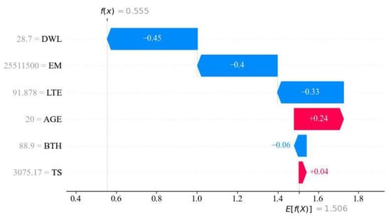
Figure 9.
SHAP for a single sample’s prediction interpretation graph.
For example, in this particular sample, the DWL is smaller than the overall average DWL of the database. Since DWL has a negative correlation with the faulting value prediction, a larger DWL has a negative effect on the prediction. The same analysis applies to other variables. It is important to note that since this figure shows the prediction result of an individual sample, the feature importance order may not be the same for each sample, and it may also differ from the overall feature ranking of the dataset.
5. Conclusions
The TPE-SHAP-CatBoost method was proposed in this study, which incorporates TPE for Bayesian hyperparameter tuning and introduces SHAP for both global and local interpretation of the model’s output. The aim is to not only train the model efficiently and accurately, but also enhance the interpretability of the model for application in practical pavement engineering practices.
- (1)
- The TPE-CatBoost model constructed with six variables demonstrated improved predictive results on the faulting test dataset. Compared to the TPE-CatBoost model constructed with 17 variables, there was an increase of 0.007 in R2, a decrease of 0.31 in MAE, and a decrease of 0.006 in RMSE. This improvement can be attributed to the capability of Boruta to identify relevant variables and eliminate unnecessary variables, thereby generating a more accurate and efficient model.
- (2)
- Compared to TPE-RF, TPE-AdaBoost, TPE-GDBT, and TPE-LightGBM, TPE-CatBoost achieved higher R2 and lower MAE and RMSE. TPE-CatBoost demonstrates greater potential for predicting Faulting.
- (3)
- By integrating with SHAP, TPE-SHAP-CatBoost can uncover the contributions of specific features to fault prediction, thereby enhancing the interpretability of the prediction results. According to the SHAP results, AGE, LTE, DWL, and EM are the most influential features affecting the output of IRI.
The proposed method provides reliable reference for pavement managers to develop specific models and improve the rigid pavement management system. Additionally, by utilizing SHAP values, pavement managers can identify which variables are more significant in predicting faulting, in order to ensure optimal pavement conditions. However, there are some limitations to be noted. Despite considering multiple variables, due to limited relevant data, some hidden variables that impact Faulting may not have been explored. Nevertheless, the method proposed in this paper has been preliminarily validated, and future research should utilize more advanced high-performance testing equipment to expand the dataset and collect more accurate and comprehensive pavement performance data, to fully unleash the potential of the model.
Author Contributions
Conceptualization, C.W. and W.X.; methodology, W.X.; software, W.X.; validation, J.L., M.G. and J.W.; investigation, C.W.; writing—original draft preparation, W.X.; writing—review and editing, W.X. All authors have read and agreed to the published version of the manuscript.
Funding
This research received no external funding.
Institutional Review Board Statement
Not applicable.
Informed Consent Statement
Not applicable.
Data Availability Statement
Data are contained within the article.
Acknowledgments
The authors would like to thank the anonymous reviewers, and the editors for their very competent comments and helpful suggestions.
Conflicts of Interest
The authors declare no conflict of interest.
References
- Naseri, H.; Ehsani, M.; Golroo, A.; Moghadas Nejad, F. Sustainable Pavement Maintenance and Rehabilitation Planning Using Differential Evolutionary Programming and Coyote Optimisation Algorithm. Int. J. Pavement Eng. 2022, 23, 2870–2887. [Google Scholar] [CrossRef]
- Augeri, M.G.; Greco, S.; Nicolosi, V. Planning Urban Pavement Maintenance by a New Interactive Multiobjective Optimization Approach. Eur. Transp. Res. Rev. 2019, 11, 17. [Google Scholar] [CrossRef]
- Mao, Z. Life-Cycle Assessment of Highway Pavement Alternatives in Aspects of Economic, Environmental, and Social Performance. Ph.D. Thesis, Texas A & M University, College Station, TX, USA, 2012. [Google Scholar]
- Hossain, M.; Gopisetti, L.S.P.; Miah, M.S. Artificial Neural Network Modelling to Predict International Roughness Index of Rigid Pavements. Int. J. Pavement Res. Technol. 2020, 13, 229–239. [Google Scholar] [CrossRef]
- Mapa, D.G.; Gunaratne, M.; Riding, K.A.; Zayed, A. Evaluating Early-Age Stresses in Jointed Plain Concrete Pavement Repair Slabs. ACI Mater. J. 2020, 117, 119–132. [Google Scholar]
- Wang, C.; Xiao, W.; Liu, J. Developing an Improved Extreme Gradient Boosting Model for Predicting the International Roughness Index of Rigid Pavement. Constr. Build. Mater. 2023, 408, 133523. [Google Scholar] [CrossRef]
- Simpson, A.L.; National Research Council; Jordahl, P.R.; Owusu-Antwi, E. Sensitivity Analyses for Selected Pavement Distresses; Strategic Highway Research Program, SHRP-P; National Research Council: Washington, DC, USA, 1994; ISBN 978-0-309-05771-4. [Google Scholar]
- Yu, H.T.; Smith, K.D.; Darter, M.I.; Jiang, J. Performance of Concrete Pavements, Volume III: Improving Concrete Pavement Performance (No. FHWA-RD-95-111); Department of Transportation, Federal Highway Administration: Washington, DC, USA, 1998. [Google Scholar]
- Ker, H.-W.; Lee, Y.-H.; Lin, C.-H. Development of Faulting Prediction Models for Rigid Pavements Using LTPP Database. Statistics 2008, 218, 0037-0030. [Google Scholar]
- Saghafi, B.; Hassaniz, A.; Noori, R.; Bustos, M.G. Artificial neural networks and regression analysis for predicting faulting in jointed concrete pavements considering base condition. Int. J. Pavement Res. Technol. 2009, 2, 20–25. [Google Scholar]
- Wang, W.-N.; Tsai, Y.-C.J. Back-Propagation Network Modeling for Concrete Pavement Faulting Using LTPP Data. Int. J. Pavement Res. Technol. 2013, 6, 651–657. [Google Scholar] [CrossRef]
- Ehsani, M.; Moghadas Nejad, F.; Hajikarimi, P. Developing an Optimized Faulting Prediction Model in Jointed Plain Concrete Pavement Using Artificial Neural Networks and Random Forest Methods. Int. J. Pavement Eng. 2022, 1–16. [Google Scholar] [CrossRef]
- Ehsani, M.; Hamidian, P.; Hajikarimi, P.; Moghadas Nejad, F. Optimized Prediction Models for Faulting Failure of Jointed Plain Concrete Pavement Using the Metaheuristic Optimization Algorithms. Constr. Build. Mater. 2023, 364, 129948. [Google Scholar] [CrossRef]
- Kursa, M.B.; Rudnicki, W.R. Feature Selection with the Boruta Package. J. Stat. Softw. 2010, 36, 1–13. [Google Scholar] [CrossRef]
- Jia, D.; Yang, L.; Gao, X.; Li, K. Assessment of a New Solar Radiation Nowcasting Method Based on FY-4A Satellite Imagery, the McClear Model and SHapley Additive exPlanations (SHAP). Remote Sens. 2023, 15, 2245. [Google Scholar] [CrossRef]
- Chen, B.; Zheng, H.; Luo, G.; Chen, C.; Bao, A.; Liu, T.; Chen, X. Adaptive Estimation of Multi-Regional Soil Salinization Using Extreme Gradient Boosting with Bayesian TPE Optimization. Int. J. Remote Sens. 2022, 43, 778–811. [Google Scholar] [CrossRef]
- Kavzoglu, T.; Teke, A. Advanced Hyperparameter Optimization for Improved Spatial Prediction of Shallow Landslides Using Extreme Gradient Boosting (XGBoost). Bull. Eng. Geol. Environ. 2022, 81, 201. [Google Scholar] [CrossRef]
- Yu, J.; Zheng, W.; Xu, L.; Meng, F.; Li, J.; Zhangzhong, L. TPE-CatBoost: An Adaptive Model for Soil Moisture Spatial Estimation in the Main Maize-Producing Areas of China with Multiple Environment Covariates. J. Hydrol. 2022, 613, 128465. [Google Scholar] [CrossRef]
- Behkamal, B.; Entezami, A.; De Michele, C.; Arslan, A.N. Investigation of Temperature Effects into Long-Span Bridges via Hybrid Sensing and Supervised Regression Models. Remote Sens. 2023, 15, 3503. [Google Scholar] [CrossRef]
- Merow, C.; Smith, M.J.; Edwards Jr, T.C.; Guisan, A.; McMahon, S.M.; Normand, S.; Thuiller, W.; Wüest, R.O.; Zimmermann, N.E.; Elith, J. What Do We Gain from Simplicity versus Complexity in Species Distribution Models? Ecography 2014, 37, 1267–1281. [Google Scholar] [CrossRef]
- Belanche-Muñoz, L.; Blanch, A.R. Machine Learning Methods for Microbial Source Tracking. Environ. Model. Softw. 2008, 23, 741–750. [Google Scholar] [CrossRef]
- Yang, E.; Yang, Q.; Li, J.; Zhang, H.; Di, H.; Qiu, Y. Establishment of Icing Prediction Model of Asphalt Pavement Based on Support Vector Regression Algorithm and Bayesian Optimization. Constr. Build. Mater. 2022, 351, 128955. [Google Scholar] [CrossRef]
- Grinsztajn, L.; Oyallon, E.; Varoquaux, G. Why Do Tree-Based Models Still Outperform Deep Learning on Typical Tabular Data? Adv. Neural Inf. Process. Syst. 2022, 35, 507–520. [Google Scholar]
- Hancock, J.; Khoshgoftaar, T. CatBoost for Big Data: An Interdisciplinary Review. J. Big Data 2020, 7, 94. [Google Scholar] [CrossRef] [PubMed]
- Prokhorenkova, L.; Gusev, G.; Vorobev, A.; Dorogush, A.V.; Gulin, A. CatBoost: Unbiased Boosting with Categorical Features. Adv. Neural Inf. Process. Syst. 2018, 31. [Google Scholar]
- Lundberg, S.M.; Lee, S.-I. A Unified Approach to Interpreting Model Predictions. Adv. Neural Inf. Process. Syst. 2017, 30. [Google Scholar]
- Lundberg, S.M.; Erion, G.; Chen, H.; DeGrave, A.; Prutkin, J.M.; Nair, B.; Katz, R.; Himmelfarb, J.; Bansal, N.; Lee, S.-I. From Local Explanations to Global Understanding with Explainable AI for Trees. Nat. Mach. Intell. 2020, 2, 56–67. [Google Scholar] [CrossRef] [PubMed]
- Moncada-Torres, A.; van Maaren, M.C.; Hendriks, M.P.; Siesling, S.; Geleijnse, G. Explainable Machine Learning Can Outperform Cox Regression Predictions and Provide Insights in Breast Cancer Survival. Sci. Rep. 2021, 11, 6968. [Google Scholar] [CrossRef] [PubMed]
- Jung, Y. Multiple Predicting K-Fold Cross-Validation for Model Selection. J. Nonparametr. Stat. 2018, 30, 197–215. [Google Scholar] [CrossRef]
- Bergstra, J.; Bengio, Y. Random Search for Hyper-Parameter Optimization. J. Mach. Learn. Res. 2012, 13, 281–305. [Google Scholar]
- Van den Broeck, G.; Lykov, A.; Schleich, M.; Suciu, D. On the Tractability of SHAP Explanations. J. Artif. Intell. Res. 2022, 74, 851–886. [Google Scholar] [CrossRef]
- Lin, N.; Zhang, D.; Feng, S.; Ding, K.; Tan, L.; Wang, B.; Chen, T.; Li, W.; Dai, X.; Pan, J.; et al. Rapid Landslide Extraction from High-Resolution Remote Sensing Images Using SHAP-OPT-XGBoost. Remote Sens. 2023, 15, 3901. [Google Scholar] [CrossRef]
- Chen, Y.; Lytton, R.L. Development of a New Faulting Model in Jointed Concrete Pavement Using LTPP Data. Transp. Res. Rec. 2019, 2673, 407–417. [Google Scholar] [CrossRef]
- Chen, Y.; Lytton, R.L. Exploratory Analysis of LTPP Faulting Data Using Statistical Techniques. Constr. Build. Mater. 2021, 309, 125025. [Google Scholar] [CrossRef]
Disclaimer/Publisher’s Note: The statements, opinions and data contained in all publications are solely those of the individual author(s) and contributor(s) and not of MDPI and/or the editor(s). MDPI and/or the editor(s) disclaim responsibility for any injury to people or property resulting from any ideas, methods, instructions or products referred to in the content. |
© 2023 by the authors. Licensee MDPI, Basel, Switzerland. This article is an open access article distributed under the terms and conditions of the Creative Commons Attribution (CC BY) license (https://creativecommons.org/licenses/by/4.0/).