
A Bearing Fault Diagnosis Method Based on Dilated Convolution and Multi-Head Self-Attention Mechanism

Abstract
:1. Introduction
2. Relevant Methodology
2.1. Convolutional Neural Networks (CNNs)
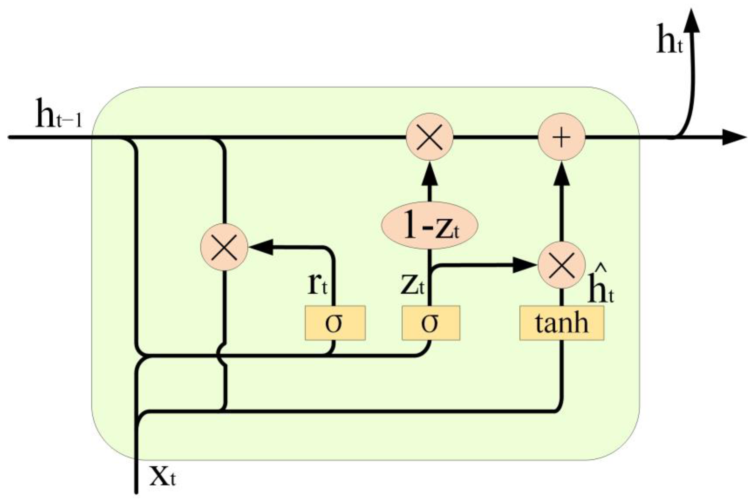
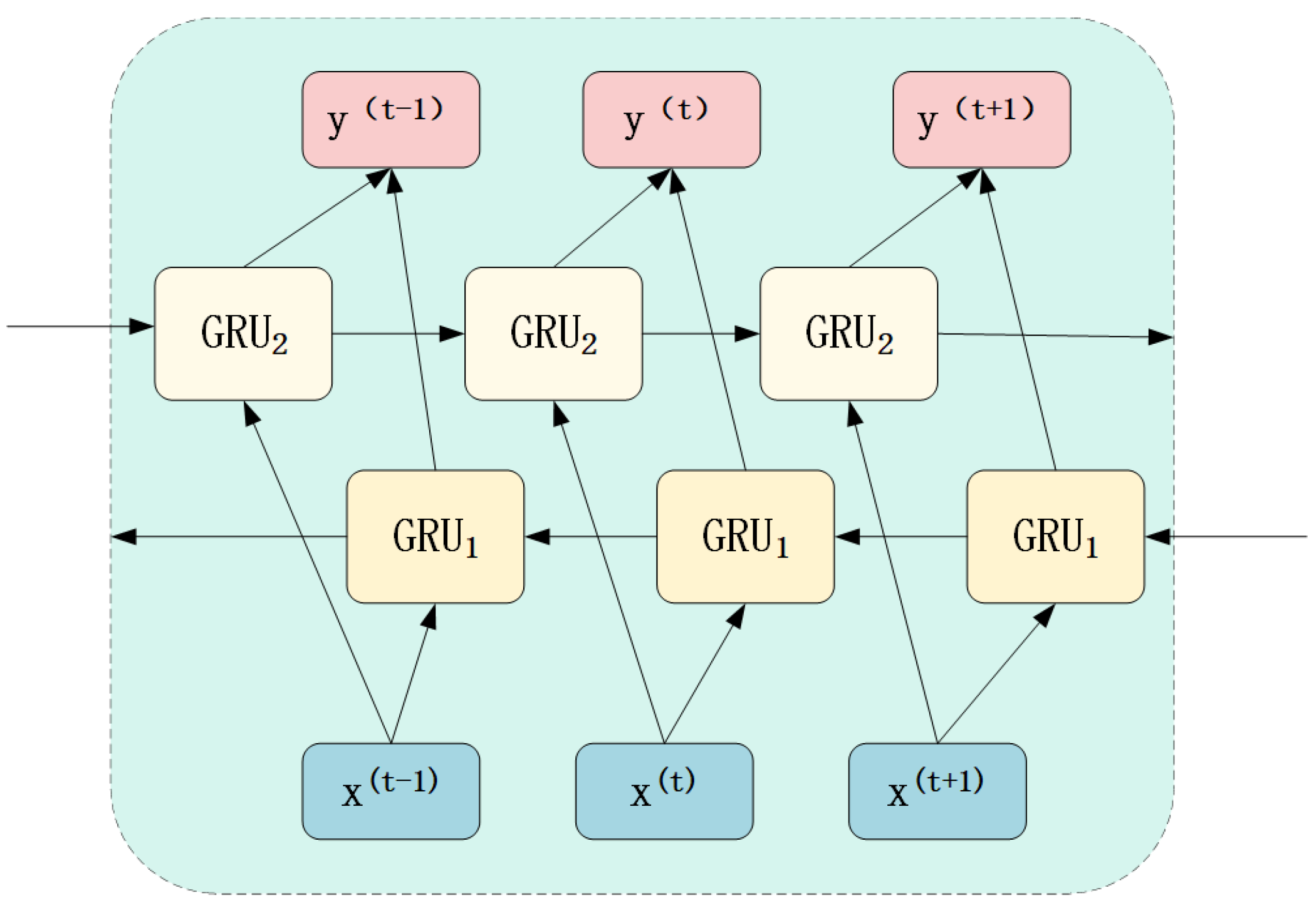
2.2. GRU
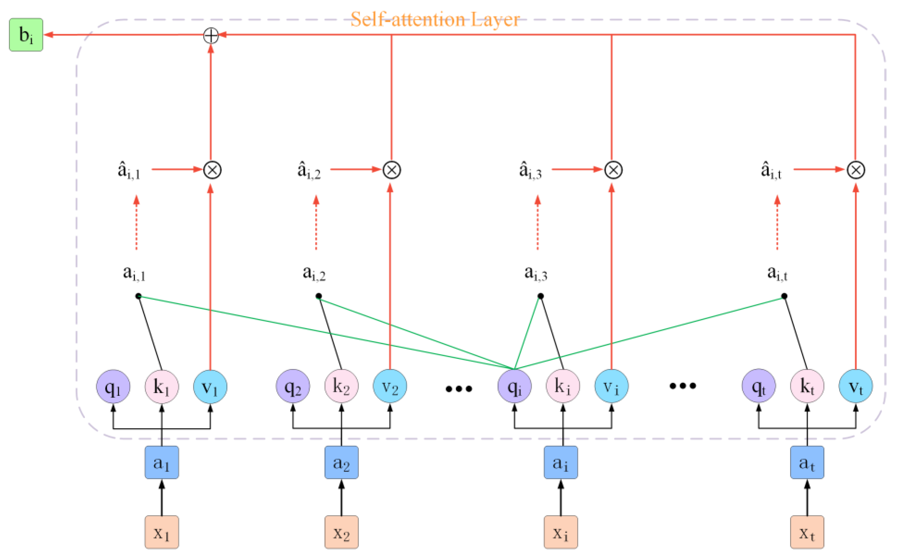
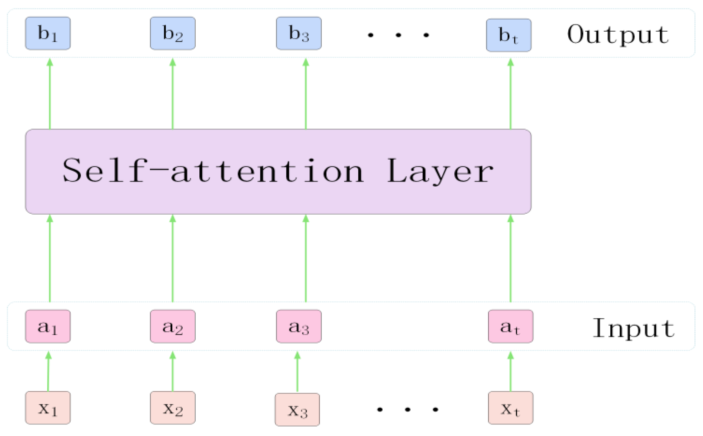
2.3. Self-Attention Mechanism
3. Detailed Methods
3.1. ACN
3.2. Improved ReLU Functions
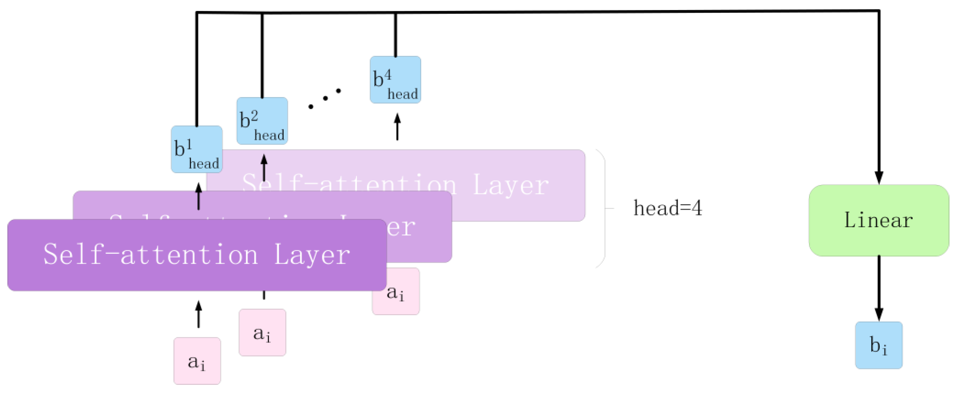
3.3. Multi-Head Self-Attention Mechanism
3.4. ACN_BM Model
4. Experimental Demonstration
4.1. Experimental Dataset
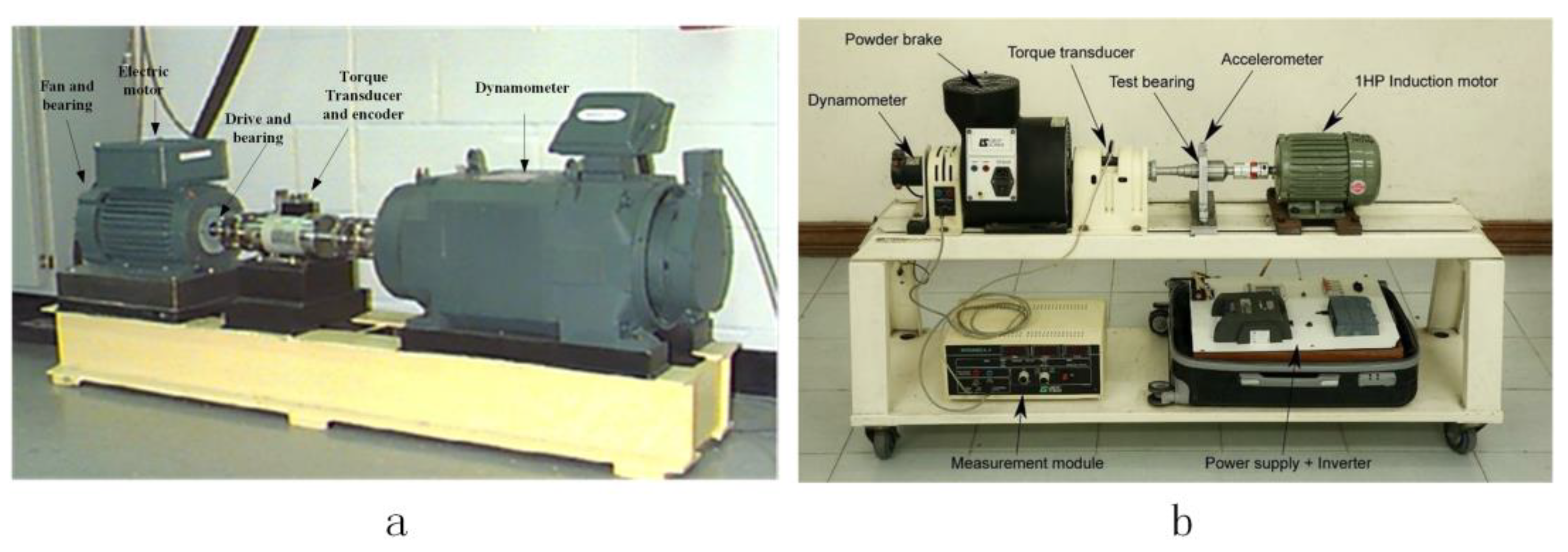
4.1.1. CWRU Dataset
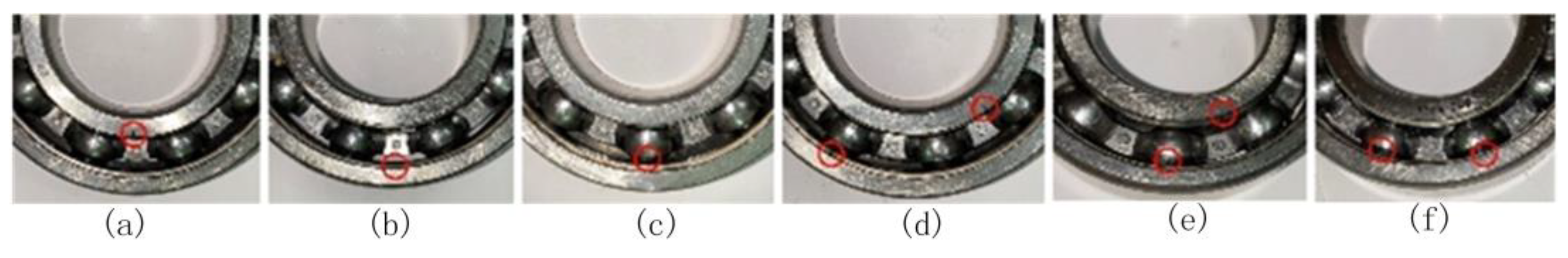
4.1.2. HUST Dataset
4.2. Test Scheme
- In the initial validation of the model performance using the CWRU dataset, we needed to perform data enhancement on the CWRU dataset due to its lesser amount of data than that of other datasets. We used sliding window sampling here to increase each sample type to 800. To verify the model’s training effect on different bearings under complex working conditions, we divided the data into 12 classes. Subsequently, it was necessary to juxtapose various models to exemplify the model’s efficiency and include ablation experiments to corroborate the indispensability of each segment within the model.
- The HUST dataset was sufficiently sampled, and no data enhancement was performed. Here, the data were divided into seven categories in total, and for the sake of experimental rigor, we set all other variables as the same. Finally, we also compared five models to prove that the model has made some modest contributions to the academic community in the face of the fault recognition rate of five types of bearings.
- In actual operational settings, the model for diagnosing faults within rotating machinery has to confront the noise produced by the mutual oscillations and abrasion amongst the machine’s components. Such conditions make the vibration signals detected by the sensors susceptible to noise pollution, resulting in a blurring of the fault details contained within these signals. According to the survey, the noise of the diagnostic signal is generally additive white Gaussian noise [36]. Therefore, in this paper, different levels of additive white Gaussian noise were added to the test set’s signals to test the trained model’s anti-noise performance.
4.3. Test Setting
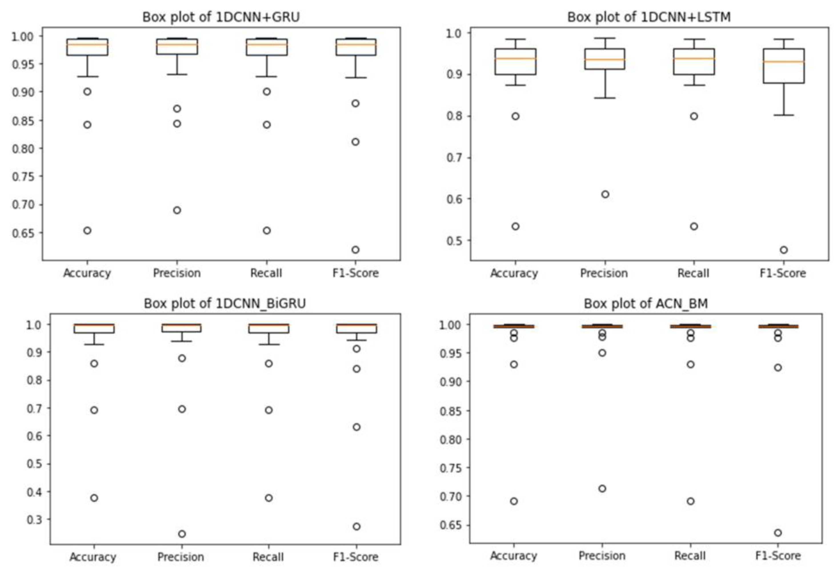
4.4. Result
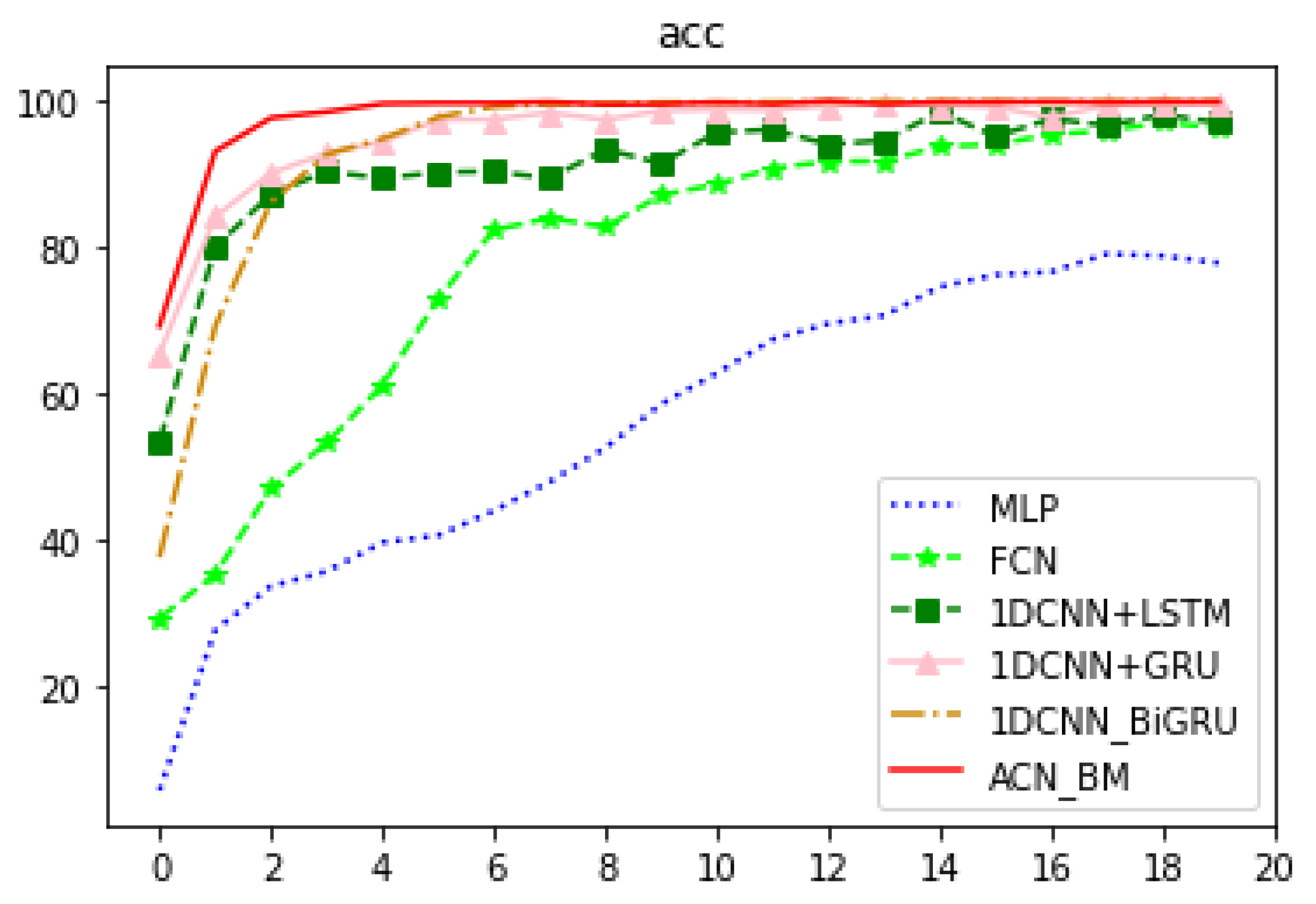
4.4.1. Experiment I: Preliminary Experiments on the CWRU Dataset
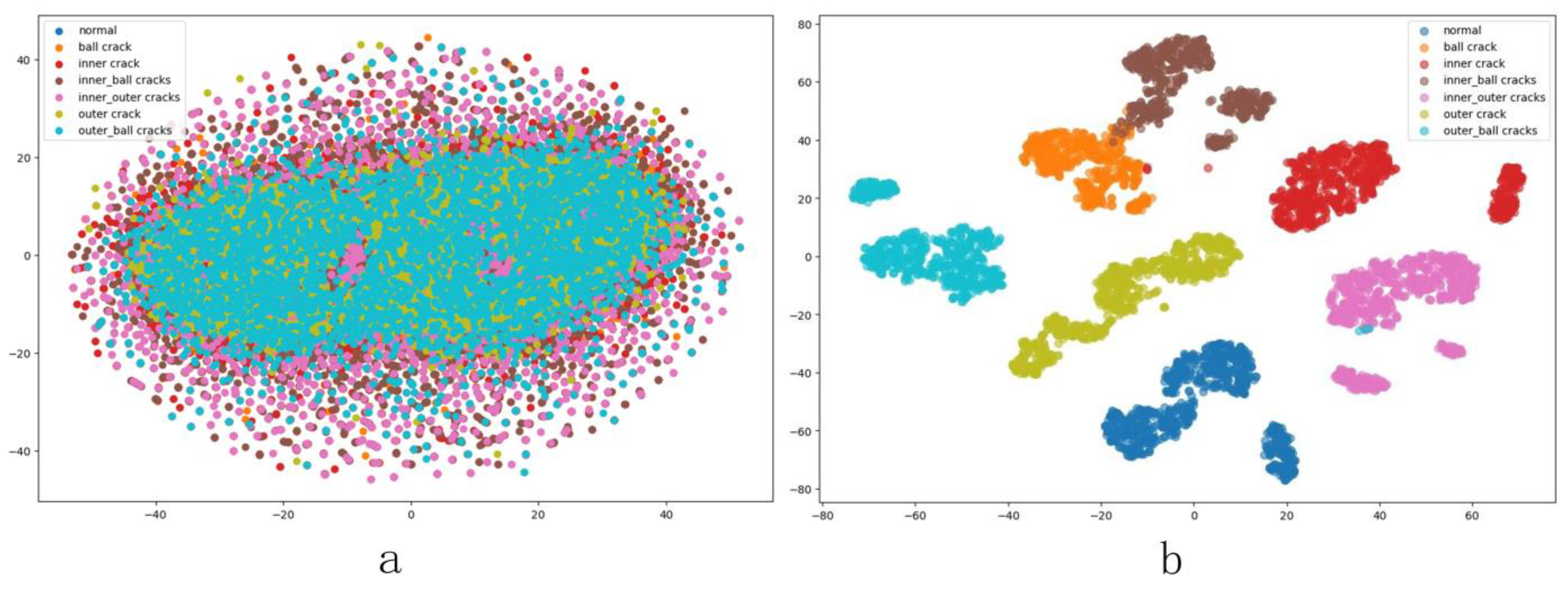
4.4.2. Experiment II: To Verify the Performance of the Model on Different Bearings
4.4.3. Experiment III: Noise Immunity Experiment of the Model
5. Discussion
6. Conclusions
Author Contributions
Funding
Institutional Review Board Statement
Informed Consent Statement
Data Availability Statement
Conflicts of Interest
References
- Nandi, S.; Toliyat, H.A.; Li, X. Condition Monitoring and Fault Diagnosis of Electrical Motors—A Review. IEEE Trans. Energy Convers. 2005, 20, 719–729. [Google Scholar] [CrossRef]
- Mohammad-Alikhani, A.; Pradhan, S.; Dhale, S.; Mobarakeh, B.N. A Variable Speed Fault Detection Approach for Electric Motors in EV Applications based on STFT and RegNet. In Proceedings of the 2023 IEEE Transportation Electrification Conference & Expo (ITEC), Detroit, MI, USA, 21–23 June 2023; pp. 1–5. [Google Scholar]
- Alonso-González, M.; Díaz, V.G.; Pérez, B.L.; G-Bustelo, B.C.P.; Anzola, J.P. Bearing Fault Diagnosis with Envelope Analysis and Machine Learning Approaches Using CWRU Dataset. IEEE Access 2023, 11, 57796–57805. [Google Scholar] [CrossRef]
- Zou, X.-L.; Han, K.-X.; Chien, W.; Gan, X.-Y.; Shi, L.-Y. Overview of Bearing Fault Diagnosis Based on Deep Learning. In Proceedings of the 2023 IEEE 3rd International Conference on Electronic Communications, Internet of Things and Big Data (ICEIB), Taichung, Taiwan, 14–16 April 2023; pp. 324–326. [Google Scholar]
- Brigham, E.O.; Morrow, R.E. The fast Fourier transform. IEEE Spectr. 1967, 4, 63–70. [Google Scholar] [CrossRef]
- Donnelly, D. The Fast Fourier and Hilbert-Huang Transforms: A Comparison. In Proceedings of the Multiconference on Computational Engineering in Systems Applications, Beijing, China, 4–6 October 2006; pp. 84–88. [Google Scholar]
- Yin, P.; Nie, J.; Liang, X.; Yu, S.; Wang, C.; Nie, W.; Ding, X. A Multiscale Graph Convolutional Neural Network Framework for Fault Diagnosis of Rolling Bearing. IEEE Trans. Instrum. Meas. 2023, 72, 1–13. [Google Scholar] [CrossRef]
- Al-Tashi, Q.; Kadir, S.J.A.; Rais, H.M.; Mirjalili, S.; Alhussian, H. Binary Optimization Using Hybrid Grey Wolf Optimization for Feature Selection. IEEE Access 2019, 7, 39496–39508. [Google Scholar] [CrossRef]
- Dahan, F.; El Hindi, K.; Ghoneim, A.; Alsalman, H. An Enhanced Ant Colony Optimization Based Algorithm to Solve QoS-Aware Web Service Composition. IEEE Access 2021, 9, 34098–34111. [Google Scholar] [CrossRef]
- Jin, N.; Rahmat-Samii, Y. Advances in Particle Swarm Optimization for Antenna Designs: Real-Number, Binary, Single-Objective and Multiobjective Implementations. IEEE Trans. Antennas Propag. 2007, 55, 556–567. [Google Scholar] [CrossRef]
- Lee, C.-Y.; Le, T.-A.; Lin, Y.-T. A feature selection approach hybrid grey wolf and heap-based optimizer applied in bearing fault diagnosis. IEEE Access 2022, 10, 56691–56705. [Google Scholar] [CrossRef]
- Kwon, B.; Kim, J.; Lee, K.; Lee, Y.K.; Park, S.; Lee, S. Implementation of a virtual training simulator based on 360° multi-view human action recognition. IEEE Access 2017, 5, 12496–12511. [Google Scholar] [CrossRef]
- NMohamed, N.; Baskaran, N.K.; Patil, P.P.; Alatba, S.R.; Aich, S.C. Thermal Images Captured and Classifier-based Fault Detection System for Electric Motors Through ML Based Model. In Proceedings of the 2023 3rd International Conference on Advance Computing and Innovative Technologies in Engineering (ICACITE), Greater Noida, India, 12–13 May 2023; pp. 649–654. [Google Scholar]
- Tian, J.; Morillo, C.; Azarian, M.H.; Pecht, M. Motor Bearing Fault Detection Using Spectral Kurtosis-Based Feature Extraction Coupled With K-Nearest Neighbor Distance Analysis. IEEE Trans. Ind. Electron. 2016, 63, 1793–1803. [Google Scholar] [CrossRef]
- Chen, J.; Hu, W.; Cao, D.; Zhang, M.; Huang, Q.; Chen, Z.; Blaabjerg, F. Novel data-driven approach based on capsule network for intelligent multi-fault detection in electric motors. IEEE Trans. Energy Convers. 2020, 36, 2173–2184. [Google Scholar] [CrossRef]
- Liu, Y.; Wen, W.; Bai, Y.; Meng, Q. Self-supervised feature extraction via time–frequency contrast for intelligent fault diagnosis of rotating machinery. Measurement 2023, 210, 112551. [Google Scholar] [CrossRef]
- Chen, Y.; Xiao, L.; Li, Z. Partial Domain Fault Diagnosis of Bearings under Cross-Speed Conditions Based on 1D-CNN. In Proceedings of the 2022 Global Reliability and Prognostics and Health Management (PHM-Yantai), Yantai, China, 13–16 October 2022; pp. 1–8. [Google Scholar]
- Cheng, Q.; Peng, B.; Li, Q.; Liu, S. A rolling bearing fault diagnosis model based on WCNN-BiGRU. In Proceedings of the 2021 China Automation Congress (CAC), Beijing, China, 22–24 October 2021; pp. 3368–3372. [Google Scholar]
- Guo, L.; Zhang, S.; Huang, Q. Rolling bearing fault diagnosis based on the combination of improved deep convolution network and gated recurrent unit. In Proceedings of the 2022 34th Chinese Control and Decision Conference (CCDC), Hefei, China, 22–24 October 2022; pp. 1473–1478. [Google Scholar]
- Xu, P.; Zhang, L. A Fault Diagnosis Method for Rolling Bearing Based on 1D-ViT Model. IEEE Access 2023, 11, 39664–39674. [Google Scholar] [CrossRef]
- Cheng, L.; Dong, Z.; Wang, S.; Zhang, J.; Chen, J. Based on improved one-dimensional convolutional neural network analysis of the rolling bearing fault diagnosis. J. Mech. Des. Res. 2023, 6, 126–130. [Google Scholar]
- Thuan, N.D.; Hong, H.S. HUST bearing: A practical dataset for ball bearing fault diagnosis. BMC Res. Notes 2023, 16, 138. [Google Scholar] [CrossRef]
- Smith, W.A.; Randall, R.B. Rolling element bearing diagnostics using the Case Western Reserve University data: A benchmark study. Mech. Syst. Signal Process. 2015, 64–65, 100–131. [Google Scholar] [CrossRef]
- Zhang, Y.; Yao, L.; Zhang, L.; Luo, H. Fault diagnosis of natural gas pipeline leakage based on 1D-CNN and self-attention mechanism. In Proceedings of the 2022 IEEE 6th Advanced Information Technology, Electronic and Automation Control Conference (IAEAC), Beijing, China, 3–5 October 2022; pp. 1282–1286. [Google Scholar]
- Li, X.; Zhang, W.; Ding, Q. Understanding and improving deep learning-based rolling bearing fault diagnosis with attention mechanism. Signal Process. 2019, 161, 136–154. [Google Scholar] [CrossRef]
- Fukushima, K. Neocognitron: A self-organizing neural network model for a mechanism of pattern recognition unaffected by shift in position. Biol. Cybern. 1980, 36, 193–202. [Google Scholar] [CrossRef]
- Kayed, M.; Anter, A.; Mohamed, H. Classification of Garments from Fashion MNIST Dataset Using CNN LeNet-5 Architecture. In Proceedings of the 2020 International Conference on Innovative Trends in Communication and Computer Engineering (ITCE), Aswan, Egypt, 8–9 February 2020; pp. 238–243. [Google Scholar]
- Zhang, J.; Sun, Y.; Guo, L.; Gao, H.; Hong, X.; Song, H. A new bearing fault diagnosis method based on modified convolutional neural networks. Chin. J. Aeronaut. 2020, 33, 439–447. [Google Scholar] [CrossRef]
- Shao, X.; Kim, C.-S. Unsupervised Domain Adaptive 1D-CNN for Fault Diagnosis of Bearing. Sensors 2022, 22, 4156. [Google Scholar] [CrossRef]
- Graves, A. Long short-term memory. In Supervised Sequence Labeling with Recurrent Neural Networks; Springer: Berlin/Heidelberg, Germany, 2012; pp. 37–45. [Google Scholar]
- Choe, D.E.; Kim, H.C.; Kim, M.H. Sequence-based modeling of deep learning with LSTM and GRU networks for structural damage detection of floating offshore wind turbine blades. Renew. Energy 2021, 174, 218–235. [Google Scholar] [CrossRef]
- Liu, Z. Bearing Fault Diagnosis of End-to-End Model Design Based on 1DCNN-GRU Network. Discret. Dyn. Nat. Soc. 2022, 2022, 7167821. [Google Scholar]
- Yang, Y.C.; Liu, T.; Liu, X.Q. One dimensional convolution neural network fault diagnosis of planetary gearbox based on attention mechanism. Mach. Electron. 2021, 39, 3–8. [Google Scholar]
- Shao, S.; McAleer, S.; Yan, R.; Baldi, P. Highly accurate machine fault diagnosis using deep transfer learning. IEEE Trans. Ind. Informat. 2019, 15, 2446–2455. [Google Scholar] [CrossRef]
- Yang, X.; Xiao, Y. Named Entity Recognition Based on BERT-MBiGRU-CRF and Multi-head Self-attention Mechanism. In Proceedings of the 2022 4th International Conference on Natural Language Processing (ICNLP), Xi’an, China, 25–27 March 2022; pp. 178–183. [Google Scholar]
- Amar, M.; Gondal, I.; Wilson, C. Vibration spectrum imaging: A novel bearing fault classification approach. IEEE Trans. Ind. Electron. 2015, 62, 494–502. [Google Scholar] [CrossRef]


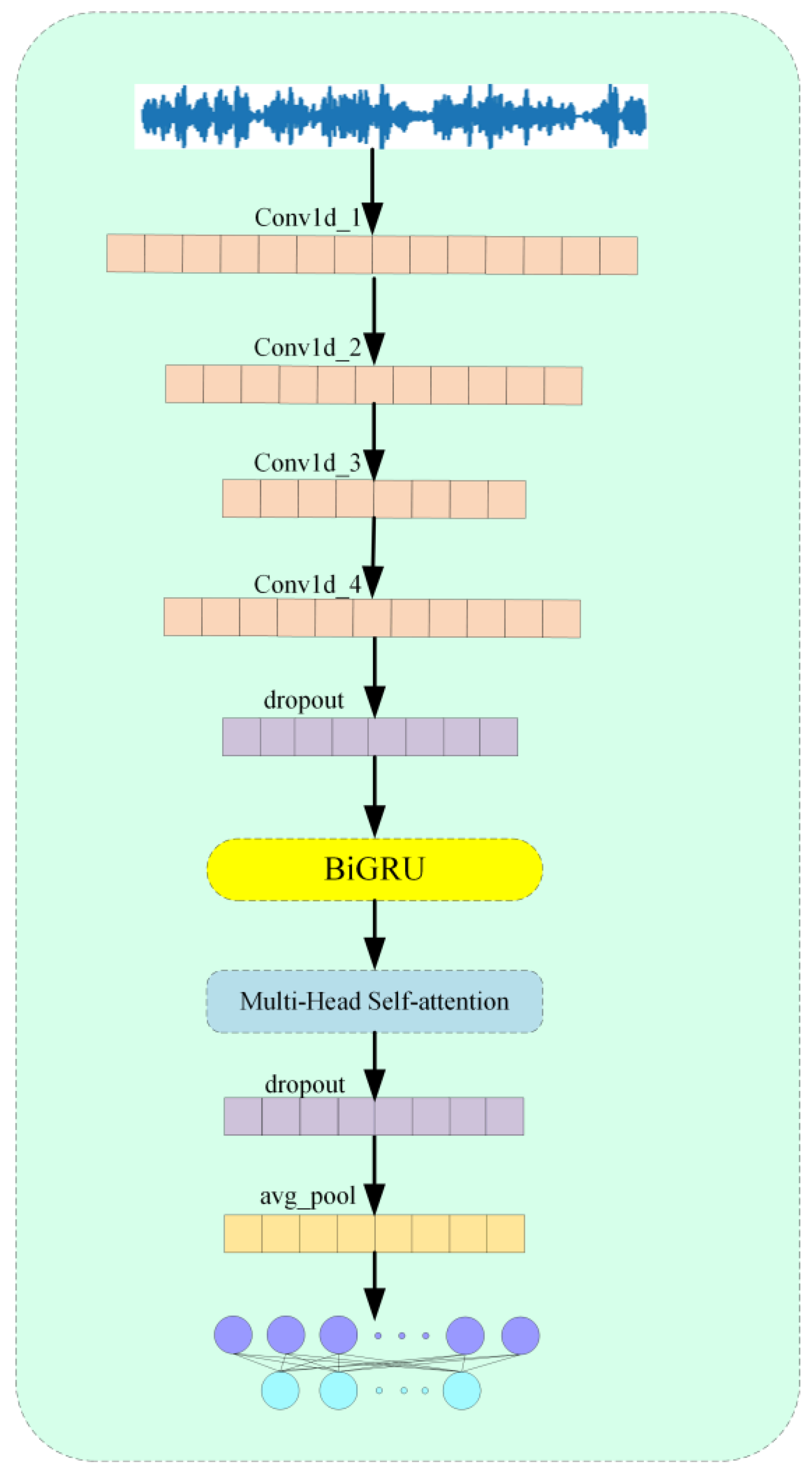
| Network Layer | Kernel_Size/Strid | Parameter | Input Size | Input Size |
|---|---|---|---|---|
| Conv1d | 7/1 | 2 | (1, 2048) | (64, 2048) |
| Conv1d | 3/1 | 2 | (64, 2048) | (128, 2048) |
| Conv1d | 3/1 | 2 | (128, 1024) | (256, 1024) |
| Conv1d | 3/1 | 2 | (256, 512) | (128, 512) |
| Dropout | - | 0.3 | (128, 256) | (128, 256) |
| BiGRU | - | 128 | (128, 256) | (128, 256) |
| Dropout | 0.5 | (128, 256) | (128, 256) | |
| Multi-Head Self-attention | - | 4 | (128, 256) | (128, 256) |
| Avg_pool | - | (256, 128) | (256) | |
| Fc | - | (256) | (7) |
| Dataset | Accuracy % | 1DCNN+LSTM | 1DCNN+GRU | 1DCNN+BiGRU | ACN_BM |
|---|---|---|---|---|---|
| HUST | Training-set | 0.23 | 0.14 | 0.09 | 99.89 0.06 |
| test-set | 0.35 | 0.36 | 0.21 | 0.15 | |
| CWRU | Training-set | 0.33 | 0.26 | 96.24 0.11 | 0.21 |
| test-set | 0.29 | 0.49 | 0.57 | 98.64 0.16 |
| Head numbers | 1 | 2 | 4 | 8 | 1 | 2 | 4 | 8 |
| SNR | 0 | 0 | 0 | 0 | −8 | −8 | −8 | −8 |
| Average precision | 98.7% | 98.76% | 98.83% | 98.94% | 86.87% | 88.32% | 89.62% | 89.92% |
| Final learning rate | 0.0001 | 0.000001 | 0.000001 | 0.000001 | 0.0001 | 0.000001 | 0.000001 | 0.000001 |
Disclaimer/Publisher’s Note: The statements, opinions and data contained in all publications are solely those of the individual author(s) and contributor(s) and not of MDPI and/or the editor(s). MDPI and/or the editor(s) disclaim responsibility for any injury to people or property resulting from any ideas, methods, instructions or products referred to in the content. |
© 2023 by the authors. Licensee MDPI, Basel, Switzerland. This article is an open access article distributed under the terms and conditions of the Creative Commons Attribution (CC BY) license (https://creativecommons.org/licenses/by/4.0/).
Share and Cite
Hou, P.; Zhang, J.; Jiang, Z.; Tang, Y.; Lin, Y. A Bearing Fault Diagnosis Method Based on Dilated Convolution and Multi-Head Self-Attention Mechanism. Appl. Sci. 2023, 13, 12770. https://doi.org/10.3390/app132312770
Hou P, Zhang J, Jiang Z, Tang Y, Lin Y. A Bearing Fault Diagnosis Method Based on Dilated Convolution and Multi-Head Self-Attention Mechanism. Applied Sciences. 2023; 13(23):12770. https://doi.org/10.3390/app132312770
Chicago/Turabian StyleHou, Peng, Jianjie Zhang, Zhangzheng Jiang, Yiyu Tang, and Ying Lin. 2023. "A Bearing Fault Diagnosis Method Based on Dilated Convolution and Multi-Head Self-Attention Mechanism" Applied Sciences 13, no. 23: 12770. https://doi.org/10.3390/app132312770
APA StyleHou, P., Zhang, J., Jiang, Z., Tang, Y., & Lin, Y. (2023). A Bearing Fault Diagnosis Method Based on Dilated Convolution and Multi-Head Self-Attention Mechanism. Applied Sciences, 13(23), 12770. https://doi.org/10.3390/app132312770