Wheat Quantity Monitoring Methods Based on Inventory Measurement and SVR Prediction Model

Abstract

Due to the influences of the storage environment, water content change, particle settlement, natural loss, and other factors, the distribution density of wheat and the volume of grain pile in the storage process are gradually changed so that the single weight calculation method cannot objectively evaluate the storage quantity of wheat and also causes difficulties to the regular inspection of the quantity of wheat stock. To meet the practical needs of wheat inventory monitoring, a wheat inventory monitoring method based on inventory measurement and the support vector machine regression (SVR) prediction model is proposed. By collecting the working papers for the physical inspection of wheat in grain warehouses in Shanxi province, Hebei province, Henan province, Jiangsu province, and other places, the storage time, storage weight, storage moisture content, measured moisture content, measured volume weight, measured net volume, and measured weight for inspection were selected as training samples for the SVR prediction model, and kernel function selection and parameter optimization were carried out. We developed an optimal prediction model for the amount of wheat in the grain depots. In the actual grain store measurement process, the net volume of wheat in the current grain store was obtained by a laser volumetric measuring apparatus, the actual bulk density of wheat was sampled, and the actual moisture content of wheat was measured by sampling. The three samples, their storage time, their storage moisture content, and their storage weight were fed into the trained SVR prediction model as new samples, and the predicted weight of the wheat in the current grain store was obtained from the output. The error rate calculation procedure was introduced to achieve an anomalous judgment error rate for grain depots. The experimental results showed that the SVR prediction model based on the linear kernel function had a very low mean squared error and high determination coefficient, and the average prediction accuracy of the grain stock error rate reached 93.2 percent, which can meet the requirements of wheat quantity monitoring in grain warehouses.

1. Introduction

Grain is an important strategic material for national stability and development. Ensuring food security is a long-term strategic task for our country that directly affects national security [1]. To ensure that grain can meet the needs of the people and respond to emergencies, China has set up a three-tier grain storage system with nearly 10,000 grain warehouses at all levels, and the existing grain storage capacity has reached 500 million tons [2]. In order to strengthen the supervision and inspection of the amount of grain stored in grain depots and to ensure the authenticity and reliability of the amount of grain stored in grain depots, it is important to study the amount of grain stored in grain depots. Because wheat has excellent storage resistance, the storage time can reach 3–5 years under normal temperature conditions, and the storage time at low temperature (15 ℃) can reach 5–8 years; thus, the existing medium and long-term grain storage in China is mainly wheat. However, the grain volume in the grain store gradually changes during wheat storage due to storage environment, changes in water content, grain settling, natural losses, and other factors, which makes grain quantity inspection difficult. Inventory and spot checks mainly rely on traditional manual methods for inspection and auditing, which have problems of low efficiency and high cost [3,4]. To address these issues, researchers in relevant fields have conducted extensive research and made numerous attempts. As a result, various technologies for monitoring the quantity of grain in granaries are continuously emerging, playing a crucial role in safeguarding national food security [5].

Currently, there are two primary methods for monitoring the quantity of grain in granaries: direct measurement and indirect measurement [6]. The direct measurement method involves manual weighing and pressure sensor measurement. The grain depot is quite large, with each warehouse capable of storing close to 10,000 tons of grain. However, there is currently no sensor available that can accurately weigh the grain at the bottom of the granary. The pressure sensor method involves placing numerous pressure sensors throughout the grain bin to measure the pressure of grain on the side walls and bottom. By using the conversion relationship between pressure and gravity on the grain in the bin, the quantity of grain can be determined [7,8,9]. However, it is important to note the Janssen effect, which states that when the grain piles in the granary reach a certain height, the force at the bottom of the granary no longer increases with the addition of more grain. While the pressure sensor method takes into account the influence of sidewall pressure, its effectiveness still needs to be verified. Although many scholars have carried out a lot of research on the granary weighing measurement method, there is still no major breakthrough and no feasible plan for practical application.

The indirect measurement method involves using different technical means to measure the volume of grain silos and then combining it with grain density to determine the quantity of grain indirectly. Various technologies are employed in this method, such as 3D laser scanning, ultrasonic measurement, electromagnetic wave detection, wide-beam radar detection, and machine vision detection. The electromagnetic wave detection method involves using a radar antenna placed on the surface of a grain pile to scan the entire surface horizontally. This allows for the detection of internal granaries by analyzing the signals reflected from electromagnetic wave targets [10,11]. However, this method must take into account various factors such as grain type, temperature, and impurity content. To enhance the accuracy of the measurement data, it is important to continuously establish a real-time model that relates grain density to the dielectric constant. Additionally, there are specific requirements for the electronic equipment used in the measurement process, and challenges related to the depth of antenna insertion in the grain pile and the alignment between antennas must be addressed. Further research is needed to assess the practicality of this method [12,13]. The wide-beam radar detection method utilizes three antennas to acquire the Cartesian coordinates of strong scattering points on the surface of a grain pile. This method also gathers three-dimensional height information and calculates the corresponding grain volume using the relevant formula [14]. However, the measurement of grain volume is greatly influenced by the reflection of the wall facing the radar wave in the closed space of the granary. This necessitates the removal of numerous anomalies, which in turn requires high hardware capabilities for real-time processing.

The grain volume measurement method based on machine vision involves acquiring and calculating images through a camera on the granary site. However, the current camera hardware equipment is unable to meet the required detection accuracy for large granaries, limiting its application to small silos. To conduct measurements in large granaries, multiple cameras need to be coordinated [15,16]. Additionally, the use of gas fumigation for insecticide treatment in grain warehouses necessitates higher cleaning requirements for the cameras. Factors like uneven lighting in the field environment also hinder the widespread implementation of grain volume measurement methods based on machine vision [17,18]. The 3D laser scanning measurement method employs a self-developed high-precision 3D rotation measurement mechanism to automatically measure the length and width of the grain bin [19]. This method utilizes an adaptive measurement scheme by meshing and scanning the surface of the grain pile to obtain the morphology information. It replaces the outdated practice of manual laser single point measurement and enables automatic and accurate measurement of the grain pile volume in the bin. The 3D laser scanning measurement method is currently widely used in grain depot measurement. This method has led to the development of handheld, portable, and network 3D laser scanning measurement instruments based on the same measurement principle [20].

The current method of grain quantity inspection in grain depots is indirect measurement. However, this method also faces two key problems. Firstly, there is a concern about the accuracy of measuring the volume of grain piles. Secondly, accurately estimating the average density of the grain pile is another challenge. With the advancement of advanced volume measurement technology, the accuracy of grain pile volume measurement is continually improving. This improvement has resulted in the ability to meet the actual requirements of measuring grain depot volume. The average density of a grain pile is determined by multiplying the measured grain density by the correction coefficient. The accuracy of grain quantity measurement relies on correcting the average density of the grain pile. As there is currently no accurate law governing the change in average density of the grain pile, we have to rely on the modified coefficient criterion mentioned above for manual estimation. However, this method of estimating the density of two piles is heavily influenced by human factors, which significantly impacts the credibility of inspections conducted by grain management departments [21]. Hence, it is crucial to develop a method for predicting grain density using the available grain storage data.

In recent years, the rapid development of machine-learning algorithms has provided new solutions for solving problems that cannot be described by specific mathematical formulas. The measurement of grain stack density in grain depots is a complex technical process, and current research has not yet identified a definitive compensation law for grain stack average density. However, with the emergence of machine-learning algorithms, it is expected that the prediction of grain quantity in grain depots can be achieved by utilizing storage records and measurement data from existing grain depots and training models based on this data [22].

Currently, there are various types of machine-learning algorithms, categorized into supervised learning, unsupervised learning, and reinforcement learning. Unsupervised learning involves extracting valuable information and structure from unlabeled data. Unlike supervised learning, it does not rely on labeled datasets but instead utilizes inherent data patterns and structures for learning. Unsupervised learning finds applications in data dimensionality reduction, cluster analysis, and anomaly detection. Conversely, supervised learning involves training algorithms to learn patterns from labeled datasets and make inferences for new instances. This type of learning requires specific inputs and outputs, and the choice of training data is crucial. Some commonly used supervised-learning algorithms include BP neural network, support vector machine (SVM), nearest neighbor method, Bayes method, and decision tree. Among these, SVM stands out as one of the most effective algorithms and finds wide applications in various fields [23]. However, SVM also has some disadvantages. Firstly, SVM exhibits high computational complexity and requires a long training time when processing large-scale data. Secondly, SVM is sensitive to parameter selection, necessitating the adjustment of parameters to achieve optimal results. Additionally, SVM is more susceptible to data noise and outliers, making it prone to overfitting issues. SVM is most suitable for the training and recognition of small samples. SVM can not only solve classification and pattern recognition problems but also solve regression and fitting problems. On the basis of SVM classification, the insensitive loss function is introduced, and SVR is obtained [24].

Conversely, reinforcement learning offers the advantage of automatically learning feature representations. Unlike traditional machine-learning algorithms that rely on manual feature extraction, deep learning can automatically learn higher-level feature representations through multi-level network structures. This end-to-end learning approach makes deep learning more effective in handling complex tasks. Reinforcement learning performs well with large-scale data and complex tasks and possesses strong feature-learning and representation capabilities. However, reinforcement learning requires extensive training time, computing resources, and sufficient hardware support. In this study, the limited sample size aligned with the characteristics of small sample training and learning.

The application of SVR prediction models has been observed in various domains, including soil hydraulic characteristic parameters prediction [25], bridge structural damage identification [26], wireless sensor network fault detection [27], flight delay prediction [28], liquor year identification [29], ozone prediction [30], fly ash carbon content prediction [31], and system reliability prediction [32]. Therefore, the SVR prediction model was selected as the method to predict the measurement results of grain quantity in the grain depot.

In order to solve the problem of checking the quantity of grain depot, based on the in-depth analysis of the storage data of previous years, our study proposed building a wheat storage prediction model by combining the recorded data of grain storage, field laser volume measurement, and SVR to predict and identify the quantity of wheat grain storage in grain depot.

This paper is organized into the following sections: Section 2 provides an introduction to the measurement and calculation method of grain quantity in grain depots. It also analyzes the existing problems in the current method through formula calculations. Section 3 focuses on the principle and evaluation index of the SVR prediction algorithm model. Section 4 presents the process and results of grain quantity forecasting based on the SVR prediction model. Section 5 concludes the paper and discusses future research prospects.

2. Measurement and Analysis of Grain Inventory Quantity

2.1. Steps for Checking the Quantity of Grain Stock

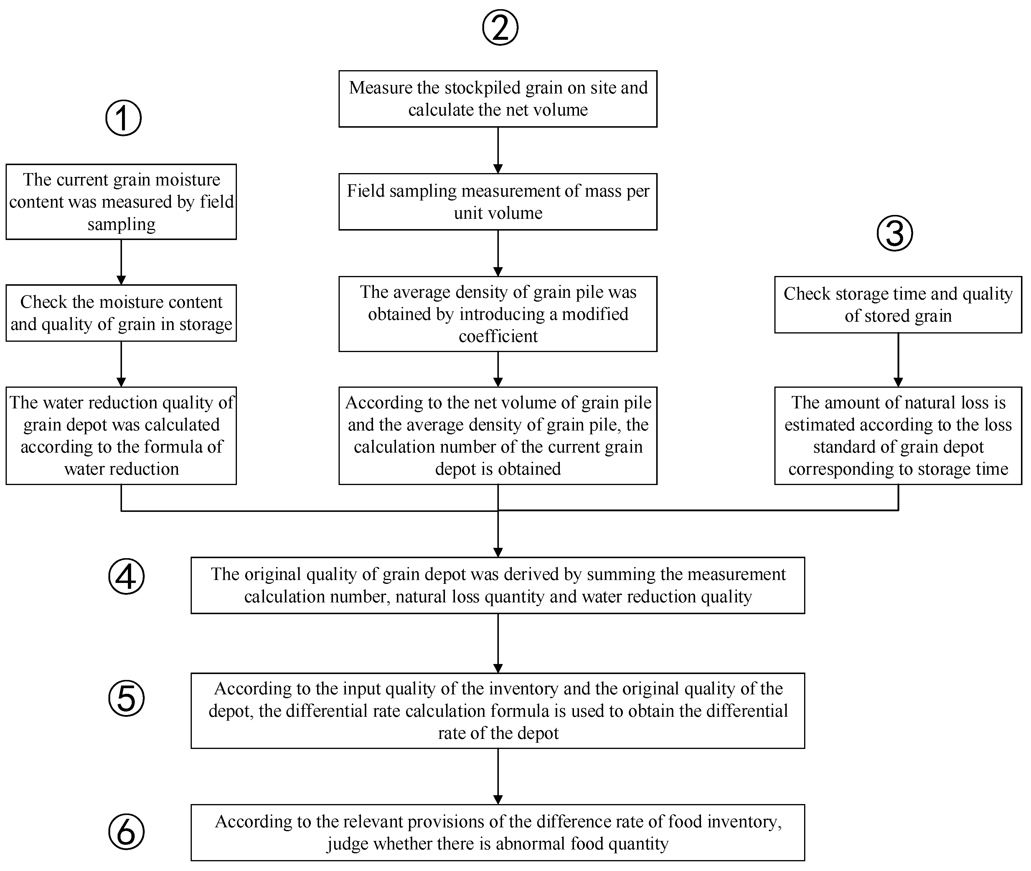
The current commonly used grain quantity inspection method in Chinese warehouse clearance is shown in Figure 1. The specific implementation steps are as follows:

Step 1: Measure the water content of the current grain through on-site sampling, check the water content of the grain in the storage and the total mass of the grain in the storage, and calculate the grain quality reduced by water reduction using Formula (1).

Step 2: Measure the volume of the grain storage pile on site, and calculate the net volume of the grain pile by subtracting the volume from Formula (2). The measured volume of the grain pile is the volume of the grain pile obtained by the laser or image measurement and inspection equipment of the grain depot, and the deducted volume is the volume protruding from the bottom or side surface of the grain depot (including infrastructure facilities such as floor cages). The average density of grain depot is obtained by introducing Formula (3) for calculating the unit volume mass through field sampling, and the calculation number for measuring the current grain depot is obtained by multiplying the net volume of the grain depot and the average density of the grain depot, as shown in Formula (4).

Step 3: Check the grain storage time and the book quality of stored grain, and establish the loss calculation Formula (5) to estimate the amount of natural loss according to the grain storage loss standard corresponding to the storage time.

Step 4: According to the measurement calculation number, the amount of natural loss, and the quality of water reduction, calculate the original quality of the grain depot (measured quality) by using Formula (6). The final grain quantity is obtained using Formula (7).

Step 5: According to the input quality of the inventory and the original quality of the grain depot, the error rate calculation Formula (8) is used to obtain the error rate of the grain depot.

Step 6: Determine if there is an anomalous amount of grain in the stock in accordance with the relevant regulations on the control of the differential rate of grain in the stock.

The formula for calculating the loss of moisture from the mass of a grain stock is as follows:

$$W_1=W({\sigma }_1-{\sigma }_2)/(100-{\sigma }_2)$$

(1)

where $W_1$ is the actual book mass of the grain in storage, $W$ is the actual book mass of the grain in storage, ${\sigma }_1$ is the moisture content of the grain in storage, and ${\sigma }_2$ is the measured moisture content.

The formula used to calculate the net volume of the grain pile is as follows:

$$V=V_1-V_2$$

(2)

where V is the net pile volume, $V_1$ is the measured pile volume, and $V_2$ is the volume to be subtracted.

The average density of the grain pile compensated by the introduction of the correction factor is as follows:

$$\rho ={k\rho }_1$$

(3)

where $\rho$ is the average density of the grain pile, ${\rho }_1$ is the measured volume weight, and $k$ is the correction factor, which is set according to the numerical relation between the stored volume weight and the measured volume weight.

Currently, the formula for calculating grain quantity widely used in the process of grain depot inspection is as follows:

$$W_2=\rho V$$

(4)

where $W_2$ is the grain quality obtained by using the average density of the grain pile after modified calculation.

According to China’s national standard for the physical inspection of grain stocks, natural storage loss rate for different storage years should be as follows: no more than 0.1 percent within six months, no more than 0.15 percent within six months, and no more than 0.2 percent within one year. According to the above criteria, the formula for calculating the amount of natural loss in grain depots is as follows:

$$W_3=\mu W$$

(5)

where $W_3$ is the natural loss mass of the grain, $\mu$ is the natural loss coefficient, and $W_1$ is the actual book mass of the grain put into storage.

Accordingly, the formula for calculating the original quality of the grain depot can be calculated as follows:

$$W_4=W_1+W_2{+W}_3$$

(6)

The formula for the measured grain pile mass, also known as the empirical formula, is computed as follows:

$$W_4=W{(\sigma }_1-{\sigma }_2)/(100-{\sigma }_2)+{k\rho }_1(V_1-V_2)+\mu W$$

(7)

The grain quality error rate for grain depots is calculated as follows:

$$\gamma =(W-W_4)/W$$

(8)

where $\gamma$ is the difference rate under percentage conversion.

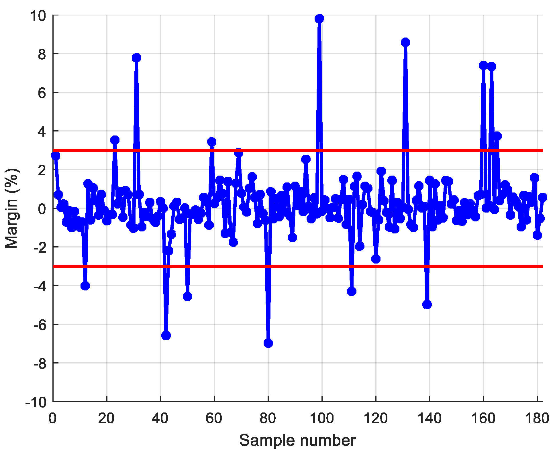
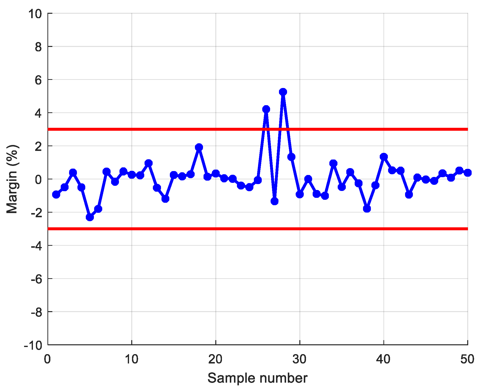
In the process of the actual grain quantity inspection, according to China’s “Food and Material Reserve Law Enforcement Supervision Work Regulations”, if the standard bulk grain difference rate is within ±2% and the non-standard grain difference rate is within ±3%, it is determined that the account is consistent. Otherwise, it is determined that there is a grain deviation, but it is also necessary to analyze the storage quality, incomplete grain, storage month, and other aspects of the stored grain in order to determine if there is a grain quantity problem. Thus, the regular grain count calculation is the basis for the grain count check.

2.2. The Selection of Correction Factors

Through the analysis of Formula (4), it can be seen that the calculation method of grain density correction coefficient is very important. Grain depot managers have accumulated experience and suggest that the correction coefficient usually falls within the range of 1.01 to 1.08. However, it is important to consider the actual storage conditions and their impact on the average density of the grain pile. These factors also play a role in determining the appropriate correction coefficient. When selecting the correction coefficient, the grain depot management department takes into account several principles. Firstly, since grains with higher quality grades have a fuller and more tightly packed internal structure, a slightly larger correction coefficient is chosen. Secondly, as the grain storage time increases, the internal grain pile becomes denser, warranting a slightly larger correction coefficient. Thirdly, the correction coefficient is larger for higher grain loads compared to that of lower grain loads. Fourthly, manual warehousing requires a larger correction coefficient than mechanical warehousing. Fifthly, in granaries located near roads, railways, airports, and large vibration sources, the grain gradually compresses due to the impact of vibrations, resulting in a larger correction coefficient. Lastly, the more ventilation cycles in the grain depot, the greater the correction factor. Although the above rules on the selection of the grain pile correction coefficient can improve the accuracy of grain quantity detection in the grain depot to a certain extent, this method is greatly affected by human factors and cannot meet the needs of grain quantity inspection in the grain depot.

3. Principle of SVR Prediction Model

3.1. Principle of Algorithm Design

The SVR prediction model is an SVM based on the introduction of the insensitive loss error function $\epsilon$. By finding an optimal classification surface, the error of all training samples from the optimal classification surface is minimized to solve the regression fitting problem of the SVM [33,34].

The principle of the SVR prediction model is as follows:

Assume that the given sample is $\left\{{(x}_{\mathrm{I}},y_i),i=\mathrm{1,2},\dots ,m\right\}$, $x_i\in R^n$, $y_i\in R^n$, where $m$ is the number of samples and $n$ is the sample dimension. Correspondingly, the regression function constructed in the high-dimensional feature space is as follows:

$$f\left(x\right)=w\Phi \left(x\right)+b$$

(9)

where $\Phi \left(x\right)$ is the nonlinear mapping function from $R^{\mathrm{n}}$ to the higher dimensional eigenspace; $w$ is the weight vector of the hyperplane; and $b$ indicates bias.

By definition, the linear insensitive loss error function $\mathsf{\epsilon }$ is as follows:

$$L\left(f\left(x\right),y,\epsilon \right)=\left\{\begin{array}{c}0, \left|y-f\left(x\right)\right|\le \epsilon \\ \left|y-f\left(x\right)\right|-\epsilon , \left|y-f\left(x\right)\right|>\epsilon \end{array}\right.$$

(10)

where $f\left(x\right)$ is the predicted value returned by the regression function, and $\mathrm{y}$ is the corresponding true value. If the difference between $f\left(x\right)$ and $y$ is less than or equal to $\epsilon$, the loss is judged to be 0.

According to the principle of structural risk minimization [8] and the introduction of relaxation variables ${\xi }_{\mathrm{i}}$ and ${\xi }_{\mathrm{i}}^{\mathrm{*}}$, the problem of seeking $w$ and $b$ is transformed into the problem of solving minimum values under constraints, and the mathematical description equation set is established as follows:

$$\left\{\begin{array}{c}\begin{array}{c}\min \left[{\frac{1}{2}‖w‖}^2+C{\sum }_{i=1}^m({\xi }_i+{\xi }_i^{*})\right]\\ \mathrm{s}.\mathrm{t}.\left\{\begin{array}{c}{y}_i-\left[w\Phi \left(x_i\right)+b\right]\le \epsilon +{\xi }_i\\ \left[w\Phi \left(x_i\right)+b\right]-y_i {\le \epsilon +\xi }_i^{*}\\ {\xi }_i , {\xi }_i^{*} \ge 0,i=\mathrm{1,2},\dots ,m\end{array}\right.\end{array}\end{array}\right.$$

(11)

where $C$ is the error penalty factor. The larger the value of $C$, the larger the penalty on samples with training errors larger than $\mathsf{\epsilon }$, which limits the error requirement of the regression function. A smaller value of $C$ implies a smaller error of the regression function.

In order to solve Formula (11), the Lagrange Function is introduced and transformed into a solution problem in its dual form, which is as follows:

$$\left\{\begin{array}{c}\max \left\{-\frac{1}{2}{\sum }_{i=1}^m{\sum }_{j=1}^m\left(a_i-a_i^{*}\right)\left(a_j-a_j^{*}\right)K(x_i,x_j)-\epsilon {\sum }_{i=1}^m\left(a_i+a_i^{*}\right)+{\sum }_{i=1}^m{y}_i\left(a_i-a_i^{*}\right)\right\}\\ \mathrm{s}.\mathrm{t}.\left\{\begin{array}{c}{\sum }_{i=1}^m\left(a_i-a_i^{*}\right)=0\\ 0\le a_i\le C\\ 0\le a_i^{*}\le C\end{array}\right.\end{array}\right.$$

(12)

$$K(x_i,x_j)=\Phi \left(x_i\right)\Phi \left(x_j\right)$$

(13)

where, $a_i$, $a_i^{*}$, $a_j$, and $a_j^{*}$ are Lagrange multipliers, and $K(x_i,x_j)$ is the kernel function.

Since Formula (12) is a complex function optimization problem with linear constraints, its solution has global optimality and uniqueness.

Suppose that the optimal solution obtained from Formula (12) is $a=\left[a_1,a_2,\dots ,a_m\right]$, $a^{*}=\left[a_1^{*},a_2^{*},\dots ,a_m^{*}\right]$; the solutions $w^{*}$ and ${ b}^{*}$ can be obtained as follows:

$$w^{*}={\sum }_{i=1}^m\left(a_i-a_i^{*}\right)\Phi \left(x_i\right)$$

(14)

$$b^{*}=\frac{1}{N_{nsv}}\left\{{\sum }_{0<a_i<C}\left[y_i-{\sum }_{x_i\in SV}\left(a_i-a_i^{*}\right)K(x_i,x_j)-\epsilon \right]+{\sum }_{0<a_i<C}\left[y_i-{\sum }_{x_j\in SV}\left(a_j-a_j^{*}\right)K(x_i,x_j)+\epsilon \right]\right\}$$

(15)

where $N_{nsv}$ is the number of SVM.

The regression function $f\left(x\right)=w^{*}\Phi \left(x\right)+b^{*}$ expression can be converted to the following:

$$f(x)={\sum }_{i=1}^m\left(a_i-a_i^{*}\right)K(x_i,x_j)+b^{*}$$

(16)

Among them, only some parameters have $\left(a_i-a_i^{*}\right)\ne 0$, and their corresponding samples are the support vectors in the above problem.

3.2. Kernel Function Selection

Since different types of kernel functions and parameters have a large impact on the generalization ability of predictive models, the comparison optimization of kernel functions is necessary to ensure the prediction accuracy of SVR prediction models [35].

Common kernel functions are as follows:

The linear kernel function is

$$K(x_i,x_j)=x_i{x}_j$$

(17)

The polynomial kernel function of order $d$ is

$$K(x_i,x_j)={\left(x_i{x}_j+1\right)}^d$$

(18)

The radial basis kernel function is

$$K(x_i,x_j)=exp\left(-\frac{{‖x_j{-x}_i‖}^2}{2{\sigma }^2}\right)$$

(19)

The Sigmoid kernel with arguments $k$ and $\theta$ is

$$K(x_i,x_j)=tanh\left(k\right(x_i{x}_j)+\theta )$$

(20)

In the formula, the related parameters of $C$, $d$, $\sigma$, $k$, $\theta$, and other kernel functions involved can be selected and determined by the optimization algorithm.

3.3. Evaluation Indicators

To objectively evaluate the effectiveness of SVR predictions, two metrics, the mean squared error E and the coefficient of determination $R^2$, are used to evaluate the performance of SVR prediction models [36,37]. The smaller the mean squared error E, the better the performance of the SVR prediction model. The coefficient of determination is in the range of [0,1], and the closer $R^2$ is to the value 1, the better the SVR prediction model. Otherwise, the performance of SVR prediction model is worse. If the resulting SVR regression model does not satisfy the set requirement, the SVR regression model is reconstructed by modifying the model parameters or changing the kernel function type until the set requirement is satisfied. The mean square error E and the coefficient of determination $R^2$ to be determined are calculated as follows:

$$E=\frac{1}{m}{\sum }_{i=1}^m{\left({\widehat{y}}_i-y_i\right)}^2$$

(21)

$$R^2=\frac{{\left(\mathrm{m}{\sum }_{\mathrm{i}=1}^{\mathrm{m}}{\widehat{\mathrm{y}}}_{\mathrm{i}}{\mathrm{y}}_{\mathrm{i}}-{\sum }_{\mathrm{i}=1}^{\mathrm{m}}{\widehat{\mathrm{y}}}_{\mathrm{i}}{\sum }_{\mathrm{i}=1}^{\mathrm{m}}{\mathrm{y}}_{\mathrm{i}}\right)}^2}{\left(\mathrm{m}{\sum }_{\mathrm{i}=1}^{\mathrm{m}}{{\widehat{\mathrm{y}}}_{\mathrm{i}}}^2-({\sum }_{\mathrm{i}=1}^{\mathrm{m}}{{\widehat{\mathrm{y}}}_{\mathrm{i}})}^2\right)\left(\mathrm{m}{\sum }_{\mathrm{i}=1}^{\mathrm{m}}{\mathrm{y}}_{\mathrm{i}}^2-({\sum }_{\mathrm{i}=1}^{\mathrm{m}}{{\mathrm{y}}_{\mathrm{i}}^2)}^2\right)}$$

(22)

where $m$ is the number of samples in the whole test set; $y_{i }$ is the true value of the $i$ th sample; and ${\widehat{y}}_i$ is the predicted value for the i th sample.

3.4. SVR Prediction Model Algorithm Design of Grain Depot

In this study, the depot clearing and inspection steps were combined with the SVR prediction model prediction, which was used in place of the empirical formulation to eliminate the interference of human factors in the correction weight setting and the natural loss computation process. The SVR prediction model was constructed as shown in Figure 2.

First, the collection of the grain depot inventory data was sorted, the data related to the grain depot inventory were selected as samples, and a normalization process was performed to eliminate the dimensional differences of different metrics and speed up the network learning. Second, the test samples were selected from the total sample summary, the structure of the prediction model was set, the kernel function and related parameters were selected, the SVR prediction model was constructed, the evaluation index of the SVR prediction model was established, and the index was used to judge whether the model met the accuracy requirements. If this requirement was not met, the kernel and associated parameters were replaced until the accuracy requirement was met and the SVR prediction model was formed under the optimal kernel and parameter configuration. The inventory measurements or samples to be tested were then fed into the prediction model, and the predicted amount of grain store inventory was output. Finally, the difference ratio was calculated based on the predicted inventory volume and the inventory book volume to verify that the relevant provisions were satisfied.

In this study, after choosing the kernel function and considering the actual usage conditions of grain inspection devices, we found the best parameters by choosing a cross-validation method. Since the penalty factor $\mathrm{C}$ was chosen to be larger, the number of support vectors obtained was larger and the computational cost was higher. Thus, the computational time was reduced by preferentially choosing parameter combinations with smaller values of the penalty factor $C$, under the condition that the performance of the prediction model was not different.

4. Experimental Analysis

Construction of Training and Test Samples

Since the SVR prediction model has the advantage of obtaining the optimal solution in a restricted sample, it is particularly suitable for the analysis and prediction of small-sample problems. In this study, a total of 232 sets of samples were collected for model training and testing. We randomly selected 182 samples as training samples, and the remaining 50 samples were used as test samples. A partial sample of the amount of established wheat stocks is given in

Table 1. Sample characteristics of wheat inventory data.

IMC (%)	MMC (%)	MBD (g·L−1)	ST (Month)	MNV (m3)	SBW (kg)	MW (kg)
12.3	11.6	764	29	318.019	246,422	246,108.7427
12.3	11.6	764	24	1371.176	1,113,928	1,092,281.901
12.3	11.6	764	24	192.4163	149,740	148,790.7688
12.3	11.7	764	18	4449.902	3,486,050	3,467,868.607
12.5	11.2	767	22	3783.51	2,975,000	2,956,416.531
12.4	11.9	764	21	3814.40	3,023,000	2,971,082.065
12.5	11.7	763	20	2800.38	2,237,240	2,228,516.481
12.5	11.7	763	20	679.56	537,030	540,713.7864
12.5	11.9	772	20	3776.23	3,010,000	3,004,085.459

. The sample characteristics selected in this study include the initial moisture content (IMC), the measured moisture content (MMC), the measured bulk density (MBD), the storage time (ST), the measured net volume (MNV), the storage book weight (SBW), and the empirical weight (MW).

To effectively evaluate the performance of SVR prediction models, we designed SVR prediction models based on linear kernel, radial basis kernel, and Sigmoid kernel, respectively, under the condition that other parameters were kept constant. The evaluation indexes given by Formulas (21) and (22) were used to evaluate the performance of different kernel function SVR prediction models. The smaller the mean squared error E, the better the performance of the SVR prediction model. The closer the determined coefficients were to the value 1, the better the SVR prediction model. Otherwise, the SVR prediction model performed worse. It can be seen from Figure 3 and Figure 4 that the mean square errors of the SVR prediction model based on linear kernel function and the SVR prediction model based on Sigmoid kernel function were stable and smaller, while the mean square error of the SVR prediction model based on RBF kernel function fluctuated greatly and the average value was larger. Similarly, it can be seen from Figure 5 and Figure 6 that the SVR prediction model based on the linear kernel function and the SVR prediction model based on the Sigmoid kernel function were both stable and closer to 1 than the SVR prediction model based on the RBF kernel function in terms of the evaluation of the determined coefficients. It can be seen that the SVR prediction model based on linear kernel function and the SVR prediction model based on Sigmoid kernel function were superior to the SVR prediction model based on RBF kernel function in the evaluation of the two indexes, and there was little difference between the SVR prediction model based on linear kernel function and the SVR prediction model based on Sigmoid kernel function in the rating convenience of these two indexes.

The accuracy of wheat inventory prediction is a direct evaluation of different kernel function SVR prediction models. According to China’s “Food and Material Reserve Law Enforcement Supervision Work Regulations”, an error rate within the range of 3% is considered to be a no quantity problem. As shown in Figure 7 and Figure 8, both the SVR prediction model based on the linear kernel function and the SVR prediction model based on the Sigmoid kernel function had better stability and higher accuracy than that of the SVR prediction model based on the RBF kernel function, regardless of the training and test predictions. Twenty prediction models were trained separately for testing and validation under non-kernel function conditions. The results show that the average prediction accuracy was 93.2 percent for the linear kernel, 87.4 percent for the RBF kernel, and 91 percent for the Sigmoid kernel. The best performance of the SVR prediction model based on the linear kernel function was achieved when the mean squared error, the coefficient of determination, and the rate of correct prediction were taken into account. Experiments were conducted on the construction of SVR prediction models based on linear kernel functions, and the results were predicted using the stock wheat training set, as shown in Figure 9. The predicted results for the stockpiled wheat test set are shown in Figure 10. The difference rate distribution of the 182 training samples used for training is shown in Figure 11. The marginal distributions for the 50 samples used for the test are shown in Figure 12. As can be seen from the test results, the accuracy of this test was 96 percent, which was higher than the average prediction accuracy of this model. The red line in Figure 11 and Figure 12 represents the allowable fluctuation range of the difference rate. If the predicted result fell outside the range of −3% to 3%, it indicated an abnormal quantity of grain in this grain depot.

5. Conclusions

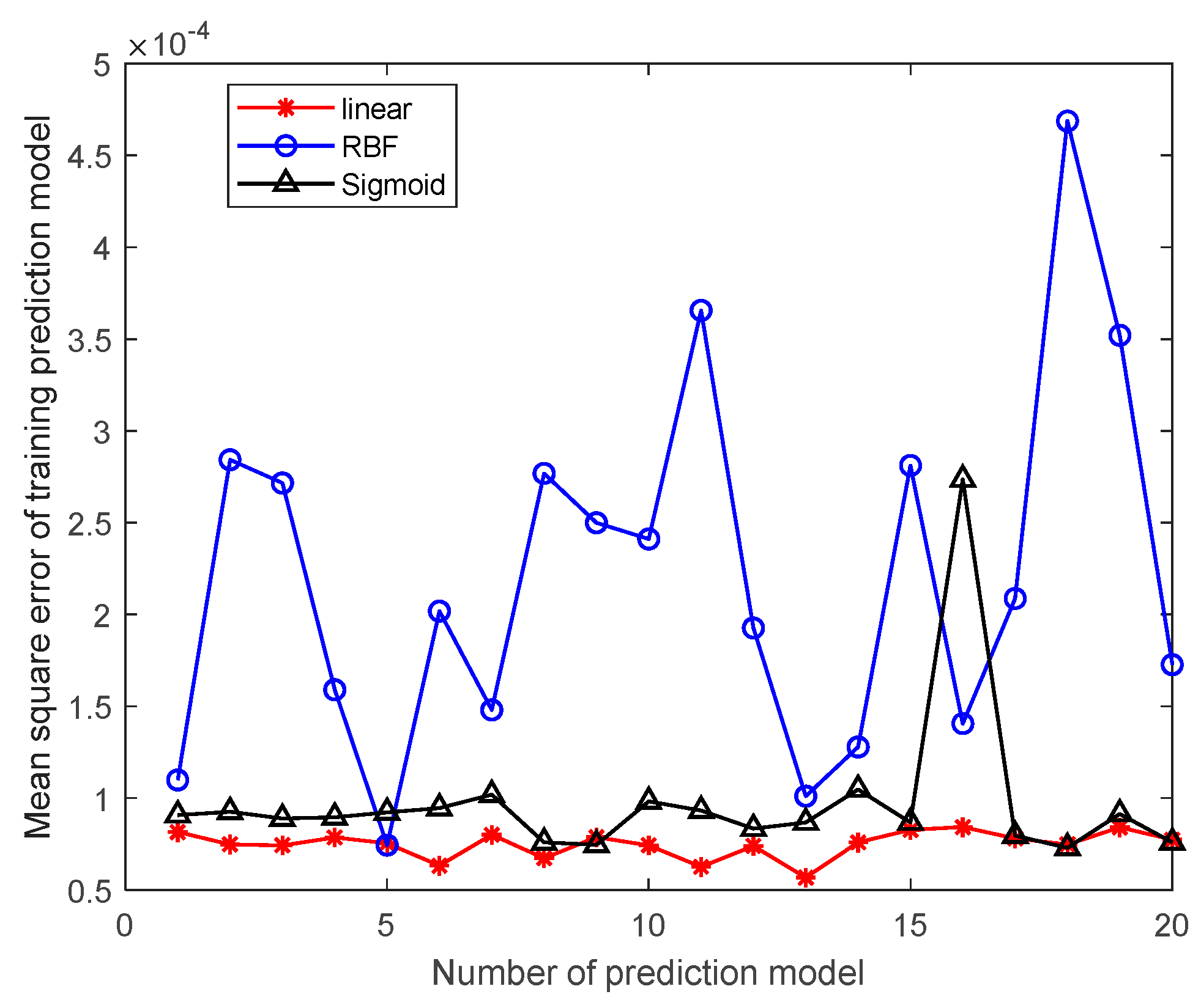
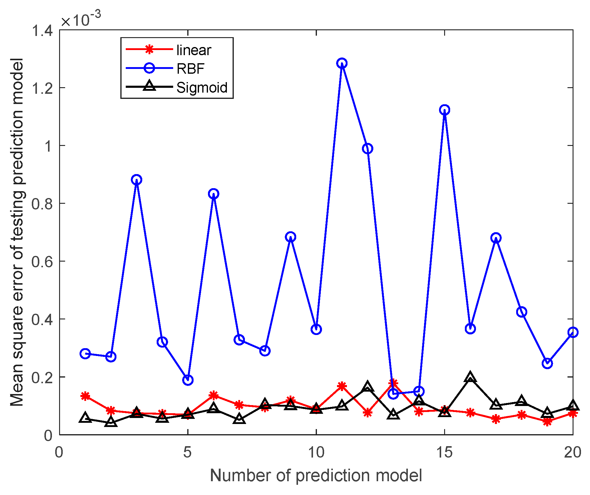
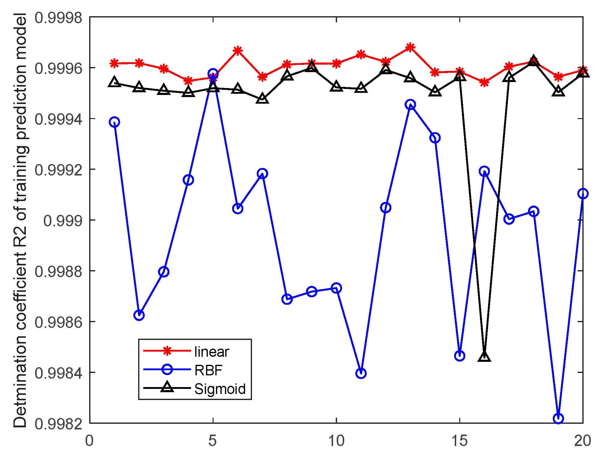
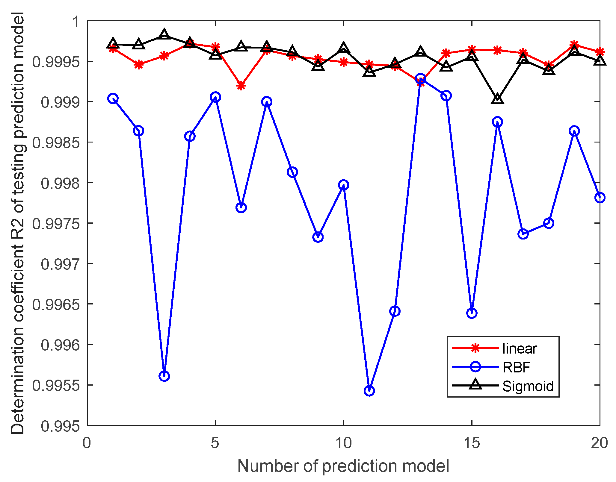
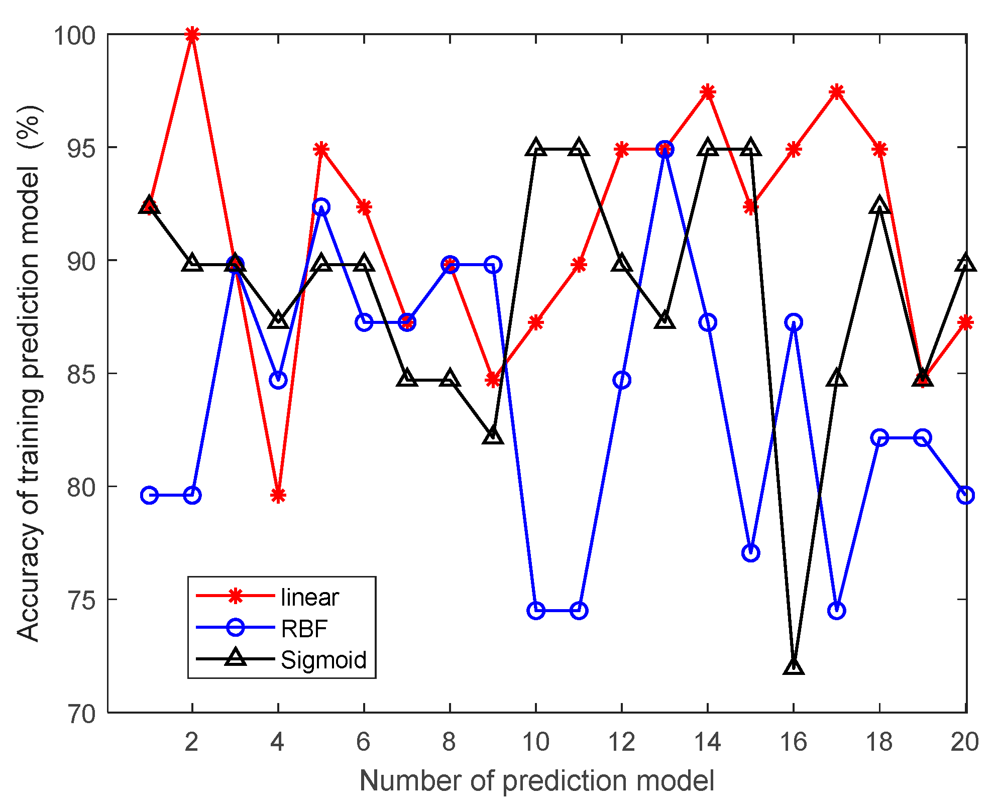
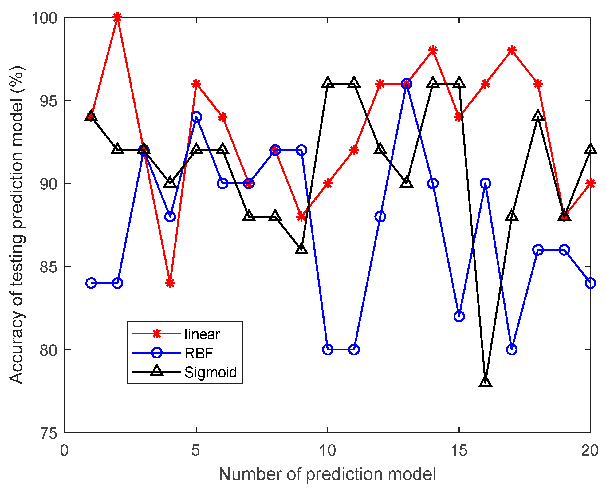
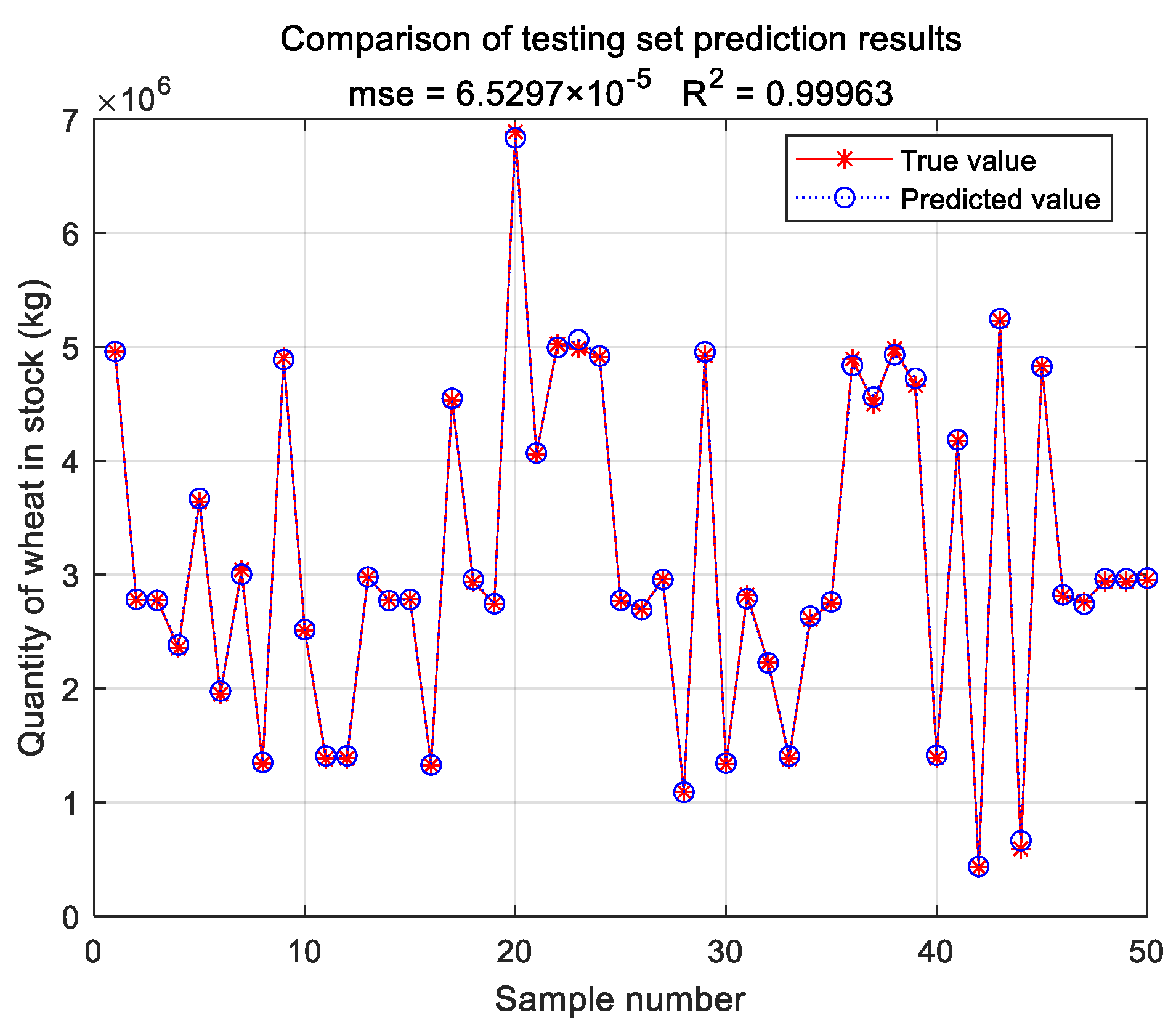
This study innovatively proposes a grain quantity monitoring method that combines wheat inventory measurement with the SVR prediction model. By learning wheat inventory information and measuring grain pile volume using a laser, combined with the trained SVR prediction model, it can greatly improve the human factor interference caused by the use of empirical formulas in the process of grain depot inspection. It improves the objectivity and accuracy of the inventory of grain depot. The model takes storage time, storage weight, storage moisture content, measured moisture content, measured bulk density, and measured net volume as training samples. Through experimental comparison, it is found that the SVR prediction model based on linear kernel function has the best prediction effect, and the average prediction accuracy of grain depot error rate reaches 93.2%.

In this study, sample selection was a complex and time-consuming task, as the accuracy of sample acquisition directly impacted the reliability of the SVR prediction model. To ensure sample accuracy, we dedicated nearly two years to collecting samples, although the number obtained remains relatively limited. Nonetheless, based on the available samples, this study proposes an SVR prediction method that combines grain storage volume measurements with the recording parameters of grain storage. This approach eliminates the issue of individuals setting the correction coefficient for average grain storage density based on experience, presenting a novel method for scientifically evaluating grain storage quantity inspection and enhancing the existing means of inspection. Therefore, only the SVR prediction method, which is suitable for small sample training, was used for this research. In future studies, we plan to collect more sample data for grain storage forecasting and expand the sample characteristics. Once we have accumulated a sufficient amount of sample data, we will explore the use of deep-learning methods to address the problem. Deep learning has unique advantages in handling large samples and complex tasks, and it can potentially provide accurate predictions for grain quantity in grain storage.