Early Fast Cost Estimates of Sewerage Projects Construction Costs Based on Ensembles of Neural Networks

Featured Application

The potential applications of the research results, particularly the models utilizing ensembles of neural networks, offer the feasibility of early cost estimates for sewerage projects. The cost estimates of construction works, derived from the developed models, can be generated based on the essential features of sewerage projects that are accessible for analysis prior to the commencement of detailed design.

Abstract

This paper presents research results on the development of an original cost prediction model for construction costs in sewerage projects. The focus is placed on fast cost estimates applicable in the early stages of a project, based on fundamental information available during the initial design phase of sanitary sewers prior to the detailed design. The originality and novelty of this research lie in the application of artificial neural network ensembles, which include a combination of several individual neural networks and the use of simple averaging and generalized averaging approaches. The research resulted in the development of two ensemble-based models, including five neural networks that were trained and tested using data collected from 125 sewerage projects completed in the Czech Republic between 2018 and 2022. The data included information relevant to various aspects of projects and contract costs, updated to account for changes in costs over time. The developed models present satisfactory predictive performance, especially the ensemble model based on simple averaging, which offers prediction accuracy within the range of ±30% (in terms of percentage errors) for over 90% of the training and testing samples. The developed models, based on the ensembles of neural networks, outperformed the benchmark model based on the classical approach and the use of multiple linear regression.

1. Introduction

Sanitary sewerage systems, as a part of built infrastructure, are unquestionably of high significance for modern societies. The role of sewer networks is to collect and transfer wastewater from buildings (residential, commercial, or industrial) and all kinds of public and private establishments to a point of treatment and disposal. These systems are the results of construction projects aiming to either build new or renovate existing sewerages. Most of such projects—one may even dare to say that the overwhelming majority—are financed from public funds.

Sewer projects, regarding their specificity, require careful analyses, design, and planning so that the technical requirements (especially flow capacity) are met. When planning is concerned, cost analyses are of key importance as completion of a project within a budget is one of the “hard” goals and key measures of any construction project success. Thus, there is a need for realistic cost predictions, analyses, and estimates, which make the goal achievable. These predictions should reflect the progress of the design process and available information, which evolves from basic and fundamental to definite and accurate. The estimates that play a specific role are called early estimates. These rely on basic information and some essential parameters of a project and are provided in the early stage of the design process. On the one hand, the expected accuracy is low; on the other hand, this is when the impact on the construction cost is great, as the essential choices and decisions for the project are made.

In the construction industry, cost estimates play a pivotal role in project planning and execution. These estimates provide a closely approximated assessment of expected expenses, empowering project stakeholders to make well-informed decisions. The accuracy of cost estimates holds paramount importance in activities such as budgeting, securing financial resources, and ensuring the successful completion of construction projects. The precision of cost estimates can vary, spanning from rough order of magnitude estimates at the project’s conceptual inception to highly detailed assessments during the design and pre-construction phases. These estimates undergo continual refinement as additional project-specific information becomes available. It is imperative to acknowledge that erroneous cost estimates can result in budget overruns, project delays, and disputes within the construction process. Hence, the development of precise, well-informed cost estimates emerges as a critical factor for the effective and economically viable execution of construction projects.

Advances and progress in data sciences and artificial intelligence tools for processing information—especially for prediction problems—opened possibilities for the development of cost estimation methods based on the use of collected data, learning from experience, and knowledge generalization. Specifically, artificial neural networks (ANN) are tools that have significant capabilities that make them useful for early construction cost estimation; however, they are hardly reported in the literature to be applied in the case of sewerage projects.

The aim of this work is to introduce a method and model of estimating construction costs for sewerage projects based on a specific artificial intelligence tool—namely ensembles of neural networks (later referred to as EoNN). The objective of the research, the results of which are presented herein, was to develop a model capable of predicting construction costs in the early stage of a sewerage project with satisfactory accuracy.

For the purpose of model development, numerous sewerage construction projects involving the construction of new sections or the renovation of existing parts of the external gravity sewage network completed in the Czech Republic between 2018 and 2022 were analyzed. These projects served as a source of data for training artificial intelligence tools.

The paper’s content includes concise literature and state-of-the-art review; a presentation of the research assumptions, data, and methods applied for the development of the fast cost estimation model; introduction of the model itself along with the results of the research; discussion of results along with comparison with a linear regression model as a benchmark; summary and conclusions.

2. Literature Review

2.1. Sewerage Construction Projects Management

When considering sewerage construction projects, management problems become subjects of research and study, similar to other types of construction projects. Some noteworthy examples of general problems presented in the literature include the following: an optimization model for sewage rehabilitation aiming to achieve maximum effectiveness at the lowest cost, utilizing genetic algorithms [1]; a methodology for selecting and prioritizing sewerage projects within available funds and system capacity, based on dynamic programming principles [2]; a study on the risk of cost overruns in water and sewerage system construction projects [3]; the development of a new method to enhance the accuracy of Monte Carlo simulations and its validation in predicting the success likelihood of sewerage build–operate–transfer projects, based on eight case studies [4]; research on culturally appropriate organization of projects implemented through public–private partnerships [5]; theoretical and empirical analysis of issues arising in public–private partnership projects within the sewerage sector [6]; and an investigation into delay factors in sewerage projects using simulations and a dynamic systems approach [7].

Cost-related challenges within sewerage projects constitute a distinct area of focus in the research literature. In one study [8], sewerage project cost estimates are examined using two alternative approaches. The first approach integrates component cost ranges and probability values established by a panel of estimators. In contrast, the second approach involves simulating costs based on random numbers, where component values are selected randomly within specified ranges. The study [9] introduces a model that relies on the utilization of prior information for the estimation of operational costs within sewerage systems. Specifically, the authors delve into the process of modeling prior information to furnish preliminary assessments of investment requirements. To facilitate subsequent estimation, the Bayes linear estimator was employed. Another research endeavor [10] centers on the intricacies of cost comparison in wastewater treatment. The authors delve into equitable methods for comparing and allocating costs in municipal sewage treatment concerning their structure and origin. Another study [11] conducts an in-depth analysis of factors responsible for variations and the resulting costs in sewerage construction projects. The work of [12] discloses research outcomes on benchmarking sewerage systems, particularly emphasizing the analysis of investment costs. This also involves an exhaustive examination of intangible variables such as economic fluctuations and tendering strategies and how they influence construction cost calculations. A notable contribution by [13] presents an Excel-based model capable of evaluating costs associated with sewerage system environmental impact. This model comprehensively assesses investigation, investment, design, operation, maintenance, supervision, and overall annual costs. The study seeks to provide a tool to facilitate environmentally informed decisions when selecting wastewater systems. The determination of capital costs for conventional sewerage systems in developing countries is scrutinized in [14]. The analysis involves the examination of unit construction costs expressed as ranges of capital cost values. Ref. [15] presents a literature review on the lifecycle costs of complete sanitation chain systems within developing cities. Moving forward, ref. [16] conducts an analysis of time–cost models that aid in forecasting project durations of different types. The research explores how construction technology influences the relationship between time and cost, particularly focusing on trenchless and open-cut technologies. In the realm of public–private partnership sewerage projects, ref. [17] delves into transaction costs. The study employs an exploratory multi-case study method to identify potential transaction costs within these projects. Lastly, ref. [18] addresses maintenance costs in sewer systems, particularly emphasizing cost estimation. The study underscores the significance of maintenance costs within the lifecycle of construction projects and proposes a linear regression model to facilitate sewer system maintenance cost estimation.

The range of problems presented above confirms that the costs and cost management of sewerage construction projects are of significant interest and importance from a research standpoint.

2.2. Cost-Estimating Models for Sewerage Construction Projects

In the context of the focus of this paper, the most crucial aspects are the attempts to develop models that assist in estimating construction costs for sewerage projects. The early work [19] investigated the application of nonlinear regression for sewer cost modeling. The study focused on estimating the empirical parameters within separable and generalized cost functions. To model the sewer cost function, the applied technique required the optimization of the values of the nonlinear parameters. The two types of analyzed nonlinear parametric cost models are reported to exhibit relative insensitivity to minor errors in the estimated values of their model parameters. The development of cost functions for open-cut and jacking methods in sanitary sewer system construction is the subject of another work [20]. The research resulted in the formulation of cost functions applicable to open-cut and jacking methods, which are construction techniques for sewer systems. These cost functions were derived using linear regression and expressed as functions of pipe size and excavation depth. The derived functions were validated using data from several actual sewer system construction projects to verify the accuracy of cost predictions. Another work [21] presents nonlinear unit cost functions for estimating costs associated with elements of waterborne sewer infrastructure, including gravity pipes, rising mains, pump stations, and wastewater treatment facilities. As a result, a model that combines several cost functions was developed to predict the unit cost of various sewer elements. Modeling the costs related to sewer systems has also been explored in the study [22]. The approach outlined in this research relies on the utilization of multiple linear regression techniques. The authors devised and validated cost functions that pertain to various components of sewer systems, including gravity and rising pipes, manholes, and pumping stations. The costs are delineated as functions of the principal physical attributes of these components. The process of estimating the cost functions involved the application of multiple linear regression analysis. In another work [23], a parametric approach for modeling the construction costs of sewer systems is presented. The authors aimed to establish an initial cost model on a municipal level, with population size serving as the primary variable for the cost functions. By maintaining population size as an independent factor, an empirical correlation has been deduced between population size and the expenses associated with sewerage systems. Various forms of cost functions were experimented with, encompassing both linear and nonlinear formulations. The matter of early cost estimates for sewerage lines is also present in [24]. The authors employed regression analysis to formulate models for predicting early-stage costs. The study devised models grounded in linear regression, featuring the technical attributes of sewerage lines as independent variables and the estimated costs as the dependent variable.

It can be observed that several works are based on an approach in which the form of the cost function is assumed ex-ante. Both linear and nonlinear functions have been employed to model the costs of sewer systems; however, linear regression appears to be the most popular tool among researchers. Nonetheless, there are works that present attempts to employ artificial neural networks for the purpose of cost estimates in sewerage projects. In [25], a neural network is utilized as the cornerstone of a cost-estimating model designed for a budget estimation system focused on repair and/or replacement costs of sewer and water projects. The model incorporates 23 project-related factors, derived through Pareto analysis, as input variables (independent variables), while the budget estimate serves as the output (dependent variable). The authors emphasize that the proposed model not only saves time but also enhances the precision of estimates, offering clients a means to compare cost alternatives and facilitating decision-making processes in cases involving the rehabilitation of sewer and water systems. Similar work [26] deals with the problems of conceptual cost estimating for water supply and sewerage projects. This paper presents a backpropagation neural network-based model that is supposed to assist municipal authorities in the development of more accurate cost estimates for their water supply and sewer projects. Cost predictors, representing project technical parameters and serving as the model’s input, were identified on the basis of contractors’ bids analysis and covered 80% of construction work costs. The benefits of the presented model include but are not limited to, better utilization of financial resources, the provision of decision-making guidelines, and the ability to compare alternatives. Additionally, the authors claim that the model fulfills the needs of funding entities for more accurate cost estimates.

In comparison to the parametric approach, modeling costs using neural networks eliminates the need for assumptions about the equation that binds the independent variables of the models to the cost, which serves as the dependent variable.

2.3. Applications of Neural Networks and Ensembles of Neural Networks for Construction Management Problems and Cost Estimation in Construction

Artificial neural networks (ANN) are a subset of artificial intelligence tools inspired by the learning and knowledge storage patterns observed in neurobiology. They can be employed to address various classification or regression challenges. The concept and theory of neural networks have been extensively discussed in numerous works [27,28,29,30]. Neural networks possess the capacity to process data with the aim of uncovering concealed patterns. The procedure of data processing to acquire knowledge, referred to as training, is executed through specific algorithms. Following the training phase, these networks are anticipated to possess the ability to generate predictions for novel data that were not utilized in the training process. The ability to generalize knowledge is a key attribute of artificial neural networks, rendering them valuable for a range of engineering problems.

Particularly, ANN has found application in addressing cost-related challenges within the construction sector. An exemplary illustration of this is a fuzzy neural network model aimed at aiding contractors in estimating and selecting a suitable markup [31]. Investigative efforts in other work [32] centered on the evaluation of multilayer perceptron and general regression neural networks for their potential in early cost estimation for road tunnel projects. In [33], the outcomes from the utilization of general regression neural networks to predict maintenance costs associated with construction equipment are shared. Another work [34] delved into the utilization of multilayer perceptron neural networks to estimate building construction costs during the initial design phase. In [35], research results on optimizing both the cost and timeline of construction projects through the implementation of neural networks are introduced. A hybrid approach, combining multivariate regression and multilayer perceptron neural networks, was employed in another research [36] to estimate capital costs for earthmoving, loading, and unloading equipment. There are also some interesting works that explore the utilization of ANN and machine learning in the analysis of wind speed and wind direction [37,38], settlement prediction [39], and the assessment of their impact on existing structures, that is, bridges and metro, respectively.

Ensembles (also called committees) of neural networks (EoNN) have their origins in the realm of ensemble learning systems. The foundational principles of this approach can be traced back to earlier referenced works that comprehensively delve into neural network concepts [28,30], as well as works dedicated to the study of ensembles [40]. EoNN consists of individual trained artificial neural networks (ANN), each providing predictions that are subsequently aggregated, with the aim of reducing errors in comparison to standalone neural networks. The utilization of neural network ensembles within classification and regression models, as opposed to employing standalone neural networks, is anticipated to yield enhanced performance and precision [41].

Engineering applications that utilize EoNN encompass a range of engineering challenges. Some noteworthy examples include predicting the performance of substantial construction equipment, specifically tunnel boring machines [42], day-ahead electricity load forecasting for buildings [43], or forecasting heating energy consumption [44]. In the context of structural engineering, ensemble models are reported to be used for predicting high-performance concrete compressive strength [45] and identifying structural damage [46]. Finally, an example of an EoNN application for risk analysis in the maintainability of high-rise buildings in specific tropical conditions [47] can be provided.

Due to the distinctive capabilities and advantages of EoNN, their exploration within the domain of construction cost analysis is increasingly reported for different types of projects. Attempts at developing models capable of aiding various cost analyses using an ensemble approach have been reported in recent years. In the study [48], the development of a model to assist in predicting project cost and schedule success by utilizing early planning status as inputs is presented. The results obtained validate that the proposed artificial intelligence models yield satisfactory predictive outcomes. Another publication [49] explores the application of EoNN for Macro BIM cost estimates. This research develops estimation models for the structural frames of building floors, demonstrating satisfactory accuracy. Authors of [50] center their attention on cost prediction for a specific category of objects—sports fields. The construction cost forecasting model based on EoNN is proven to outperform linear regression and models relying on single neural networks. Furthermore, an analysis of estimate errors and accuracy establishes the applicability of the proposed model in the early stages of construction projects. In [51], the text delves into predicting the construction costs of buildings’ structural elements with the use of artificial intelligence tools. The introduced models are, among others, based on multiple artificial neural networks combined into an ensemble. The EoNN-based models meet expectations for knowledge generalization and the accurate prediction of buildings’ structural frames. Furthermore, an ensemble algorithm application [52] is also employed to predict the cost of highway construction projects. The study presents a model that employs artificial intelligence tools—neural networks included—in a stacking ensemble model for cost prediction.

2.4. Literature Review Summary

A literature review allows for a justifiable assumption that EoNN, when applied as the core of a construction cost estimation model for a specific type of construction object, will yield better results compared to models based on linear regression or single neural networks. On the other hand, works reporting the application of EoNN for predicting construction costs in the context of sewerage projects have not been found thus far. This paper aims to address this gap.

3. Methodology

Regarding public works tenders, the investor is required to disclose the expected value of the contract [53]. Additionally, information about the approximate value of the sewerage project is crucial during the design phase to select the optimal solution, not only from a technical standpoint but also from an economic perspective. Estimating the value of construction works poses a significant challenge, particularly when detailed project documentation is unavailable and only basic data and parameters are known. These estimates are typically provided by cost engineers and often rely on the use of technical–economic indicators, which may result in significantly inaccurate estimates [54]. The starting point of the research was the idea of a cost prediction model capable of providing estimates for sewerage construction projects utilizing information about the project available in the early design phase.

The following note aims to provide a concise overview of the broader context of the research. The construction industry in the Czech Republic is a vital sector of the country’s economy, contributing to infrastructure development, residential and commercial building projects, and employment opportunities. The industry has witnessed steady growth and modernization in recent years. The construction sector plays a significant role in the country’s economy. It contributes to GDP and provides jobs for a considerable portion of the workforce. In the context of the research presented herein, it is worth mentioning that infrastructure development, which encompasses sewerage construction projects, in the Czech Republic reflects the broader European trend of modernization, sustainable development, and ecology. It continues to play a pivotal role in the country’s development. In the Czech Republic, the percentage of the population supplied with water from the public water supply reached 94.6% in 2020. In the case of connection to the sewage system, this percentage reached a value of 86.1% [55]. Although this figure may appear satisfactory, in reality, sewerage systems are readily available in larger agglomerations, and significant gaps exist in smaller settlements. It is worth noting that construction works related to sewers encompass not only the renovation of old networks and the establishment of new networks for new buildings but also the expansion of sewerage systems in already existing built-up areas.

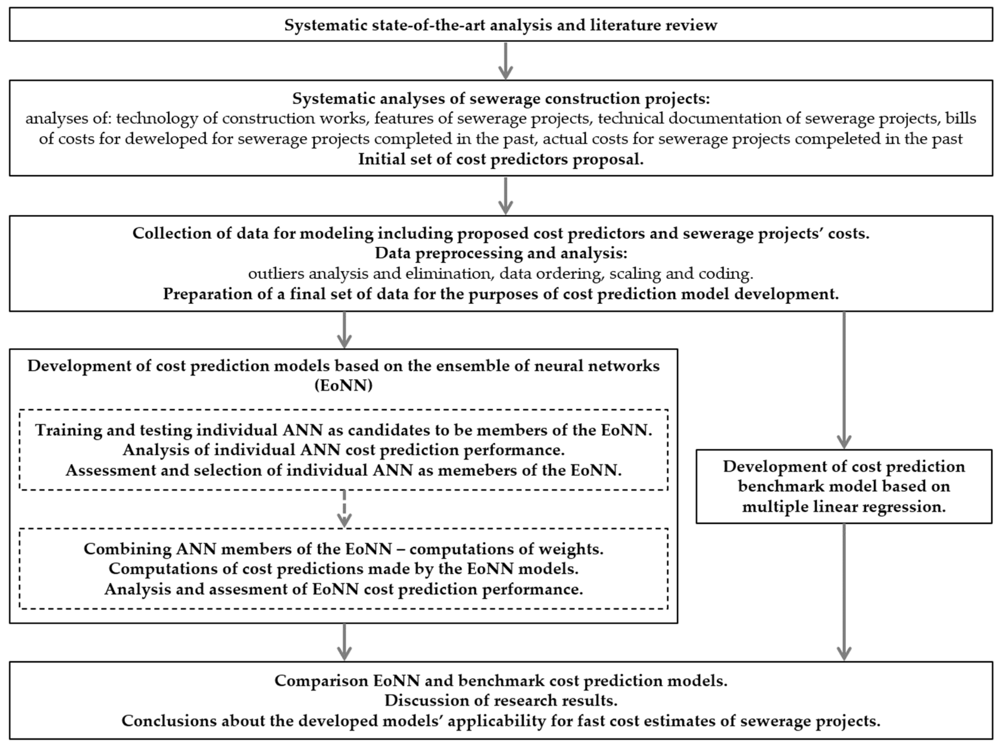
The research’s general ideogram is depicted in Figure 1, illustrating the successive steps taken by the authors.

On the basis of the steps covering the state-of-the-art and literature review, as well as analyses of sewerage construction projects completed in the Czech Republic between 2018 and 2022, an initial set of cost predictors (potential independent variables serving as input for the EoNN-based model to be developed) was proposed.

As the research focused on projects aimed at constructing new sections or upgrading existing sections of external gravity sewage networks, the cost predictors were expected to reflect the specificity of such construction projects. The analyzed projects involved separated sewer systems, with wastewater and stormwater runoffs in separate pipes. (An important point to note is that the analyzed projects did not incorporate combined runoffs; that is, the runoffs for wastewater and stormwater in a single pipe). Despite the fact that wastewater systems are connected to the existing sewage treatment plant, the plants themselves were not part of the analyzed projects, and thus, no related cost predictors were considered.

The mentioned set of cost predictors is presented in

Table 1. Initial set of cost predictors.

Cost Predictor	Input Information Description	Value
Type of project	New construction or renovation	Descriptive
Sewer pipe’s length	Size of a project, complexity of a project, quantity of works	Numerical (length)
Type of sewer pipe material	Technical parameter, material parameter, applied solution	Descriptive
Sewer pipe’s diameter	Technical parameter, applied solution, capacity of a sewer	Descriptive
Average depth of trench	Technical parameter, temporary works, safety issues	Numerical (depth)
Groundwater table level	Technical parameter, ground conditions, temporary works, safety issues	Descriptive
Class of soil	Technical parameter, ground conditions parameter, safety issues	Descriptive
Number of manholes	Size of a project, complexity of a project, safety issues	Numerical (count)
Number of crossings with other services	Complexity of a project, temporary works, safety issues	Numerical (count)
Works on unpaved surface	Conditions of works, complexity of works, soil type waste production, quantity of works	Numerical (length)
Works on paved surface	Conditions of works, complexity of works, rubble type waste production, quantity of works	Numerical (length)
Debris removal distance	Conditions of works, waste management parameter	Numerical (length)

, which includes selected types of cost predictors and descriptions of the information that is supposed to be input into the model (this information is succinctly explained in the table). Moreover, the table presents raw values of cost predictors, as they were collected before pre-processing, ordering, and scaling.

In the next step, data for the purposes of the cost prediction model were collected. This step involved the analysis of technical and design documentation, quantity surveys, cost estimates, as well as public client queries for 135 sewerage projects. This provided data reflecting the raw values of cost predictors (as presented in Table 1), along with real-life contract net costs (excluding value-added tax) of sewerage project construction works.

It is noteworthy that, through the systematic analysis of sewerage construction projects (which constituted the second phase of the research), it was observed that the previously mentioned type of runoff, whether wastewater or stormwater, did not impact the costs. From both technological and construction cost perspectives, it does not matter which type of runoff is being constructed. Therefore, this information is excluded as a predictor of costs.

Due to changes in the value of money and cost variability over time, the values of contract net costs were updated for the end of the first half of the year 2023. The updated rule is provided below.

$$UCC={ACC}_t·\prod _{i=t}^n{CI}_i$$

(1)

where:

• UCC—updated contract net cost of a sewerage project;
• ACC_t—actual contract net cost of sewerage projects, which was awarded in the t-th half-year period between the beginning of 2018 and the end of 2022;
• CI_i—cost index for i-th half-year period between the beginning of 2018 and the first half of the 2023 year;
• n—stands for the first half of the 2023 year.

Cost index values that were used to update contract net costs are published periodically by a Czech company, RTS^®, a developer and provider of a price information system for the construction industry in the Czech Republic. (It is worth mentioning that there are two main pricing systems that provide various cost information for construction cost estimation practice in the Czech Republic. These are RTS^® and URS^®.) Based on the structural and material characteristics of sewerage systems, the cost indexes used for calculations were derived from the RTS^® system. More specifically, price indicators that reflect the changes in costs in sewerage construction projects between 2018 and 2023 were used. The obtained cost indexes were also compared with the second pricing system, URS^®, to verify their correctness and applicability. In the Czech Republic, this procedure is commonly used for indexing the prices of construction works between different time periods and is also permissible for the needs of court evidence.

Outlier analysis was applied to the updated values of contract net costs for sewerage project construction works. The concept and fundamentals of outlier analysis can be found in the statistical literature, such as [56,57,58]. The purpose was to eliminate data points that deviated significantly from others, essentially excluding unusual cost values from the dataset. The approach used in this study relied on the concept of the interquartile range (IQR). The IQR was calculated as the difference between the values of the third quartile (Q3) and the first quartile (Q1), representing the range of values between these quartiles: IQR = Q3 − Q1. The rule below allowed us to identify and eliminate outlying values, as well as entire records for certain project cases from the dataset:

• If the j-th value (in the j-th record in the dataset) of updated contract net costs does not belong to the range: <Q1 − 1.5·IQR; Q3 + 1.5·IQR> → eliminate the j-th record from the dataset.

The rationale for this approach, based on the authors’ prior experiences, is that outliers can be problematic when developing cost prediction models for various construction projects, facilities, and structures, as they often represent specific, high-cost projects that are sparsely represented in datasets. Such data can distort the predictive performance of a developed model.

The collected data underwent further pre-processing. Numerical values of cost predictors were linearly scaled, while descriptive values were processed differently based on their nature; they were pseudo-fuzzy scaled, coded as one-of-n values, or converted into binary values.

Detailed information and outcomes of this step are presented in Section 4.

The next stage of the research involved computations and simulations of artificial neural networks (ANN), as well as the combination of these networks to create an ensemble. The development of models based on ensembles of neural networks (EoNN) designed to predict costs involves solving regression problems. Let the dependent variable y of such models represent the construction cost for a sewerage project. Also, let the independent variables be the cost predictors, with the vector of these variables denoted as x. The EoNN-based models are expected to approximate the mapping x → y. Importantly, in the case of employing EoNN, the approximation function h is implicitly defined as follows:

$$y=h\left(\mathit{x}\right)+\epsilon$$

(2)

where ε corresponds to the prediction error. Consequently, the formal notation for predicting costs ŷ can be expressed as follows:

$$\widehat{y}=h\left(\mathit{x}\right)$$

(3)

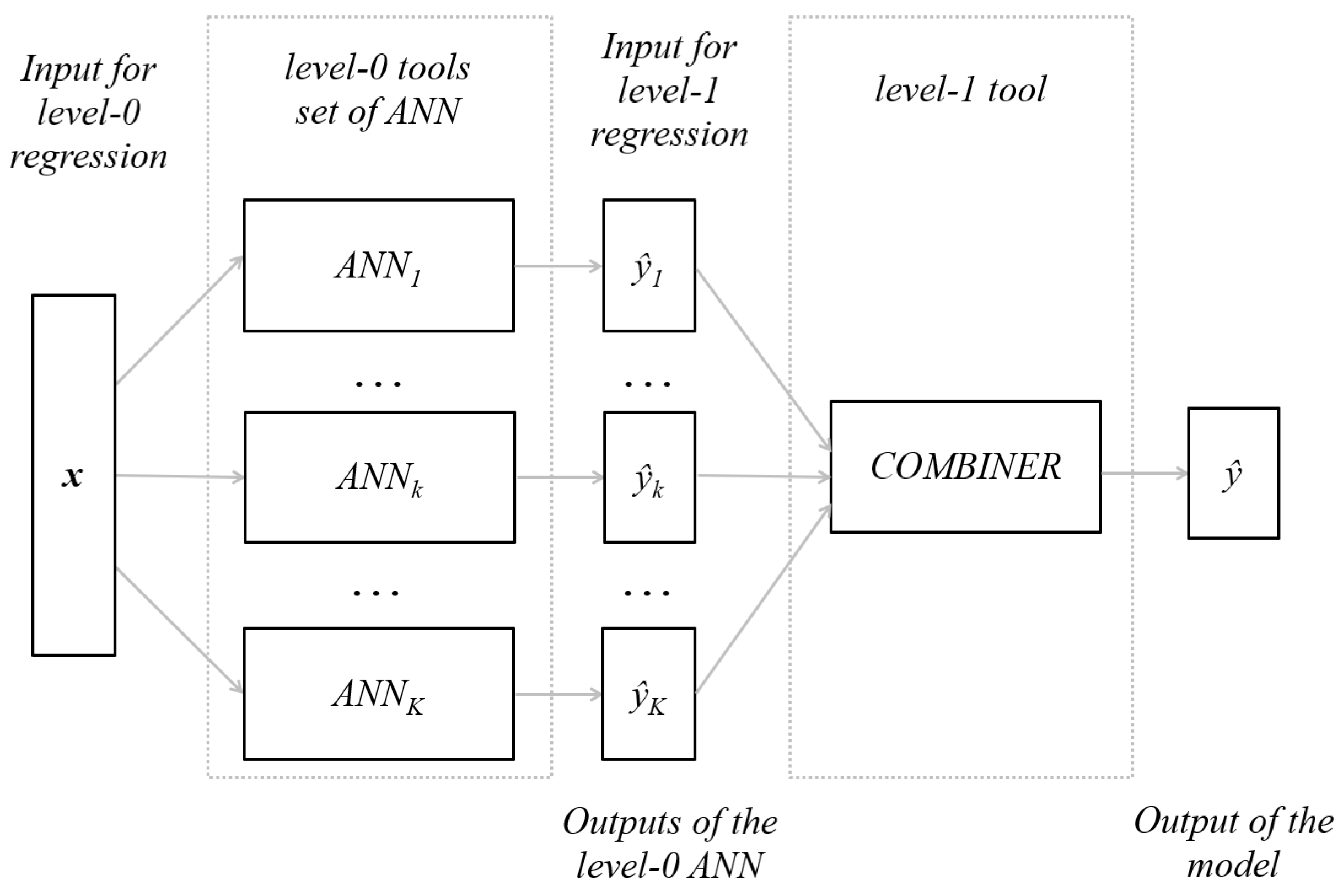
The utilization of EoNN as the core of a cost estimation model relies on combining a set of trained neural networks to form an ensemble. As outlined in [28], this set might encompass various types of networks or similar networks trained to different local minima. The two methods built on this premise, which were applied during research presented herein, are (1) ensemble averaging and (2) generalized averaging. A summary of the core principles behind the two ensemble-based methods mentioned is provided based on [28,30]. The general idea is schematically depicted in Figure 2.

At level 0, the tools consist of K experts, which are individually trained artificial neural networks (ANN), each providing cost predictions:

$${\widehat{y}}_k=f_k\left(\mathit{x}\right)$$

(4)

The cost predictions ŷ_k serve as inputs for the level-1 tool, which combines the predictions generated by the K experts to obtain a more objective final prediction of construction costs ŷ.

For ensemble averaging and generalized averaging, the combination of ŷ_k values is based on a linear combination:

$$\widehat{y}=\sum _{k=1}^K{\alpha }_k{f}_k\left(x_j\right)=\sum _{k=1}^K{\alpha }_k{\widehat{y}}_k$$

(5)

where:

• ŷ—level-1 cost prediction made by the ensemble of neural networks;
• ŷ_k—level-0 cost predictions by the k-th ANN—an expert belonging to the ensemble;
• f_k—mapping function implemented by k-th member network;
• α_k—linear combination weight for k-th expert;
• under the condition:

$$\sum _{k=1}^K{\alpha }_k=1$$

(6)

In the case of ensemble averaging, also referred to as simple averaging, the assumption is that the weights α_k are equal. In other words, cost predictions ŷ_k provided by all ensemble members equally contribute to the cost prediction of ŷ provided by the ensemble:

$${\alpha }_k=\frac{1}{K}$$

(7)

In the case of generalized averaging, the weights αk are optimized based on the training results and training errors of the ANN member networks. In this case:

$${\alpha }_k=\frac{{\sum }_{l=1}^K{\left({\mathrm{C}}^{-1}\right)}_{kl}}{{\sum }_{h=1}^K{\sum }_{l=1}^K{\left({\mathrm{C}}^{-1}\right)}_{hl}}$$

(8)

where:

• C—correlation matrix of errors produced by the members of an ensemble;
• k, h, l—are indexes of ANN member networks (used for clarity).

Matrix C elements, denoted as c_kl are computed using a finite-sample approximation:

$$c_{kl}\cong \frac{1}{N}{\sum }_p\left({\widehat{y}}_k^p-y^p\right)\left({\widehat{y}}_l^p-y^p\right)$$

(9)

where:

• p—denotes the sample for which predicted values ŷ_k and expected values ŷ;
• N—cardinality of a set of samples;
• k, l—are indexes of ANN member networks (used for clarity).

Below are the performance and error measures employed throughout the research, used for assessing both individual trained ANNs and EoNN cost predictions (R—Pearson’s correlation coefficient, ½MSE—half of mean squared error, RMSE—root mean squared error, MAPE—mean absolute percentage error, PE—percentage error).

$$R=\frac{cov(y,\widehat{y})}{{\sigma }_y{\sigma }_{\widehat{y}}}$$

(10)

$$\raisebox{1ex}{$1$}\!\left/ \!\raisebox{-1ex}{$2$}\right.MSE=\raisebox{1ex}{$1$}\!\left/ \!\raisebox{-1ex}{$2$}\right.\left(\frac{1}{M}{\sum }_p{\left(y^p-{\widehat{y}}^p\right)}^2\right)$$

(11)

$$RMSE=\sqrt{\frac{1}{M}{\sum }_p{\left(y^p-{\widehat{y}}^p\right)}^2}$$

(12)

$$MAPE=\frac{1}{M}{\sum }_p\left|\frac{y^p-{\widehat{y}}^p}{y^p}\right|$$

(13)

$$A{PE}^p=\left|\frac{y^p-{\widehat{y}}^p}{y^p}\right|·100\%$$

(14)

$${PE}^p=\frac{y^p-{\widehat{y}}^p}{y^p}·100\%$$

(15)

where:

• p—index of a sample;
• M—cardinality of subsets used in the course of the training process: for learning (subset L), validating (subset V), and testing process (subset T).
• (Division into L, V, and T subsets is explained in Section 5).

The proposed EoNN-based models are intended to assist in what are commonly known as early cost estimates for construction projects, often referred to as conceptual estimates. Based on the literature [59,60,61] and practical considerations, certain expectations regarding prediction accuracy were established. In the literature, expected accuracy for conceptual estimates typically varies, primarily between ±20% and ±30%. For the purpose of this study, it was cautiously assumed that the model’s cost predictions should not deviate by more than ±30% from actual contract costs.

The results of the development of EoNN-based models are presented in Section 5.

To assess the proposed models, benchmark models based on the linear regression approach were constructed. The comparison between the EoNN-based and benchmark models is presented, along with a discussion of the research results, in Section 6.

4. Data—Analyses and Presentation

As discussed in the previous section, data were collected for 135 sewerage construction projects. Data processing began with updates to sewerage construction costs, and Equation (1) was applied accordingly. The range of UCC values is presented in

Table 2. Values range of contract costs for sewerage projects after the update. Characteristics of updated contract cost values distribution for outliers analysis and elimination.

UCC	CZK (Thousands)	EUR 1 (Thousands)
Min	247.08	10.41
Max	44,677.63	1882.75
Range = max − min	44,430.55	1872.34
Average	3458.49	145.74
1st quartile Q1	845.02	35.61
3rd quartile Q3	3698.97	155.88
IQR	2853.96	120.27

¹ exchange rate according to the Czech National Bank for 30 June 2023 1 EUR = 23.730 CZK.

, with costs provided in both CZK and EUR currencies. The table also includes the characteristics necessary for outlier analysis and elimination, namely, Q1, Q3, and IQR values.

Following the rule for outlier analysis elimination, as discussed in Section 2, the upper and lower boundaries for the range of values were computed in CZK <−3,435,919; 7,979,909> and in EUR <−144,792; 336,279>. As the negative values of UCC were not possible, these ranges were finally adopted—in CZK <0; 7,979,909> and in EUR <0; 336,279>. UCC values exceeding the upper boundary (and, consequently, entire records in the dataset, including values of cost predictors for relevant projects) were eliminated from further processing, analyses, and model development. After the removal of outliers, the dataset consisted of 125 records.

Table 3. Descriptive statistics of updated contract cost values after outliers elimination.

UCC	CZK (Thousands)	EUR 1 (Thousands)
Min	247.08	10.41
Max	7531.92	317.40
Range = max − min	7284.85	306.99
Average	2130.52	89.78
Median	1522.22	64.14
Standard deviation	1792.95	75.56

¹ exchange rate according to the Czech National Bank for 30 June 2023 1 EUR = 23.730 CZK.

presents the descriptive statistics for UCC values after outlier elimination.

Comparing Table 2 and Table 3, it is evident that the elimination of the 10 outliers from the dataset led to a significant narrowing of the UCC value range. Consequently, high-cost projects, which were underrepresented in the dataset, were excluded from further data processing and model development. In accordance with the general assumptions for the development of the EoNN-based models, UCC is assumed to be the dependent variable, denoted later as y.

Simultaneously, the pre-processing of cost predictors, which included data analysis, ordering, scaling, and coding, was carried out. The cost predictors were assigned to the set of independent variables, denoted as x_j, as follows:

• Type of a project: x₁;
• Sewer pipe’s length: x₂;
• Type of sewer pipe material: x₃;
• Sewer pipe’s diameter: x₄;
• Average depth of trench: x₅;
• Groundwater table level: x₆;
• Class of soil: x₇;
• Number of manholes: x₈;
• Number of crossings with other services: x₉;
• Works on unpaved surface: x₁₀;
• Works on paved surface: x₁₁;
• Debris removal distance: x₁₂.

Descriptive statistics for cost predictors that originally had numerical values are presented in

Table 4. Descriptive statistics for independent variables (cost predictors) that took numerical values.

Cost Predictor	Min	Max	Range Max − Min	Average	Median	Standard Deviation
Wewer pipe’s length: x2 (m)	12	1871	1859	163.51	116.00	199.11
Average depth of trench: x5 (m)	0.58	3.68	3.10	2.41	2.41	0.55
Number of manholes: x8	0	18	18	4.63	4.00	3.50
Number of crossings with other services: x9	0	40	40	7.30	4.00	8.77
Works on unpaved surface: x10 (m)	0	1600	1600	49.79	15.00	155.07
Works on paved surface: x11 (m)	0	615	615	113.38	82.00	114.20
Debris removal distance: x12 (m)	1	30	29	11.07	5.00	11.34

. These original numerical values were linearly scaled to the range <0.1, 0.9> for the purposes of computations and computer simulations of the artificial neural network (ANN).

Data characteristics, including the original descriptive values and relevant cardinalities for cost predictors that originally had descriptive values, are presented in

Table 5. Cardinalities of values for independent variables (cost predictors) that took descriptive values, along with scaled and coded values.

Cost Predictor	Original Descriptive Value	Cardinality (Count)	Accumulated Cardinality (Count)
Type of project: x1	New construction	94	94
	Renovation	31	125
Type of sewer pipe material: x3	PE	2	2
	PVC	58	60
	PP	42	102
	Stoneware	10	112
	Glass	9	121
	Concrete	4	125
Sewer pipe’s diameter: x4	110–200 mm	5	5
	250 mm	86	91
	300 mm	17	108
	400–600 mm	13	121
	800–1000 mm	4	125
Groundwater table level: x6	Below the trench bottom level	102	102
	Above the trench bottom level	23	125
Class of soil 1: x7	I/2–I/3	28	28
	I/3	53	81
	I/3–II/4, I/3–II/5	3	84
	I/3–III/6	41	125

¹ original descriptive values according to the Czech standards.

. For the purposes of computations and computer simulations of the ANN, the original descriptive values were ordered and pseudo-fuzzy scaled into the range <0.1, 0.9>. This scaling was performed with regard to the association of the descriptive values with the costs of construction works, following the general assumption that the greater the value taken from the range, the higher the costs.

Table 6. Sample of dependent and independent variables values as prepared for computations and computer simulations of ANN.

p	y	x1	x2	x3	x4	x5	x6	x7	x8	x9	x10	x11	x12
6	335.99	0.90	0.10	0.26	0.10	0.56	0.10	0.37	0.10	0.10	0.10	0.11	0.35
14	466.37	0.10	0.13	0.26	0.30	0.44	0.10	0.90	0.19	0.10	0.12	0.15	0.13
19	534.00	0.10	0.13	0.26	0.10	0.83	0.10	0.37	0.10	0.10	0.14	0.10	0.10
25	619.74	0.10	0.11	0.42	0.30	0.65	0.10	0.10	0.19	0.16	0.10	0.15	0.90
40	842.48	0.90	0.12	0.26	0.10	0.52	0.10	0.37	0.19	0.12	0.13	0.11	0.35
47	987.58	0.90	0.12	0.74	0.50	0.38	0.90	0.37	0.19	0.22	0.12	0.14	0.35
49	1043.62	0.10	0.14	0.42	0.30	0.52	0.90	0.10	0.28	0.12	0.10	0.22	0.90
64	1642.20	0.10	0.19	0.26	0.30	0.47	0.10	0.90	0.41	0.14	0.11	0.36	0.13
76	2200.33	0.10	0.17	0.42	0.30	0.56	0.90	0.10	0.28	0.42	0.11	0.30	0.90
88	2668.12	0.90	0.14	0.74	0.50	0.42	0.10	0.37	0.14	0.58	0.11	0.23	0.21
101	3690.71	0.10	0.90	0.10	0.10	0.36	0.10	0.90	0.10	0.10	0.90	0.45	0.46
110	4515.71	0.90	0.17	0.74	0.50	0.63	0.10	0.37	0.32	0.14	0.12	0.27	0.76
119	5768.77	0.10	0.21	0.42	0.30	0.51	0.10	0.63	0.68	0.52	0.11	0.41	0.49
123	7102.82	0.10	0.29	0.26	0.30	0.81	0.90	0.37	0.59	0.78	0.11	0.67	0.16

presents a sample of the dependent variable y values alongside the scaled and coded values of independent variables x_j. The whole dataset pre-processed in such a way was utilized for further computations, computer simulations of the ANN as candidates to become the members of the ensemble, and model development.

For the purpose of model development, the entire dataset, consisting of 125 records, was divided into two main subsets. The first subset included data used for supervised training, while the second was reserved for testing.

The testing subset was carefully selected to ensure that the included records were representative of the entire dataset, equivalent to the data used during the supervised training of individual ANN candidates considered for membership in an ensemble. This testing subset, later referred to as T, comprised 15% of the data records. Data from the testing subset were not involved in the training process, as the primary aim of the testing was to assess the knowledge generalization capabilities of both individually trained ANNs and ensembles combining selected ANNs. This approach allowed for testing with data that had not been presented to the ANNs during supervised training.

The remaining 85% of the dataset was divided into two subsets for the purposes of learning, (referred to as L) and validation (referred to as V) during the supervised training of individual ANNs, which were considered candidates for ensemble membership.

The division ratio into the learning, validating, and testing subsets equaled:

L/V/T = 70%/15%/15%

The division into L and V subsets was repeated five times, resulting in five folds of data available for the supervised training of candidate ANNs. The fundamental assumption was to conduct the training process five times using different learning and validating subsets. Depending on the fold, the data records belonging to the L or V subsets were rotated between the learning and validation processes and contributed to the training process accordingly.

5. Results

According to the dataset division into five folds, as discussed in the previous section, it was assumed that the structures of the developed EoNN models would consist of five ANN multilayer perceptron networks, hereinafter referred to as MLP, each with one hidden layer.

The selection of each of the five member networks was preceded by training 100 different ANN of MLP types for each fold of L and V subsets. It was assumed that the five member networks may vary in terms of their structure or activation functions. (The general structure of the considered MLP networks was 12–H–1, including an input layer with 12 neurons reflecting the number of independent variables, a hidden layer with a varying number of neurons symbolized by H, and an output layer with 1 neuron). Possible activation functions in both the hidden and output layers included sigmoid, hyperbolic tangent, exponential, or linear functions. All networks were trained using the quick and effective Broyden–Fletcher–Goldfarb–Shanno (BFGS) algorithm.

The selection of ensemble members from the 100 candidate networks was based on the analysis of network performance. The final choice depended on the following:

• High values of the coefficient R, reflecting the correlation between the predicted and actual values of the dependent variable for learning, validating, and testing subsets;
• Close values of the ½MSE error measures computed for learning, validating, and testing subsets, denoting equivalence of the three processes;
• Analysis of MAPE and RMSE values, along with the distribution analysis of PE error measures.

The characteristics of the ANN selected to be the members of the ensemble EoNN are presented in

Table 7. Characteristics of the ANN selected to be the ensemble members.

ANN	MLP Structure	Activation Function Hidden Layer	Activation Function Output Layer	Number of Training Epochs
ANNF1	12–9–1	Exponential	Linear	22
ANNF2	12–12–1	Hyperbolic tangent	Exponential	34
ANNF3	12–12–1	Exponential	Hyperbolic tangent	15
ANNF4	12–9–1	Hyperbolic tangent	Hyperbolic tangent	42
ANNF5	12–11–1	Hyperbolic tangent	Linear	65

. (The subscripts in the table stand for the successive folds of L and V subsets—e.g., F1 for fold 1).

The five selected ANNs became EoNN members and provided level-0 predictions of UCC values, that is, updated sewerage project construction costs. Selected performance measures are presented for the EoNN members, including RMSE, MAPE, and maximum values of APE^P in

Table 8. Selected performance measures of the ANN selected to be the EoNN members.

ANN	RMSEL&V	RMSET	MAPEL&V	MAPET	max {APEPL&V}	max {APEPT}
ANNF1	453	594	19.6%	15.0%	92.1%	41.5%
ANNF2	508	521	19.2%	14.7%	80.2%	58.3%
ANNF3	533	506	22.0%	16.9%	93.9%	54.7%
ANNF4	457	391	17.6%	16.9%	67.8%	50.9%
ANNF5	402	460	15.2%	15.9%	81.5%	27.0%

.

After the selection of EoNN members, computations of the combined predictions of the entire EoNN were performed. As mentioned earlier, two variants of ensembles were considered in the course of the research:

• Model based on simple averaging—later referred to as SAV_ENS;
• Model based on generalized averaging—later referred to as GAV_ENS.

Firstly, the weights α_k were computed. For SAV_ENS, the computations based on Equation (7) were straightforward, resulting in the following:

α₁ = α₂ = α₃ = α₄ = α₅ = 0.2

For GAV_ENS, computations relied on Equations (8) and (9) and required more effort. The weights for combining outputs provided by the members of the ensemble are presented below.

α₁ = 0.109; α₂ = 0.242; α₃ = −0.185; α₄ = 0.170; α₅ = 0.664

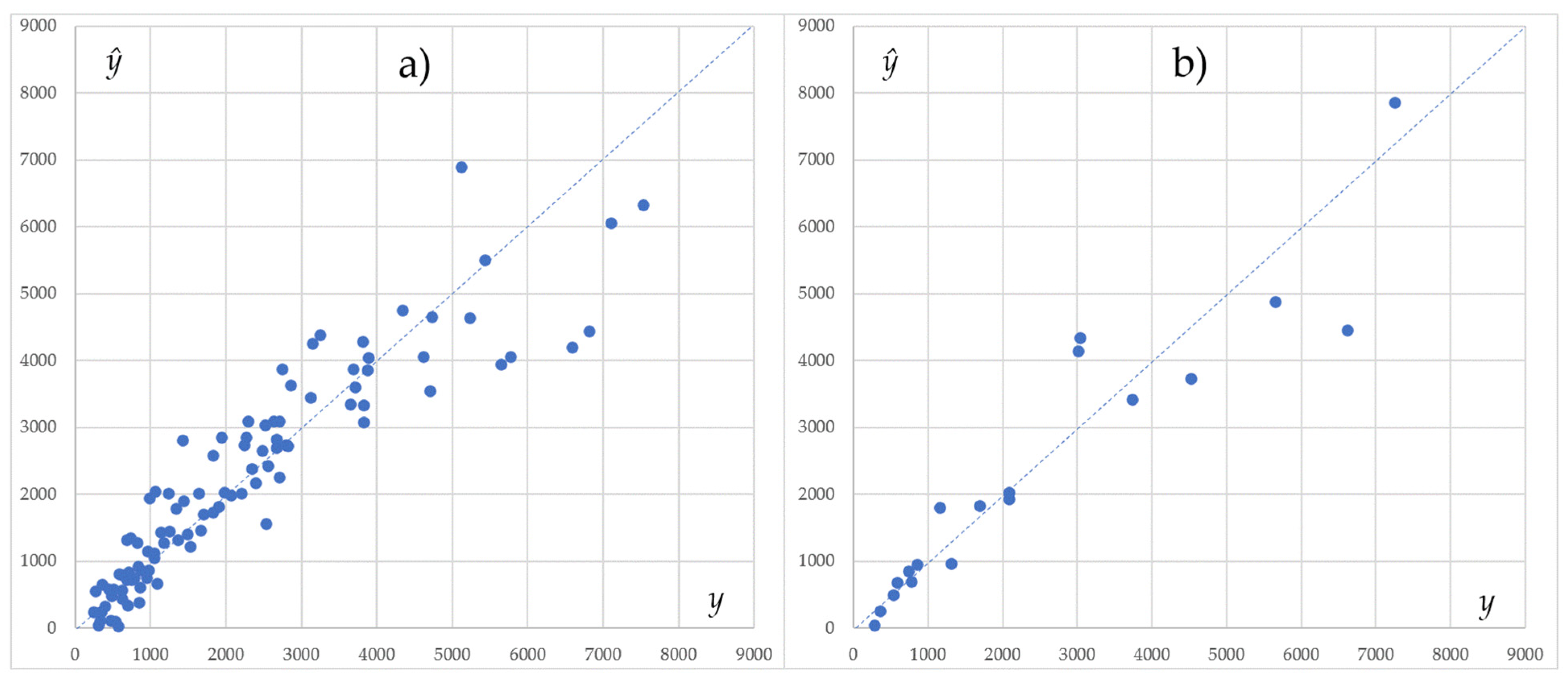
For both SAV_ENS and GAV_ENS models, further computations based on the respective weights α_k and Equation (5) were conducted to obtain level-1 predictions of sewerage project construction costs. Figure 3 and Figure 4 present scatter plots that represent real-life values of updated construction costs of sewer projects y and, on the contrary, values predicted by the developed models ŷ. Scatter plots, which are alternatively referred to as scattergrams or scatter charts, serve the purpose of providing a visual representation of data points within a two-dimensional Cartesian coordinate system. Each data point is depicted as a point or dot, facilitating the observation of the relationship between the actual values y and the predicted values ŷ. In essence, each data point on the plot corresponds to a pair of associated values. Through the utilization of scatter plots, the assessment of correlations between real-world values and values predicted by a model, as well as the evaluation of prediction quality, is carried out;

Figure 3 and Figure 4 depict results for SAV_ENS and GAV_ENS models, respectively. The points in the graphs represent the results of the training (L&V subset) and testing (T subset) processes. The distribution of points indicates that, in general, the quality of cost prediction is comparable for both ensemble-based models. There are no significant deviations, and the points are distributed along the lines of a perfect fit;

On the basis of real-life values y and values predicted by the developed models ŷ as well as Equation (10), correlation coefficients R were computed;

• For SAV_ENS: R = 0.976 for the L&V subset and R = 0.988 for T subset;
• For GAV_ENS: R = 0.972 for the L&V subset and R = 0.987 for T subset;

Correlation of y and ŷ is very high, and no significant differences between the models can be identified.

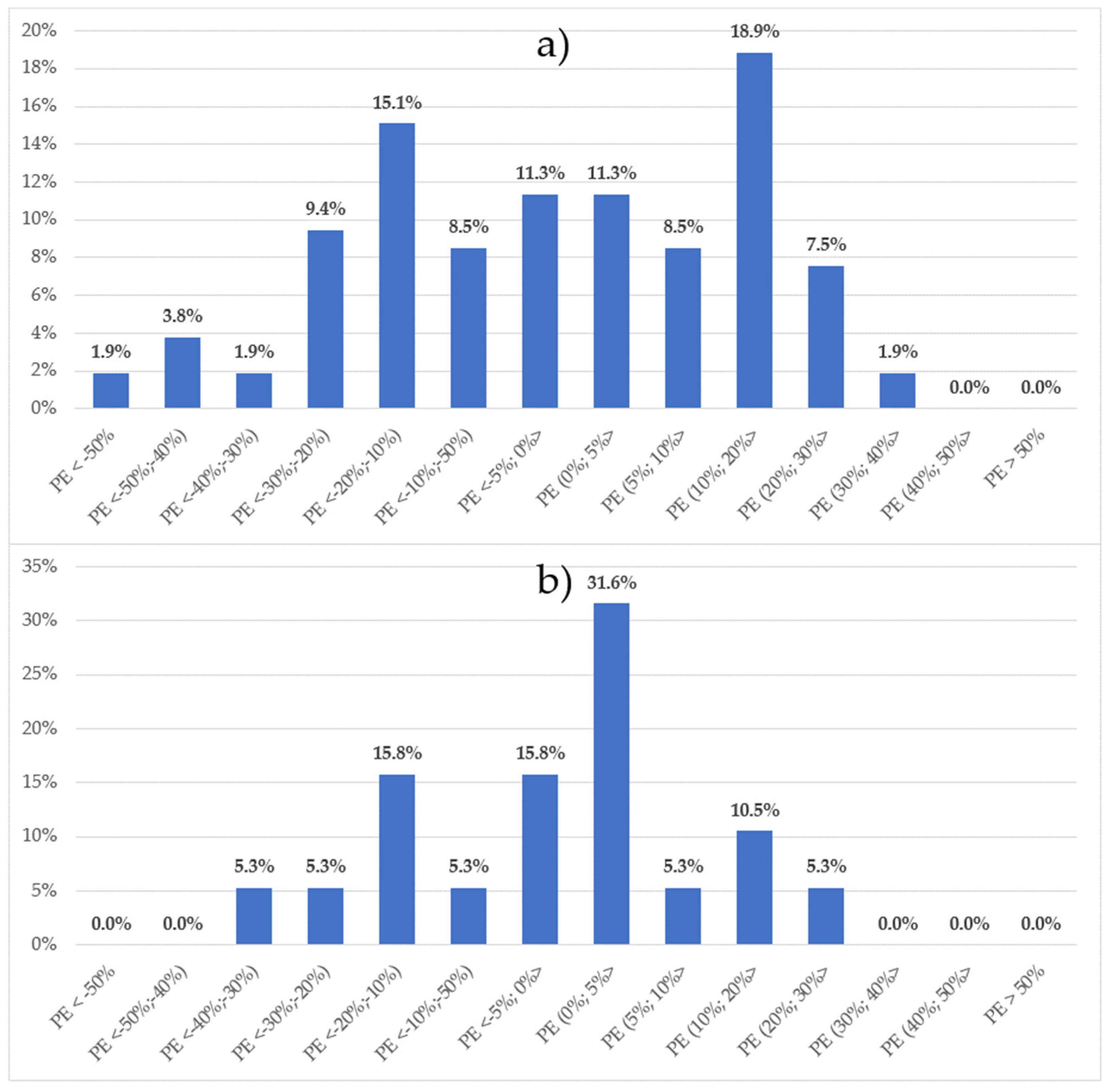
Figure 5 and Figure 6 present distributions of percentage errors PE^p, computed using Equation (15) and categorized within the ranges shown on the horizontal axes for the SAV_ENS and GAV_ENS models, respectively;

An analysis of the PE^p distributions allows us to select the SAV_ENS model as the one that is slightly more stable when comparing training and testing errors. The shares of PE^p within the range <−30%; 30%> were as follows:

• For SAV_ENS: 90.6% for the L&V subset and 94.7% for the T subset;
• For GAV_ENS: 84.0% for the L&V subset and 94.7% for the T subset.

Table 9. Values of general predictive performance measures for the EoNN models.

EoNN	RMSEL&V	RMSET	MAPEL&V	MAPET	max {APEPL&V}	max {APEPT}
SAVENS	436.8	344.5	15.1%	9.3%	57.6%	29.6%
GAVENS	266.3	257.5	14.9%	9.9%	64.6%	31.3%

presents a summary and performance measures of the two developed models, specifically RMSE and MAPE values, as well as the maximum values of APE^p. The maximum values of APE^p, which are lower for the SAV_ENS model, confirm that its predictive performance is slightly better than that of the GAV_ENS model.

In general, it can be concluded that the obtained results are satisfactory. The developed predictive models provide cost estimates within the assumed and preferred range of accuracy for the majority of both training and, most importantly, testing cases. The model based on simple averaging performs slightly better and offers higher accuracy.

6. Discussion

As evident from the literature analysis, attempts to develop cost analysis models for sewerage projects have been made [19,20,21,22,23,24,25,26]. In comparison to the analyses presented in this article, it can be noted that the selection of cost predictors, in terms of their nature, is similar. However, it should not be forgotten that local construction market conditions and data availability also influence the research. The final set of cost predictors and their values strongly depend on the possibility of obtaining them, which results in some differences between the models presented in the literature.

Among the mentioned works, some are based on the use of ANN [25,26]. Unfortunately, it is challenging to compare the results of these studies with the findings of this research. The cited works used less data for training and testing, and the models are based on single networks. Most importantly, there is a lack of precise information about the types of neural networks used and essential details regarding the training and testing processes of ANN and the analysis of their performance.

Thus, it was decided, for the purpose of further assessing research results, to develop a benchmark model based on multiple regression using the classical least square method. The benchmark model is hereinafter referred to as MR. The general formula for predictions based on the MR model is provided below.

$$\widehat{y}={\beta }_0+{\sum }_j{\beta }_j{x}_j$$

(16)

where:

β₀, β_j—regression coefficients.

To ensure the comparability of the MR benchmark model with the models based on the EoNN approach developed during the research, the computation of coefficients β₀ and β_j was performed with the use of subset C, equivalent to the training subset for ANNs that became members of SAV_ENS and GAV_ENS (including cases used for learning and validation processes). For testing the MR model, subset T was used. Below are the coefficients obtained from the regression analysis, along with the standard errors of estimation provided in the brackets.

β₀ = −5588.5 (1420.85); β₁ = 1064.6 (376.12); β₂ = −39,347.1 (62,376.80);

β₃ = 1414.0 (1025.67); β₄ = 2416.5 (727.67); β₅ = 2821.5 (548.23);

β₆ = 30.8 (235.41); β₇ = 240.0 (358.94); β₈ = 3329.0 (763.03); β₉ = 1340.1 (635.74);

β₁₀ = 38,154.7 (53,700.36); β₁₁ = 18,397.4 (20,636.69); β₁₂ = 36.9 (449.73)

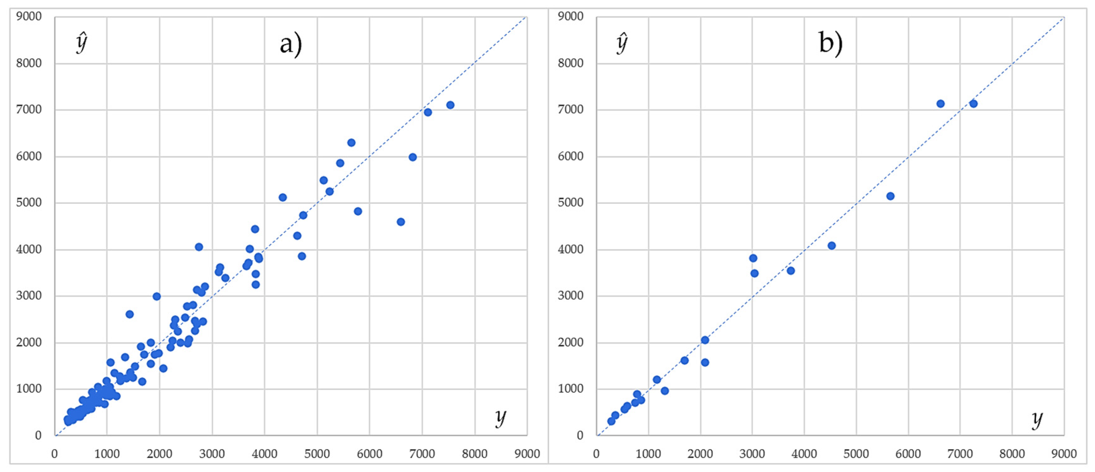
Figure 7 displays the results for the MR model in the form of a scatter plot of y and ŷ values (compare with Figure 3 and Figure 4).

Correlation coefficients R were computed in a similar manner as in the case of the SAV_ENS and GAV_ENS models;

• For MR: R = 0.926 for the C subset and R = 0.940 for the T subset;

When compared to the correlations computed for the developed EoNN-based models, the differences that occur are relatively insignificant. However, an analysis of the scatter plots and a comparison with those presented for EoNN-based models reveal greater dispersion and deviations from the line of perfect fit in the case of the MR benchmark model;

An analysis of the PE^p distributions for the MR benchmark model reveals the superiority of EoNN-based models. For MR, the shares of PE^p within the range <−30%; 30%> were as follows:

• 68.9% for the C subset and 73.7% for the T subset;

Table 10. Values of general predictive performance measures for the MR model.

	RMSEC	RMSET	MAPEC	MAPET	max {APEPC}	max {APEPT}
MR	647.04	743.31	29.5%	19.3%	81.9%	111.5%

provides a summary and performance measures for the MR benchmark model (compare with Table 9).

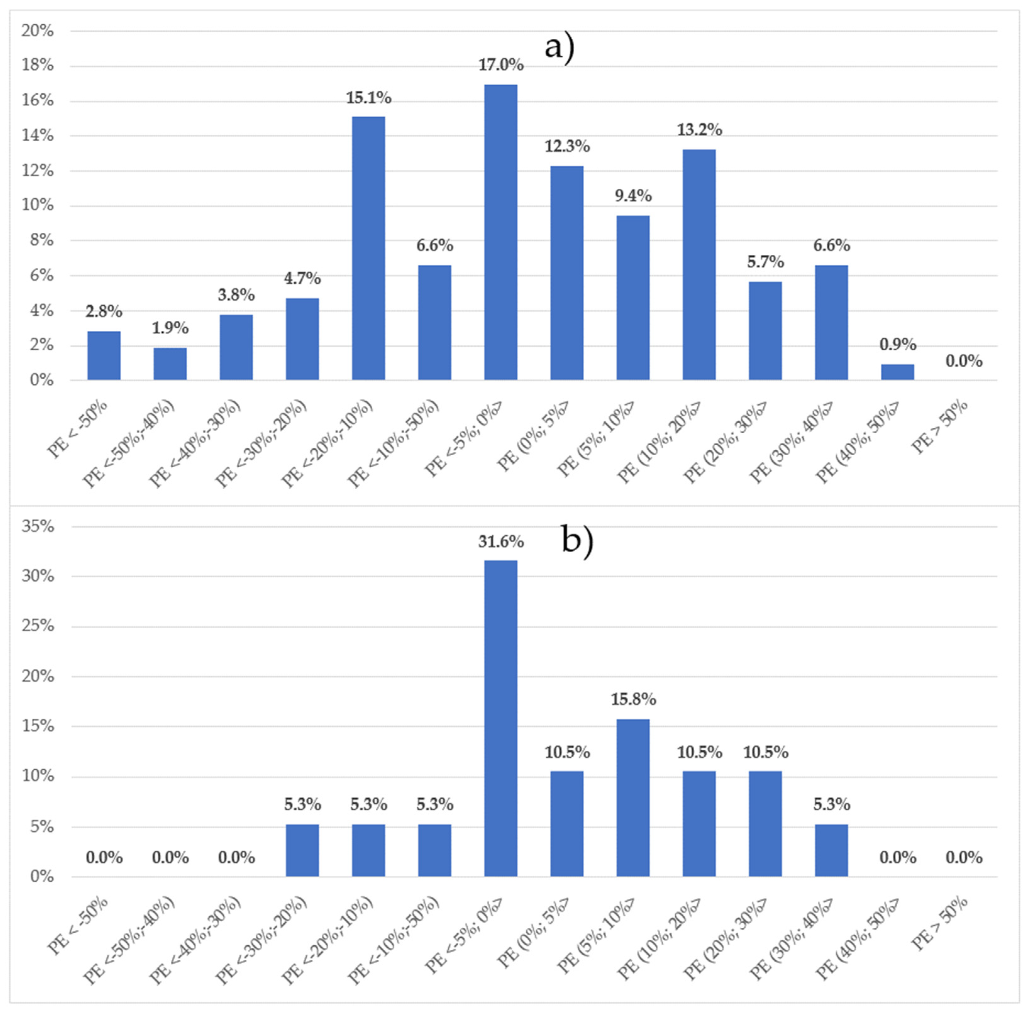
Figure 8 depicts the distributions of percentage errors PE^p, similar to those presented for the SAV_ENS and GAVE_NS models (compare Figure 5 and Figure 6).

A comparison of the values in Table 9 and Table 10 reveals that the overall prediction performance of the MR model based on linear regression is weaker than the performance of EoNN-based models (specifically, the SAV_ENS and the GAV_ENS models) developed by this study for the purposes of sewerage projects construction costs prediction.

As described in the preceding section, the research results are satisfactory. The models developed using EoNN have demonstrated their ability to predict construction costs for sewerage projects, for either stormwater runoffs or wastewater runoffs, with acceptable accuracy, meeting the requirements of the expected range of errors in over 90% of the test cases. The SAV_ENS and GAV_ENS models exhibit improved predictive capabilities when compared to individual ANNs, selected to be the ensemble members, used as standalone models. This improvement can be attributed to the effective compensation of errors inherent in single ANNs when they are combined within the ensemble. Moreover, combining several ANNs provides more objective cost predictions, as a certain bias of single ANNs acting in isolation is inevitable due to the size of the training set used in the course of research.

The two applied approaches, specifically simple averaging for the SAV_ENS model and generalized averaging for the GAV_ENS model, differ in terms of the computational effort required to determine the weights of the member ANNs. The first approach is straightforward—in fact, it involves taking the arithmetical average of predictions as the EoNN output. In contrast, the second approach demands more effort. However, this can be efficiently accomplished using a calculation sheet or through programming and automation of computations. The generalized averaging approach, with its weight optimization, allows for a more nuanced differentiation of the influence of individual member ANNs on the final cost prediction. In summary, both approaches are user-friendly and easily applicable.

The key advantage of an ensemble-based approach, as affirmed by the research presented, lies in the efficient utilization of training and testing efforts across ANNs rather than focusing solely on a single network. This observation carries particular significance in the contemporary context, where rapid progress in computer technology and the availability of efficient software enables the exploration of numerous networks within a relatively short timeframe.

It is also essential to acknowledge the limitations of the developed models. Firstly, the models are explicitly tailored to the specific local conditions. This is a consequence of the evident fact that the data used for training and testing were collected in the Czech Republic. However, it is worth noting that the application of the proposed approach in other locations is feasible, making the conceptual framework broadly applicable. The second significant limitation stems from the data update scheduled for mid-2023. In this regard, the proposed model and approach do not provide dynamic and automatic adjustment to cost variations over time. This issue will be the subject of further research.

In summary, the novelty of the proposed model lies in its use of AI tools, specifically ANNs, and the combination of trained ANNs in the form of an ensemble to achieve objective cost predictions for sewerage construction projects. The literature review indicates that this approach is original, with no prior research reporting the development of similar models for such projects.

7. Summary

The research resulted in the development of two original predictive models capable of forecasting the construction costs of sewerage projects based on ensembles of neural networks. Based on the applied artificial intelligence tool’s training capacity, influenced by the collected data, features, and characteristics of the analyzed projects, as well as the underlying assumptions, the developed models demonstrate the capability to forecast construction costs for either wastewater or stormwater runoffs, excluding combined runoffs.

The ensembles mentioned above consist of five different MLP-type ANNs. The outputs of these ANNs are combined using two alternative approaches: simple averaging and generalized averaging. Although the predictive performances of the two EoNN-based models are comparable, the one based on simple averaging appears to offer slightly better results. The accuracy of cost predictions is satisfactory. Especially for the model based on simple averaging, that is, the SAV_ENS model, more than 90% of cost prediction cases, both for training and testing, meet the accuracy requirements with percentage errors falling within the acceptable range of <−30%; 30%>. While the developed model has its limitations, it holds potential applications in estimating the costs of construction for sewerage projects in the Czech Republic. Furthermore, the proposed general approach may find applicability in other countries, although the models should be adapted and trained using locally collected data.

Future studies will involve further data collection and the development of models based on AI tools. Additionally, future research will focus on incorporating cost variability over time into these models in order to overcome existing limitations.