Identification of Dynamic Vibration Parameters of Partial Interaction Composite Beam Bridges Using Moving Vehicle

Abstract

The vibration response of a partial composite beam bridge under the influence of moving vehicular loads was investigated. Due to the coupling effect between the vehicle and the bridge, the vibration information of the vehicle encompassed the vibration information of the bridge. Consequently, the dynamic response of the vehicle could be utilized to extract the dynamic information of the composite beam. A moving mass-spring-damping system and composite beam elements considering interfacial slips were used for the interaction vibration of a vehicle-composite bridge. A finite element program for the interaction vibration analysis of the vehicle-composite beam bridge was developed. The program was used to extract the vibration information of the composite beam bridge by analyzing the vehicle displacement, velocity, and acceleration in the interaction vibration of the beam and the vehicle. Taking the Hangzhou Jiubao Bridge as the engineering background, the influences of structural parameters such as shear stiffness of connections, prestress magnitude, as well as vehicle parameters, including vehicle stiffness, damping, and mass, on frequency identification were analyzed. Furthermore, the influences of road roughness, disturbance force generated by vehicle random vibrations, and interference signals generated by signal transmission on frequency identification of the bridge were investigated.

1. Introduction

The natural frequencies of bridges play a crucial role in health monitoring. Continuous monitoring and analysis of these frequencies provide valuable insights for maintenance, repair, and ensuring the safety of bridges [1,2]. Damping ratio [3] and mode shape [4] are also used as indicators of structural health and damage. Conversely, the damage degree of a bridge structure can be evaluated by the dynamic characteristics of the bridge. The conventional approach for measuring the dynamic response of a bridge involves installing dynamic sensors on the bridge structure [5,6]. The damage of a bridge will lead to the change of its dynamic characteristics [7]. Vibration-based nondestructive testing has also been studied for many years [7,8,9,10]. Researchers have increasingly focused on measuring devices, analysis methods, and system identification techniques for bridge vibration modal characteristics [2,11,12].

To enhance work efficiency and reduce cost, an indirect method was proposed [13]. The vibration information of bridge can be extracted by analyzing the vibration information of the vehicle [14], and the influences of parameters, such as initial acceleration ratio, frequency ratio, and velocity, on bridge frequency identification were discussed. The authors in [1,12] took the square of acceleration as the information carrier of structural dynamic characteristics. Yang et al. [15] proposed a band-pass filter singular spectrum analysis method to filter vehicle frequency. Malekjafarian and Obrien [16] utilized short-term frequency domain decomposition to estimate the mode shape of the bridge based on the dynamic response of the vehicle. They introduced external excitation to the bridge while subtracting the signal from the continuous trailer axle of the vehicle’s traction, thereby mitigating the influence of roughness. Regarding parameter analysis, McGetrick et al. [17] highlighted that improved accuracy in bridge frequency estimation can be achieved at lower speeds and on flat pavement conditions. Studies have shown that the initial vehicle–bridge acceleration amplitude ratio plays a crucial role in identifying the frequency of a bridge [15,17]. Specifically, a smaller ratio of vehicle-to-bridge acceleration amplitude is conducive to the successful identification of the bridge frequency.

To the best knowledge of authors, the applications of the indirect method for composite beam bridges have not been reported. Further investigation is needed to evaluate the applicability of the indirect method to composite beams. To study the dynamic interaction between the moving vehicle and the composite bridge, the vehicle system can be simulated by moving load, moving mass, moving spring-mass, and moving spring-mass-damping models [14,18,19]. There are also some complex vehicle models [1,20,21]. Composite beam bridge sections are usually composed of two or more materials (usually steel and concrete), which can make full use of the mechanical properties of different materials. However, the influences of the shear connection and interfacial slips between different subcomponents on the identification of bridge frequency have not been investigated [22,23,24]. This study focused on the application of the indirect method in composite beams. The vibration frequency of composite beams was obtained through the utilization of the indirect method. In order to determine the optimal configuration of vehicle parameters, an analysis was conducted to assess the influence of various parameters, including vehicle mass, vehicle stiffness, vehicle damping, vehicle speed, shear connection stiffness, and prestress of the tendon. Furthermore, the influences of environmental disturbances were also discussed.

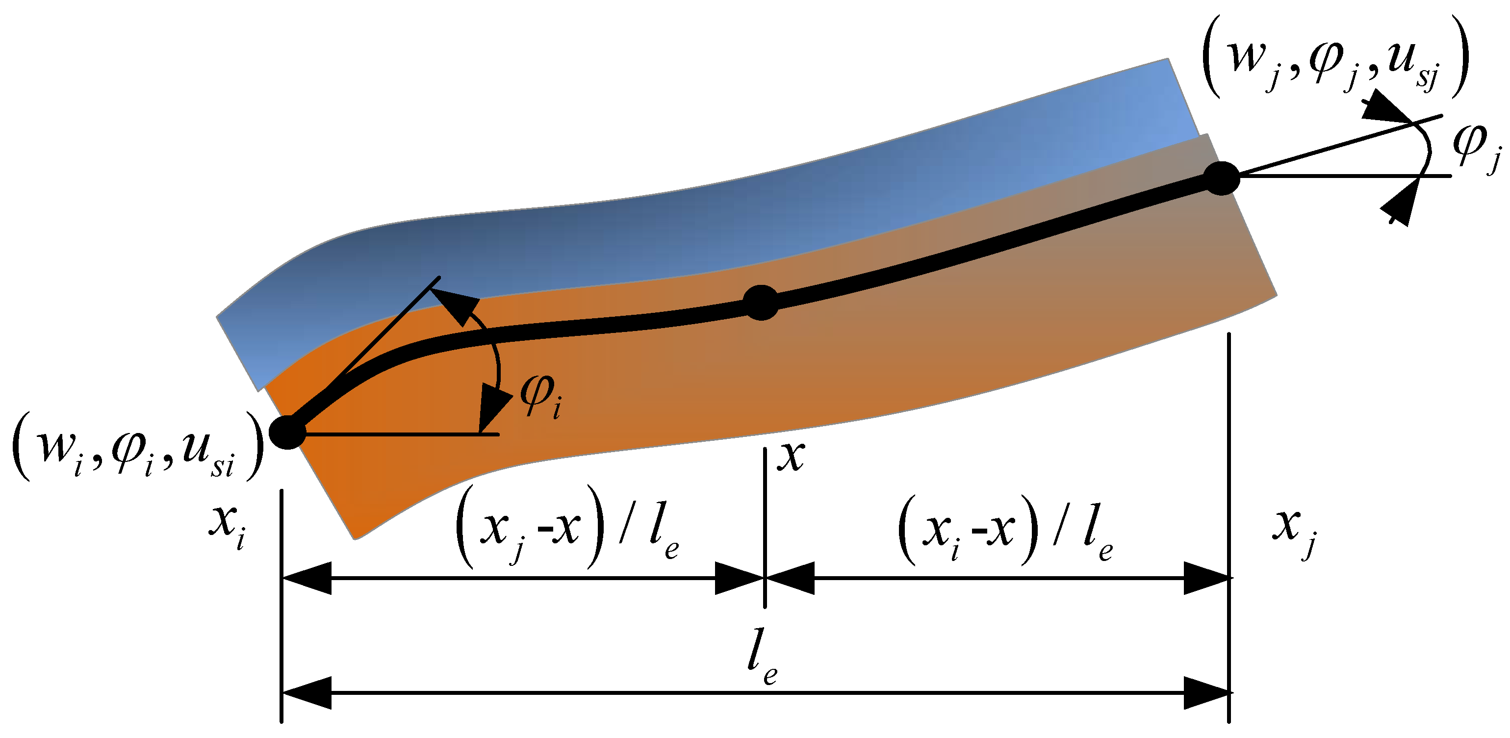
2. Vehicle-Composite Beam Bridge Interaction Vibration

Here is a basic introduction to the establishment and solution of the interaction vibration equation between the vehicle and the composite beam bridge. Bridges were simulated using planar beam elements due to their simplicity and efficiency. As shown in Figure 1, a composite beam element, which accounted for interfacial slip, was utilized in the dynamic analysis to ensure simplicity and efficiency [25,26]. The node displacements of composite beam elements are the deflection $w_i$, the rotary angle ${\phi }_i$, and the inter-interface slip $u_{si}$. The corresponding nodal forces are the axial force $F_{Ni}$, shear force $Q_i$, and bending moment $M_i$.

Due to the coupling effect of the axle, the vehicle induces forced vibrations, which are subsequently influenced by the vibrations of the composite beam bridge. Considering the overall vibration of both the vehicle and the bridge, the beam element incorporates an additional degree of freedom for the vehicle, in addition to the original six degrees of freedom.

The vehicle was simulated with a moving mass-spring-damper system, as shown in Figure 2. According to Hamiltonian’s principle, the energy equations can be written as:

$$\delta {\displaystyle {\int }_{{}_{t_1}}^{t_2}(L-R)dt=}\delta {\displaystyle {\int }_{{}_{t_1}}^{t_2}(T-U+W-R)dt=0}$$

(1)

where δ is the variation symbol, $L=T-U+W$, $T,U,W,R$ are the system kinetic energy, the system potential energy, the virtual work performed by the external forces, and the Rayleigh’s dissipation energy, respectively.

The revised Lagrange equations can be written as:

$$\frac{d}{dt}(\frac{\partial L}{\partial {\dot{u}}^e})-\frac{\partial L}{\partial u^e}-\frac{\partial R}{\partial {\dot{u}}^e}=0$$

(2)

which leads to the final system of equations as:

$$\left[\begin{array}{cc}{\mathbf{M}}^e& {\mathbf{M}}_c\\ {\mathbf{M}}_c^T& M_M\end{array}\right]\left\{\begin{array}{c}{\ddot{\mathbf{u}}}^e\\ \ddot{y}\end{array}\right\}+\left[\begin{array}{cc}{\mathbf{C}}^e+{\mathbf{C}}_M^e& {\mathbf{C}}_c\\ {\mathbf{C}}_c^T& C_M\end{array}\right]\left\{\begin{array}{c}{\dot{\mathbf{u}}}^e\\ \dot{y}\end{array}\right\}+\left[\begin{array}{cc}{\mathbf{K}}^e+{\mathbf{K}}_M^e& {\mathbf{K}}_c\\ {\mathbf{K}}_c^T& K_M\end{array}\right]\left\{\begin{array}{c}{\mathbf{u}}^e\\ y\end{array}\right\}=\left\{\begin{array}{c}{\mathbf{Q}}^e\\ Q_M\end{array}\right\}$$

(3)

in which, ${\mathbf{M}}_c$ = 0, $M_M$= $m_M$, ${\mathbf{C}}_M^e=\frac{c_M}{k_M}{\mathbf{K}}_M^e$, ${\mathbf{C}}_c=\frac{c_M}{k_M}{\mathbf{K}}_c$, $C_M$= $c_M$, ${\mathbf{K}}_M^e=\frac{k_M}{m_M}{\mathbf{M}}_M^e$. The explicit expressions of the matrices in the vehicle-composite beam bridge interaction vibration equation are described in detail in the reference [26].

After the elements stiffness matrix, mass matrix, and damping matrix are assembled into the global matrix, the dynamic response of the system can be solved by step-by-step integration. The key lies in establishing the recurrence relationship of the state vector from time t to time $t+\theta \Delta t$, where the displacement, velocity, and acceleration of the system, $U_{t+\Delta t}$, ${\dot{U}}_{t+\Delta t}$, ${\ddot{U}}_{t+\Delta t}$, satisfy the dynamic equation:

$${\rm M}{\ddot{U}}_{t+\Delta t}+C{\dot{U}}_{t+\Delta t}+K{U}_{t+\Delta t}=f_{t+\Delta t}$$

(4)

The solution method employed in this study is the Wilson-θ method, which assumes a linear variation within the interval $[t,t+\theta \Delta t]$, as follows:

$${\ddot{U}}_{t+\Delta t}={\ddot{U}}_t+\frac{\tau }{\theta \Delta t}({\ddot{U}}_{t+\theta \Delta t}-{\ddot{U}}_t)\hspace{1em}\hspace{1em}\hspace{1em}\hspace{1em}(0\le \tau \le \theta \Delta t)$$

(5)

The recurrence relations for acceleration, velocity, and displacement at time t and time $t+\theta \Delta t$ can be derived as follows:

$${\ddot{U}}_{t+\Delta t}={\alpha }_4(U_{t+\Delta t}-U_t)+{\alpha }_5{\dot{U}}_t+{\ddot{U}}_t$$

(6)

$${\dot{U}}_{t+\Delta t}={\dot{U}}_t+{\alpha }_7({\ddot{U}}_{t+\Delta t}+{\ddot{U}}_t)$$

(7)

$$U_{t+\Delta t}=U_t+\Delta t{\dot{U}}_t+{\alpha }_8({\ddot{U}}_{t+\Delta t}+2{\ddot{U}}_t)$$

(8)

${\ddot{U}}_{t+\Delta t}$ and ${\dot{U}}_{t+\Delta t}$ can be expressed in terms of $U_{t+\Delta t}$. Thus, the dynamic equation can be written as:

$$\tilde{K}{U}_{t+\theta \Delta t}={\tilde{f}}_{t+\theta \Delta t}$$

(9)

where

$$\tilde{K}=K+{\alpha }_{0}M+{\alpha }_{1}C$$

(10)

$${\tilde{f}}_{t+\theta \Delta t}=f_{t+\theta \Delta t}+M({\alpha }_0{U}_t+{\alpha }_2{\dot{U}}_t+2{\ddot{U}}_t)+C({\alpha }_1{U}_t+2{\dot{U}}_t+{\alpha }_3{\ddot{U}}_t)$$

(11)

in which, $\theta$, $\tau$, ${\alpha }_0$$~$${\alpha }_8$ are integral constants with specific values as follows: $\theta =1.4$, $\tau =\theta \Delta t$, ${\alpha }_0=\frac{6}{{\tau }^2}$, ${\alpha }_1=\frac{3}{\tau }$, ${\alpha }_2=2{\alpha }_1$, ${\alpha }_3=\frac{\tau }{2}$, ${\alpha }_4=\frac{{\alpha }_0}{\theta }$, ${\alpha }_5=-\frac{{\alpha }_2}{\theta }$, ${\alpha }_6=1-\frac{3}{\theta }$, ${\alpha }_7=\frac{\Delta t}{2}$, ${\alpha }_8=\frac{\Delta t^2}{6}$.

Based on Equations (5)–(11), given the initial state vectors $U_{t+\Delta t}$, ${\dot{U}}_{t+\Delta t}$, ${\ddot{U}}_{t+\Delta t}$, the state vector of the axle system at each moment can be obtained through step-by-step integration.

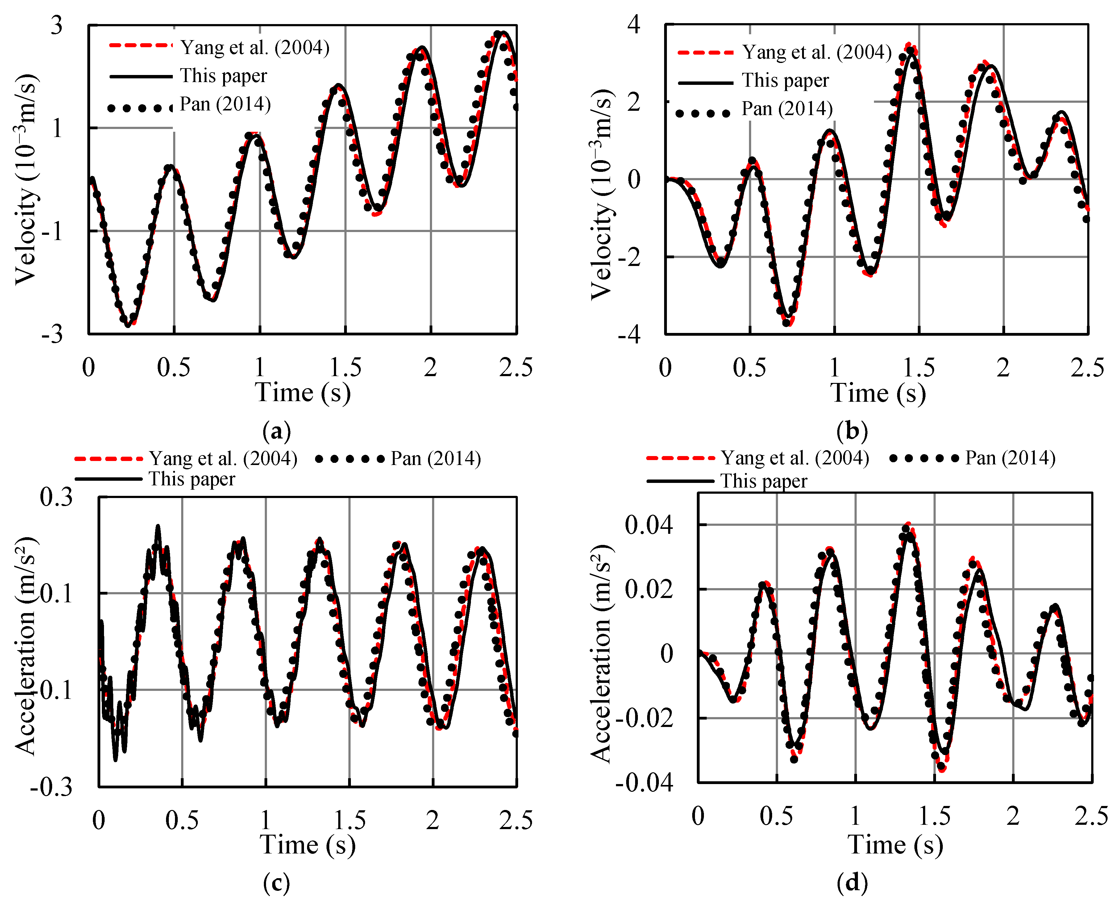
3. FE Method Validation

A finite element program was implemented using MATLAB, and a simulation model was employed and tested to verify the accuracy of the proposed method used in this paper. The parameters of the bridge structure were the same as that in Yang et al. [13]. The material and geometric characteristics are composite beam length L = 25 m, moment of inertia I = 0.12 m⁴, mass per unit length m = 4800 kg/m, and elastic modulus E = 27.5 GN/m². The two sub-beams were of the same shape and size, with a cross-sectional area of 2.0 m². The shear stiffness was set to a large value of 5 × 10⁷ MPa, indicating a nearly perfectly bonded structure. The vehicle mass m_v = 1200 kg, the spring stiffness k_v = 500 kN/m, and the damping was assumed to be zero. The vertical displacement, vertical velocity, and vertical acceleration of the vehicle, as well as the vertical velocity and vertical acceleration at the mid-span of the composite bridge, were selected for comparison, as shown in Figure 3. It can be found that the dynamic response results obtained using the method presented in this paper show good agreement with those reported in the existing literature [13,27].

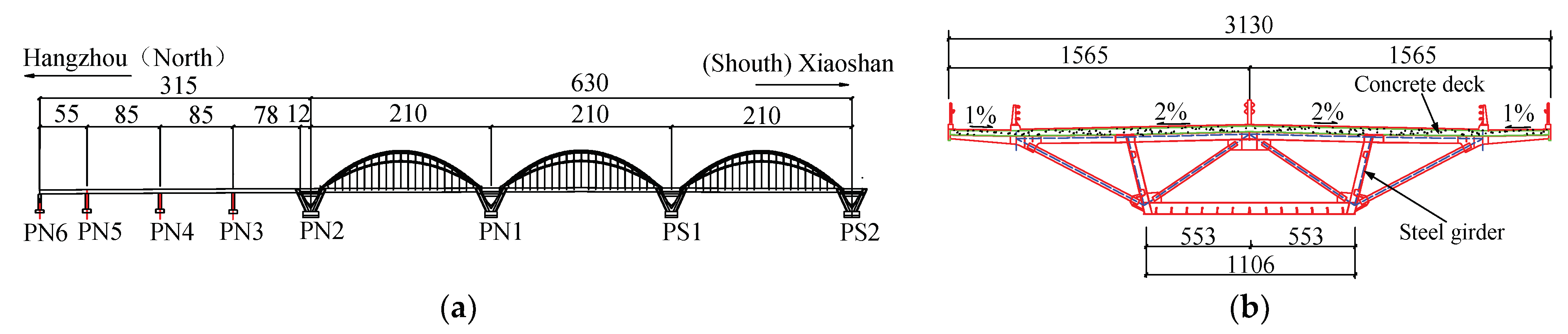
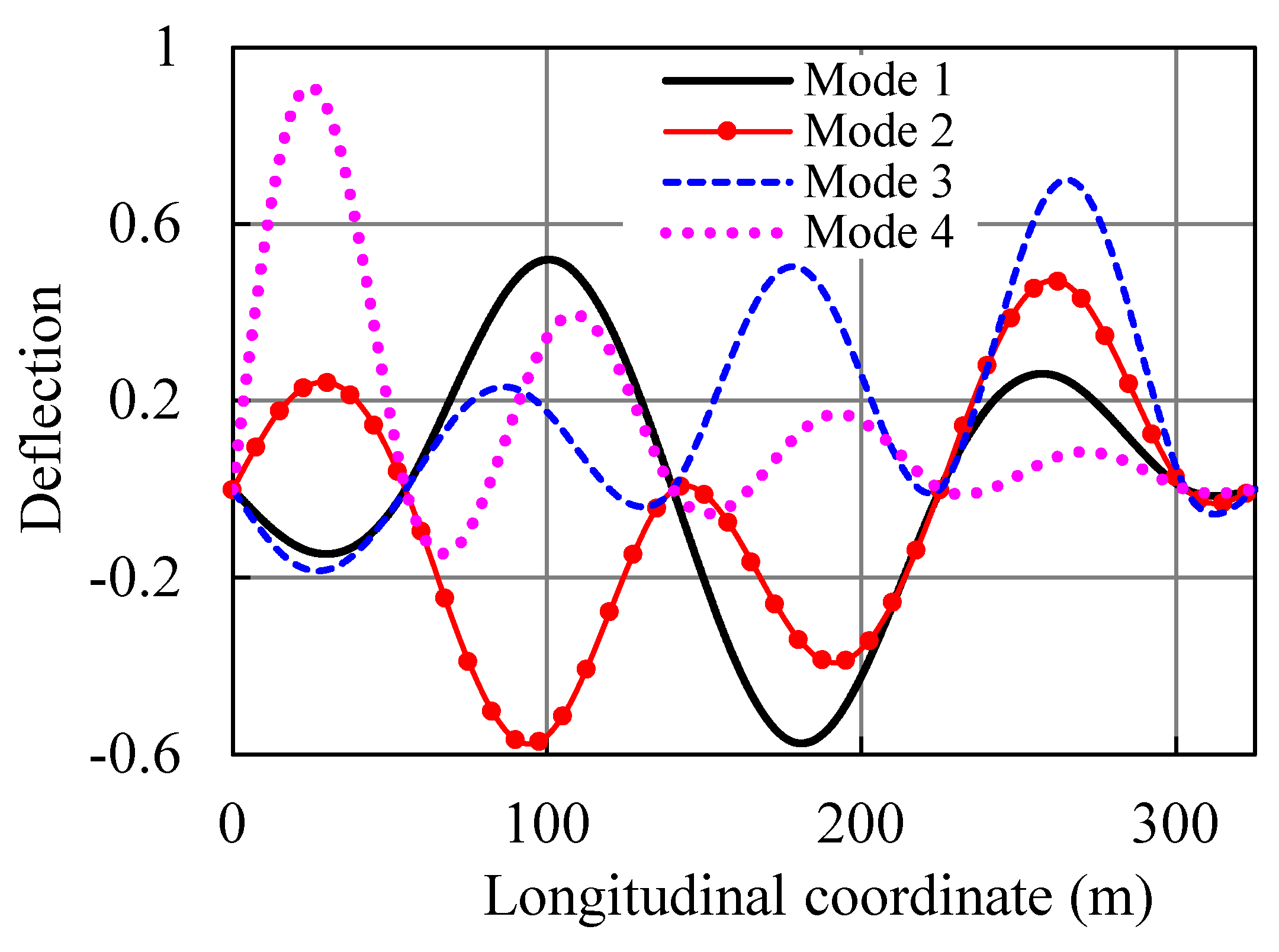
4. Numerical Application to Jiubao Bridge

Jiubao Bridge is one of the ten largest bridges over the Qiantang River. Its total length is 1855 m. The main bridge is a continuous composite beam-steel arch bridge, and the approach bridge has a constant section with spans of 85 m. The whole span arrangement is as follows: 55 m + 2 × 85 m + 78 m + 21.785 m (northern approach) + 3 × 210 m (main bridge). The span layout of Jiubao Bridge is shown in Figure 4a. In this paper, the northern approach bridge was the focus.

The Jiubao northern approach bridge is a multi-span continuous composite bridge. Its composite girders consist of a concrete deck and steel U-shaped girders. A typical cross section of the Jiubao northern approach bridge is shown in Figure 4b. The characteristic cylinder strength of concrete was 32.4 MPa, and the modulus of the concrete was 34.5 GPa. The shear stiffness of the studs was calculated and was equal to 5138.2 MPa. The influence of axial forces of the six post-tensioned tendons on the dynamic response was also included in the numerical analysis. The axial force value of each prestressed tendon applied on the composite beam was 3795.2 kN. The mass of the test vehicle was m_v = 35,000 kg, the stiffness k_v = 11,667 kN/m, the damping ratio ξ_v = 0.2, and the vehicle speed was 10 m/s.

The vertical displacement and the acceleration at the middle of the second span were subjected to Fourier transform to obtain the spectrogram. As shown in Figure 5, the vibration frequency could be obtained. Figure 6 shows the vertical displacement and acceleration of the vehicle, along with their corresponding spectrograms. Under the influence of the vehicle’s driving frequency, multiple bifurcation peaks appeared in the spectrogram. The average value of the bifurcation peaks corresponded to the vibration frequency of the bridge. The comparison results of the frequency spectrum analysis of the vehicle and bridge signals, along with the structural vibration frequency obtained from the natural vibration analysis of the bridge itself, are shown in

Table 1. The first 4 natural frequencies of the northern approach of Jiubao Bridge.

Order	Test Values	FE (Free Vibration)	FE (Force Vibration-Bridge)	FE (Force Vibration-Vehicle)	Relative Error-Free Vibration (%)	Relative Error-Vehicle (%)
1	1.39	1.40	1.38	1.40	1.06	0.72
2	1.83	1.98	1.97	1.97	7.93	7.61
3	2.39	2.61	2.58	2.58	9.12	8.14
4	3.39	3.51	3.51	3.52	3.55	3.77

. The first four mode shapes of the deflection for the northern approach bridges are shown in Figure 7. These mode shapes were obtained through free vibration analysis.

It can be seen from Table 1 that there was good agreement between the test values and the results of the finite element analysis for the first four-order frequencies. The relative error of the fundamental frequency obtained with the indirect method was only 0.72%, while the third-order frequency exhibited a relatively larger value within 10%. The relative errors were calculated with respect to the test values. Results showed that determining the vibration frequency of the composite beam bridge from the vehicle’s vibration is indeed feasible.

The influence of the duration of vehicle running time on the indirect identification results was also discussed. With the increasing running time of the vehicle, it is observed in Figure 8 that the peak spacing of the acceleration spectrum remained relatively unchanged, but the peaks gradually became larger and approached a fixed value, and bifurcation occurred at each peak point. Compared to short-term spectrograms, long-term spectrograms were easier to identify, and the frequency identification became clearer as the duration of vehicle running time increased.

5. Parameters Study

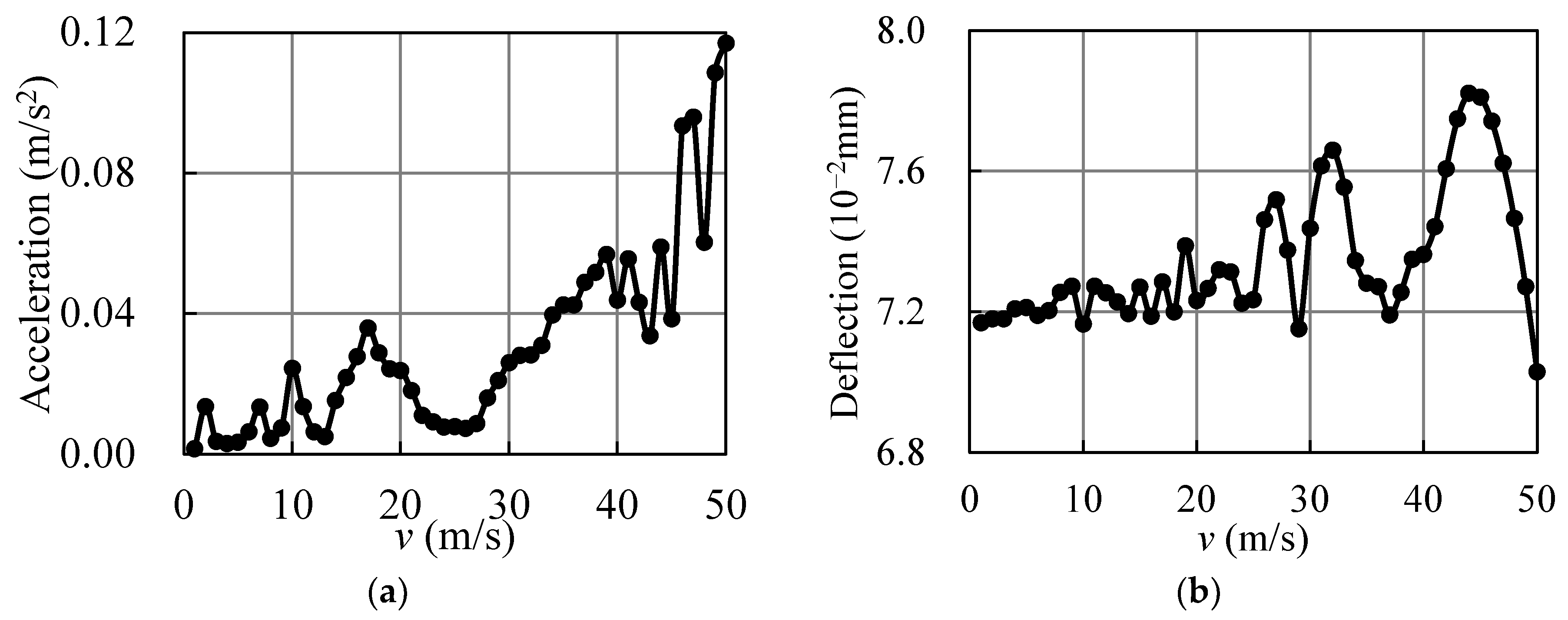
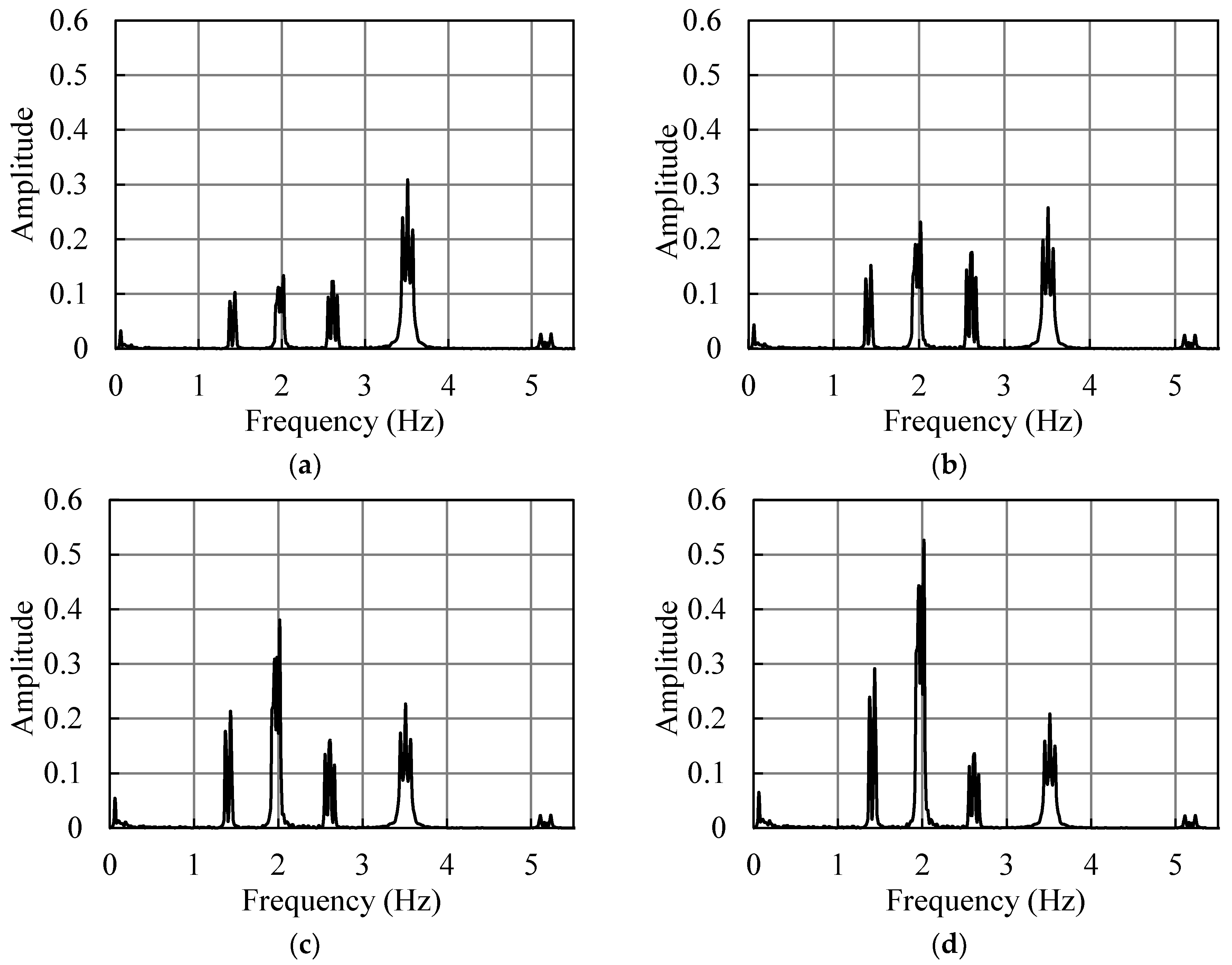
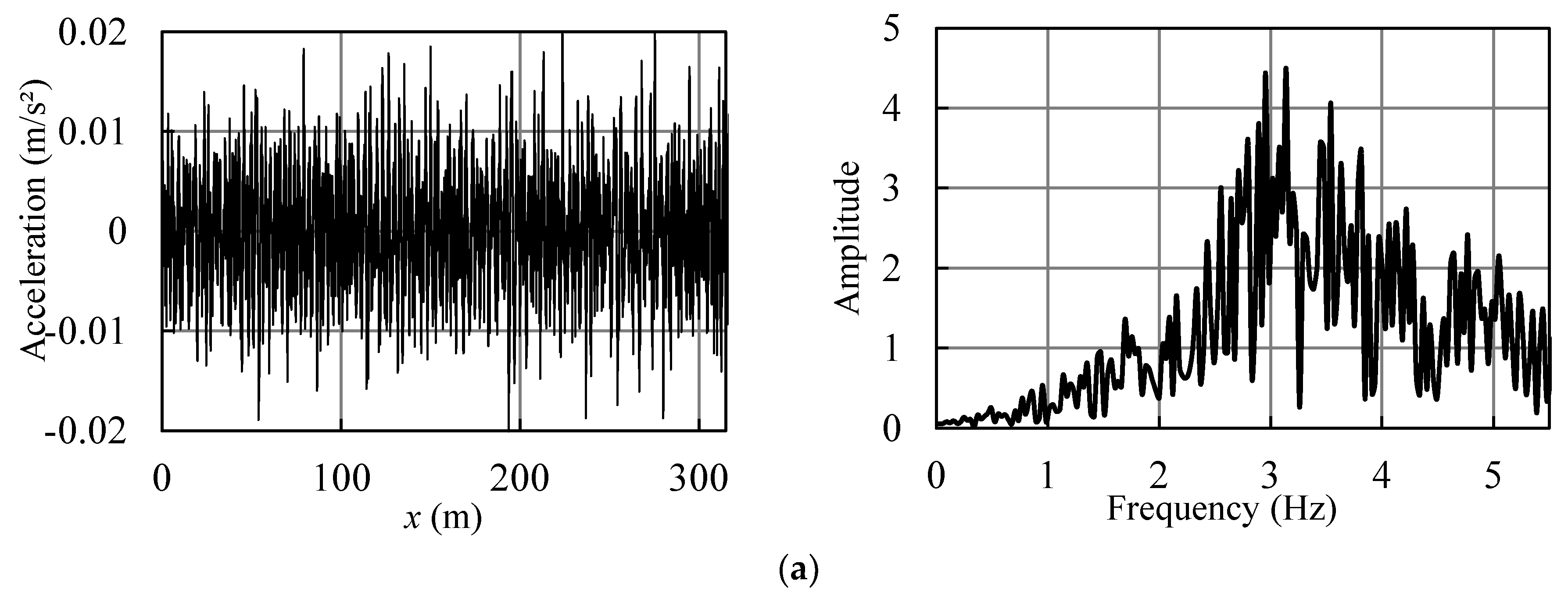
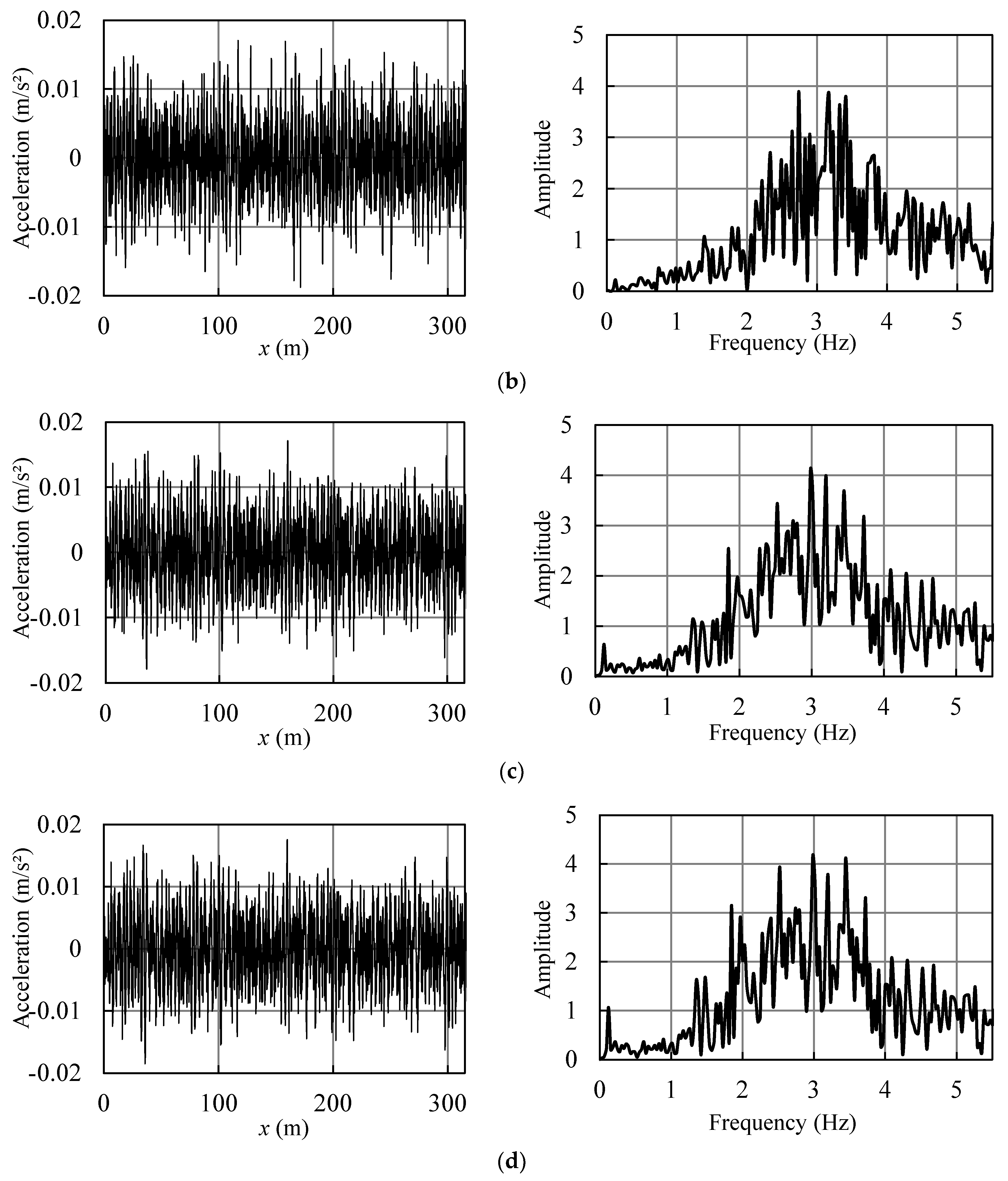
5.1. Influence of Moving Speed of Vehicle

The influence of moving speed on the vehicle acceleration and its corresponding acceleration spectrum are shown in Figure 9 and Figure 10, respectively. The results indicate that, at lower speed values, the frequency could be easily and clearly determined. As the vehicle speed increased, the influences of the driving frequency of the vehicle became more pronounced, and the peak spacing of the amplitude in the spectrogram became larger. Excessive vehicle speed led to the overlapping of peaks of adjacent order frequencies, making frequency identification challenging.

As the vehicle speed increased, the maximum acceleration of the vehicle also increased approximately linearly, as shown in Figure 11. The maximum amplitude of acceleration spectrum initially exhibited a linear increase within a small range and subsequently fluctuated between 0.2 and 0.4. Meanwhile, Figure 12 demonstrates that the maximum mid-span displacement of the composite beam did not consistently increase with the rise in vehicle speed. Instead, it exhibited a fluctuating upward trend.

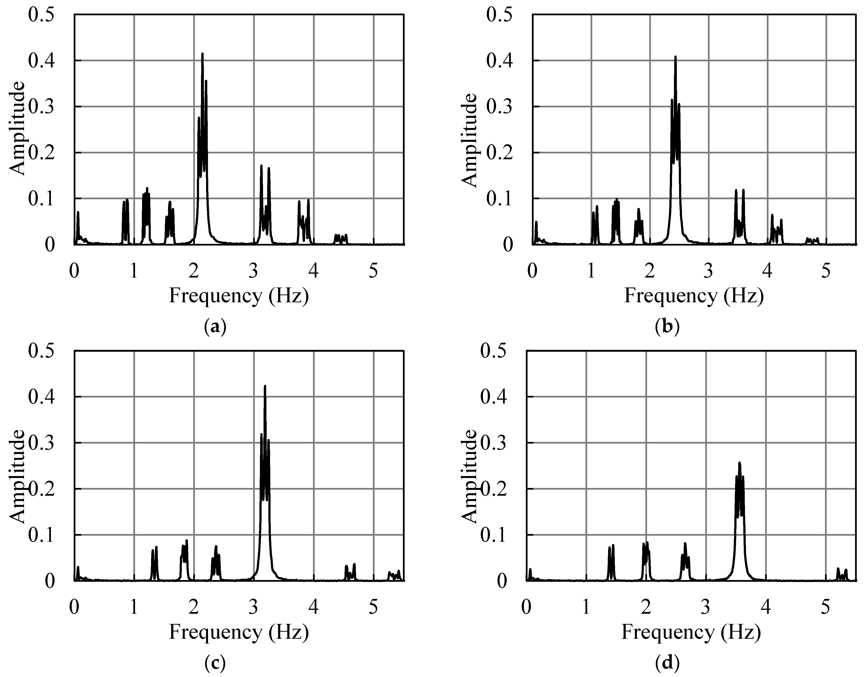
5.2. Influence of Vehicle Stiffness

Figure 13 illustrates the impact of vehicle stiffness on the acceleration spectrum. In the simulation model, the vehicle mass (m_v) was set to 1200 kg, the damping ratio (ξ_v) was 0.2, and the vehicle speed of 5 m/s was kept constant. As the vehicle stiffness (k_v) increased from 100 kN/m to 400 kN/m, the peak amplitude of the fundamental frequency of the composite beam bridge decreased, while the peak amplitude of the higher-order frequencies increased to varying degrees. Lower stiffness values facilitated the identification of fundamental frequencies, whereas higher stiffness values were more effective in capturing higher-order frequencies.

5.3. Influence of Vehicle Damping

The influence of the vehicle damping ratio on the acceleration spectrum is shown in Figure 14. The vehicle mass m_v = 1200 kg, the vehicle stiffness k_v = 500 kN/m, and the vehicle speed 5 m/s was kept constant. The results demonstrate that, as the damping ratio (ξ_v) increased from 0.02 to 8, the peak amplitude values of the first four-order natural frequencies in the acceleration spectrum all exhibited varying degrees of decrease. This decrease was particularly pronounced for the fourth-order frequency. If the amplitude of the high-order frequency is excessively large, it can make the identification of the fundamental frequency challenging. Therefore, for the purpose of fundamental frequency identification, a higher damping ratio can help reduce the amplitude of the high-order frequency, thereby making the fundamental frequency more prominent and easier to identify.

5.4. Influence of Vehicle Mass

The influence of vehicle mass was also investigated, as shown in Figure 15. With the increase in vehicle mass, the peak amplitudes of the first and second-order frequencies in the composite beam acceleration spectrum increased, while those of the third- and fourth-order frequencies decreased. For fundamental frequency identification, increasing the vehicle weight effectively amplified the spectrum amplitude of the fundamental frequency compared to higher-order frequencies.

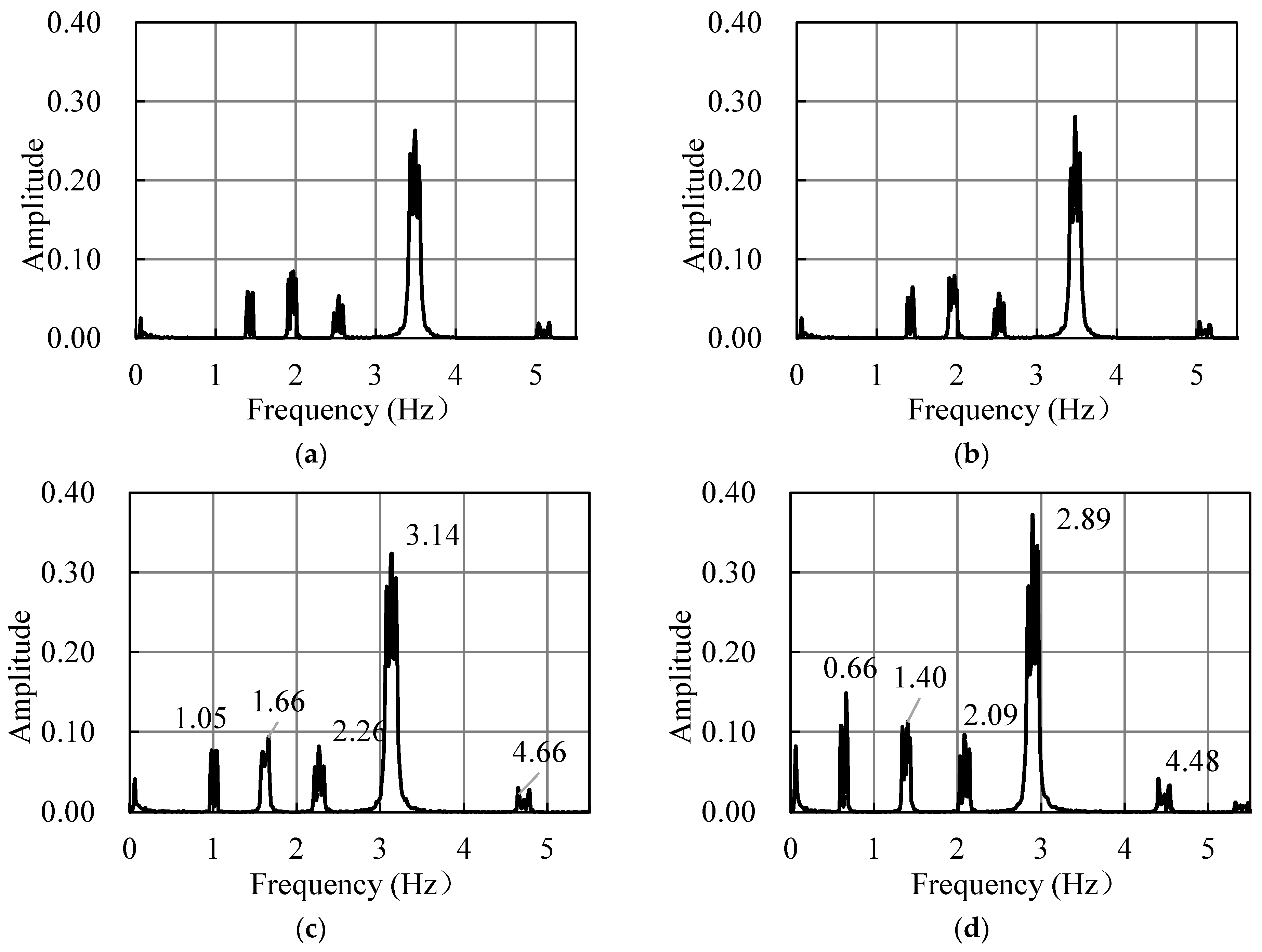
5.5. Influence of Shear Stiffness

The influence of shear stiffness on the acceleration spectrum was subsequently investigated. The information about the composite beam was the same as the previous Jiubao northern approach bridge. Only the shear stiffness of the composite beam was analyzed with k_s = 10 Mpa, k_s = 100 Mpa, k_s = 1000 Mpa, and k_s = 10,000 Mpa. The vehicle mass m_v was 1200 kg, the vehicle stiffness k_v was 500 kN/m, the vehicle damping ratio ξ_v was taken as 0.2, and the vehicle speed v was 5 m/s. The acceleration spectrums for the four shear stiffness values are shown in Figure 16. The results indicate that, as the shear rigidity increased, the peak point gradually shifted to the right. This suggests that the inherent frequency of the bridge gradually increased, which is consistent with the structural mechanical property. In the range of 10–1000 Mpa, the spectrum amplitude of the first four frequency peaks remained relatively constant, but at 10,000 Mpa, the spectrum amplitude of the fourth-order frequency slightly decreased. Higher-order frequencies (e.g., the fifth, sixth, and seventh frequencies shown in Figure 16a) significantly decreased in spectrum amplitude as the shear stiffness increased. This indicates that higher-order frequencies of the bridge are more easily excited when the shear stiffness is low.

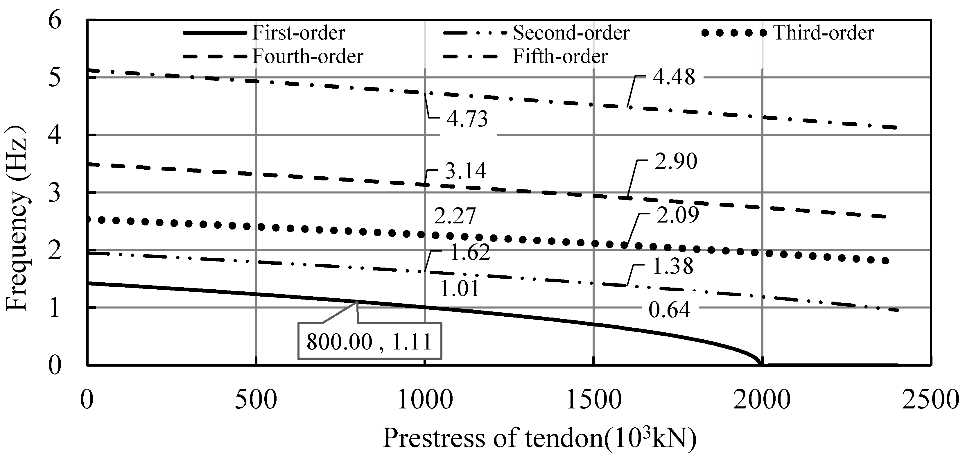
5.6. Influence of Prestress of Tendon

This section discusses the influence of prestress variations on the acceleration spectrum. Similar to the shear stiffness of connections, the prestress of the tendon is also a structural parameter of the composite beam itself. The composite beam was the same as the previous Jiubao northern approach bridge, with the only change in prestress magnitude F_P for the composite beam, taking F_P = 10² N, F_P = 10⁴ kN, F_P = 10⁶ kN, F_P = 1.6 × 10⁶ kN for analysis. The following vehicle parameters remained the same: vehicle mass m_v = 1200 kg, stiffness k_v = 500 kN/m, vehicle damping ratio ξ_v = 0.2, and vehicle velocity v = 5 m/s. The acceleration spectrum under the four prestress levels are shown in Figure 17. With the increase of prestress, the overall acceleration spectrum of the composite beam shifted to the left, indicating a decrease in frequency with increasing prestress. This observation is consistent with the results of the free vibration analysis, as illustrated in Figure 18. The amplitude of the spectrum slightly increased with the increase of prestress, but the change was not significant.

In practical applications, the identified bridge frequency from the indirect method can be compared with the prestress-frequency curve obtained from free vibration analysis to calculate the loss of prestress. For example, if the bridge is designed with a prestress of 10⁶ kN, and the identified change in the bridge’s fundamental frequency is 1.11 Hz, which corresponds to 0.8 × 10⁶ kN on the prestress-frequency curve, the predicted prestress loss would be about 20%. However, it is important to note that this example provides only one application scenario considering the variation in prestress. In actual practice, the frequency change of the bridge should take into account other factors that can cause stiffness variations, and the accuracy of the analysis should meet the required specifications.

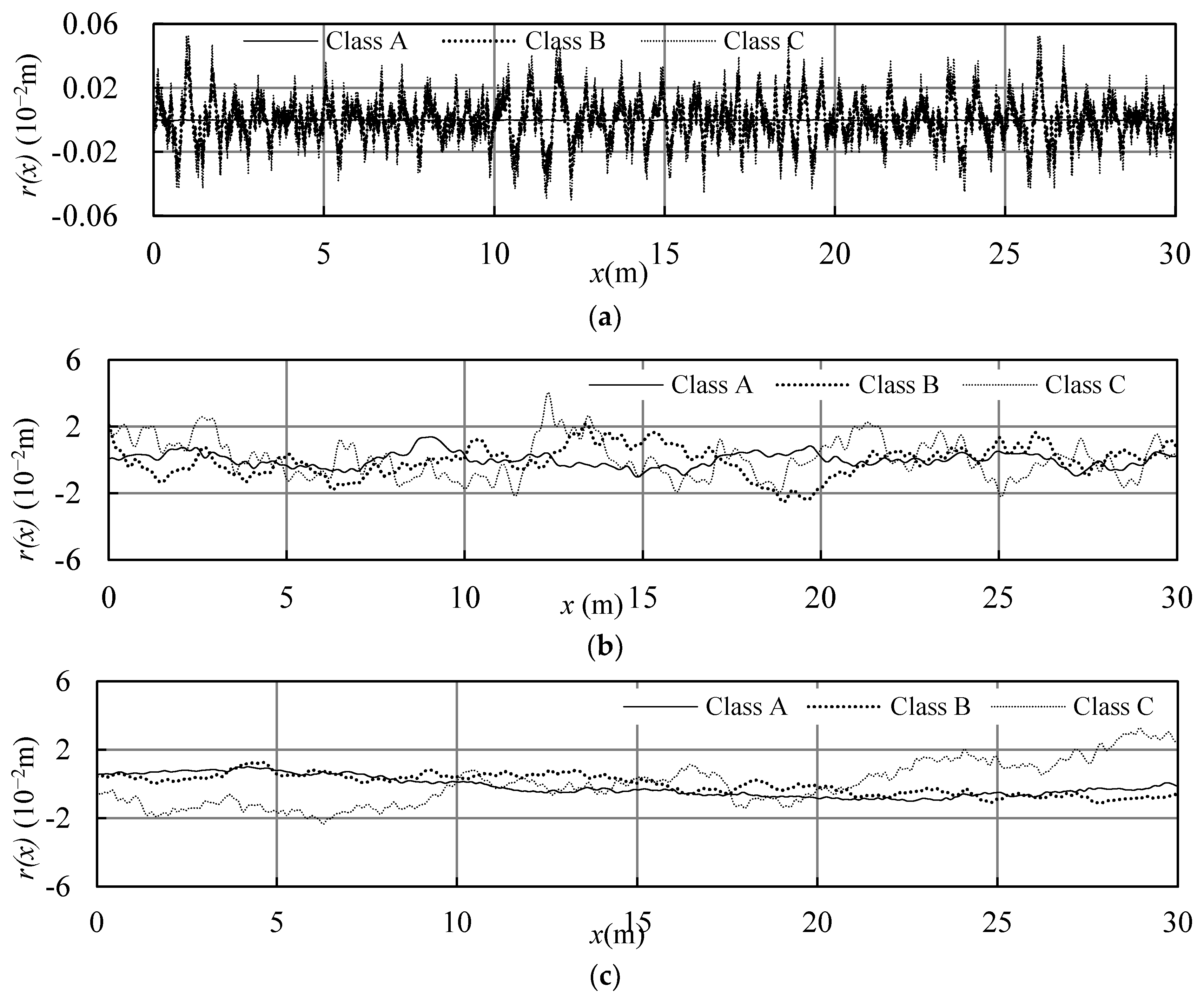
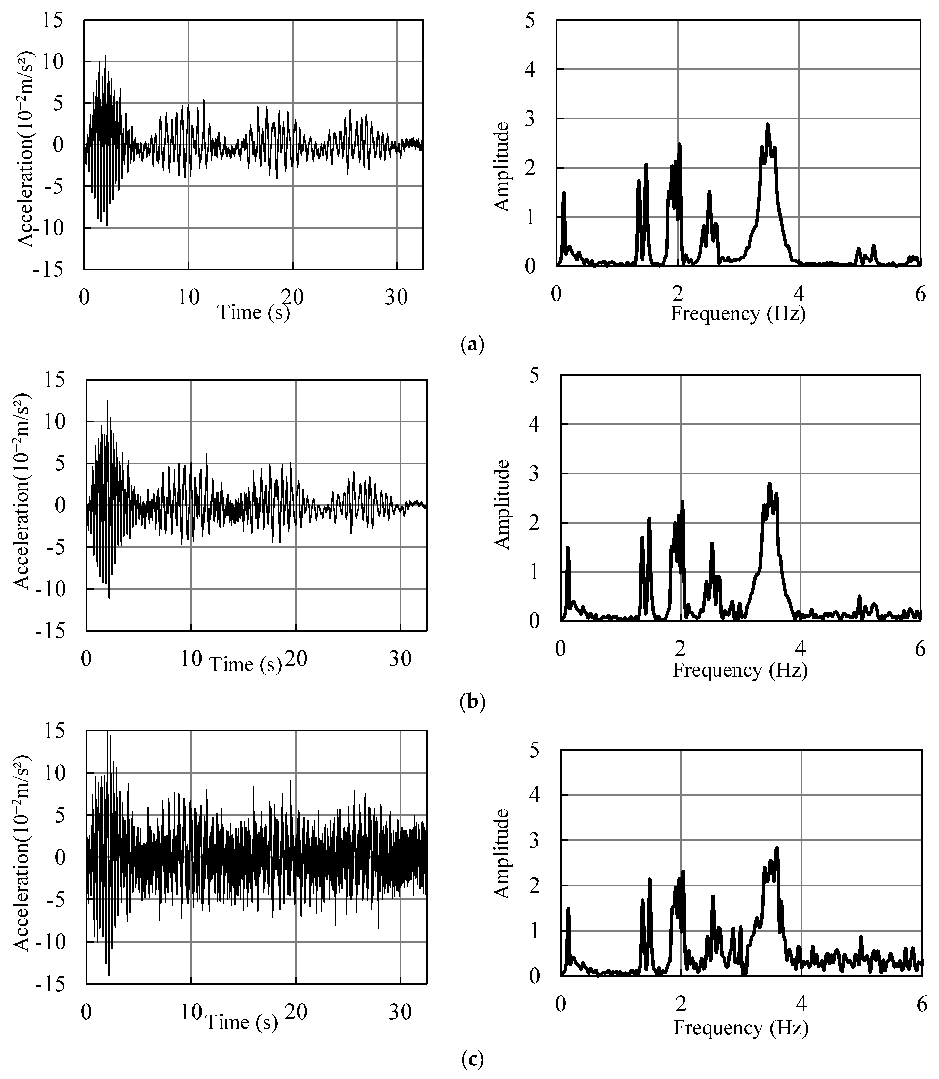
5.7. Influence of Pavement Roughness

5.7.1. Pavement Surface Roughness Generation Method

There are several methods available for simulating pavement unevenness, with the power spectral density (PSD) method being the most common. According to ISO-8608 [28], the general form of the PSD function $G_q\left(n\right)$ is as follows:

$$G_d\left(n\right)=G_d\left(n_0\right){\left(\frac{n}{n_0}\right)}^{-w}$$

(12)

where n denotes the spatial frequency per meter. $n_0$ is the reference spatial frequency, and $n_0$ = 0.1 cycles/m. w denotes the exponent of the fitted PSD function.

Given the power density of the pavement, harmonic superposition can be used to generate different grades of uneven pavement.

$$r\left(x\right)={\displaystyle {\sum }_i^{}{d}_i\cos \left(n_{S,i}+{\theta }_i\right)}$$

(13)

$$d=\sqrt{2G_d\left(n\right)\Delta n}$$

(14)

where $∆n$ is the sampling interval of the spatial frequency, d is the amplitude of each class of pavement, and θ is a randomly assigned phase angle.

In ISO-8608 [28], the recommended $G_q\left(n\right)$ values for grades A, B, and C of road surfaces were 16 × 10⁻⁶ m³, 64 × 10⁻⁶ m³, and 256 × 10⁻⁶, respectively. The amplitude of roughness recommended in ISO-8608 [28] was too large to be compatible with the road roughness from the field. In line with this, Yang et al. [29] proposed that the corresponding $G_q\left(n\right)$ values for the A, B, and C pavements were 0.001 × 10⁻⁶ m³, 8 × 10⁻⁶ m³, and 16 × 10⁻⁶ m³, respectively. Meanwhile, in Pan [27], the corresponding $G_q\left(n\right)$ values for the three different grade C pavements were 0.62 × 10⁻⁶ m³, 2.5 × 10⁻⁶ m³, and 10 × 10⁻⁶ m³, respectively.

To assess the influence of various parameters on simulating road surface unevenness, three representative pavement models were selected for comparison. The parameters of these models were sourced from Yang [29], Pan [27], and Chen [30], and they are referred to as Model 1, Model 2, and Model 3, respectively. Yang et al. [29] considered the vehicle frequency and the first three-order bridge frequency within the 0–40 Hz range. The range of the n value was 1–100 cycles/m. In contrast, Pan [27] focused on the bridge frequency within the 0–2 Hz range, selecting a spatial frequency range of 0.06–3 cycles/m. Chen [30] focused on the acceleration corresponding to road unevenness, without considering frequency identification. The road surface unevenness coefficient adopted values from ISO-8608 [28], and the selected spatial range was 0.01–5 cycles/m.

The influence of various parameters in the PSD function were further analyzed by considering a case study of a 30 m span bridge. The geometry and material parameters were the same as those provided in Yang et al. [29]. In the FE model, a high shear stiffness value of 5 × 10⁷ MPa was assigned, implying a state of near-perfect bonding within the structure. The material and geometrical properties were the length of the simply supported beam L = 30 m, cross-sectional area equals 2.0 m², the moment of inertia I = 0.175 m⁴, mass per unit length m = 1000 kg/m, and elastic modulus E = 27.5 GN/m². The mass of the vehicle m_v = 1000 kg, spring stiffness k_v = 170 kN/m, and a zero damping was assumed.

The road surface profiles generated using these three pavement roughness models are depicted in Figure 19. The road surface generated by Model 1 exhibited relatively dense spacing between the peaks, resulting in minor fluctuations across the entire bridge length. In contrast, the road surface profiles produced by the other two models showed relatively sparse peaks and larger fluctuations throughout the entire length. This difference can be attributed to the fact that Model 1 lacks small frequencies within the range of 0.01–1 Hz, which implies the absence of longer road surface waves.

In the case of a smooth road surface without unevenness, the various frequencies can be clearly identified, as shown in Figure 20. Among them, 0.07 Hz represents the vehicle driving frequency (v/L), 2.07 Hz represents the vehicle’s natural frequency, and the first three natural frequencies of the bridge are 3.87 Hz, 15.27 Hz, and 33.33 Hz, respectively. Due to the small driving frequency, the bifurcation effect at the peak of the acceleration spectrum was not prominent, and it can be approximated as a single main peak.

The time–domain acceleration curve and the acceleration spectrum considering the road surface with unevenness are shown in Figure 21. The Grade A pavement (with low unevenness) still allowed for the identification of bridge frequencies, with the fundamental frequency (3.87 Hz) being relatively prominent. Grade B and Grade C pavements only showed vehicle frequencies, while the bridge frequencies were masked by the frequencies caused by the pavement unevenness. This phenomenon is consistent with the results of Yang et al. [29], and the validation results of the numerical simulations demonstrate the accuracy of the implemented program.

It is worth noting that there was a specific observation. In the early segment (0–2 Hz) of the spectrum curve, there were no uneven interference frequencies. This is because the spatial frequency range of the uneven pavement in that segment was 1–100 m⁻¹, and according to the relationship between spatial frequency n and the temporal frequency f = n × v, the interference frequencies excited by a vehicle speed of 2 m/s ranged from 2 to 200 Hz, which did not cover the 0–2 Hz range. Similar to the situation observed in Model 1, the acceleration spectra of Models 2 and 3 exhibited a smoothing effect after the frequencies exceeded 6 Hz and 10 Hz, respectively. At a vehicle speed of 2 m/s, the spatial frequency ranges of Model 2 (0.06–3 m⁻¹) corresponded to a temporal frequency range of 0.12–6 Hz, while the spatial frequency range of Model 3 (0.01–5 m⁻¹) corresponded to a temporal frequency range of 0.02–10 Hz. Since the vibration frequencies caused by the uneven pavement did not cover the corresponding ranges, the aforementioned smoothing curve segments were observed.

5.7.2. Influence of Pavement Unevenness on the Northern Approach of Jiubao Bridge

From the above model comparisons, it can be understood that selecting appropriate pavement unevenness parameters and reasonable spatial frequency ranges is essential. It is important to ensure that the time frequencies induced by pavement unevenness effectively cover the desired frequency range of interest. Considering that the length of the northern approach of Jiubao Bridge is 325 m and the first four-mode frequencies fell within 5 Hz, the spatial frequency range was set to 0.01–5 cycle/m. This range ensured the coverage of frequencies ranging from 0.01 Hz to 5 Hz, even at low vehicle speeds of 1 m/s. The parameters used in the simulation include N_r = 3000 and the same pavement roughness coefficients as Model 1. The simulated pavement profiles for different roughness grades (Grades A, B, and C) are shown in Figure 22. The vehicle parameters were set as follows: velocity v = 10 m/s, weight m_v = 35,000 kg, stiffness k_v = 11,667 kN/m, and natural frequency = 2.9 Hz.

Acceleration and frequency responses of the test vehicle at different pavement grades are shown in Figure 23. It can be observed that, under slight disturbances on the Grade A pavement, the amplitude of pavement disturbance frequencies was relatively small compared to the bridge frequencies. The bridge frequencies could be identified, as evidenced by the presence of dual peaks around 1.4 Hz corresponding to the bridge’s fundamental frequency. The second-order (1.97 Hz) and fourth-order (3.51 Hz) frequencies could also be distinguished from the pavement disturbance frequencies, while the third-order (2.61 Hz) frequency was less discernible. For Grade B and Grade C pavements, the amplitudes of road disturbance frequencies were relatively large compared to the bridge frequencies, making it difficult to distinguish the bridge frequencies hidden within the road disturbances. To mitigate these interferences, various methods such as filtering and harmonic subtraction can be employed. However, this paper does not delve into further discussions on these methods.

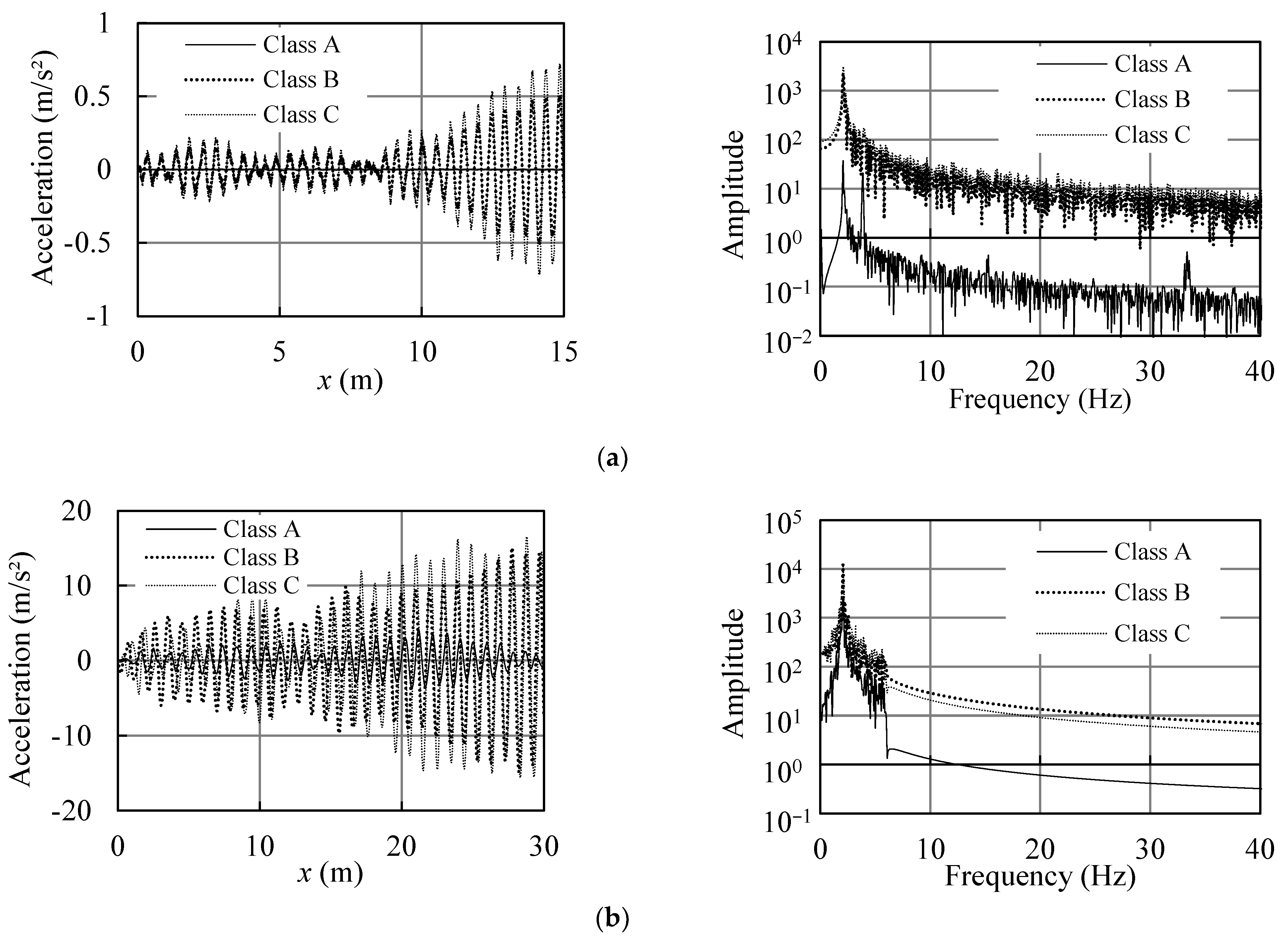
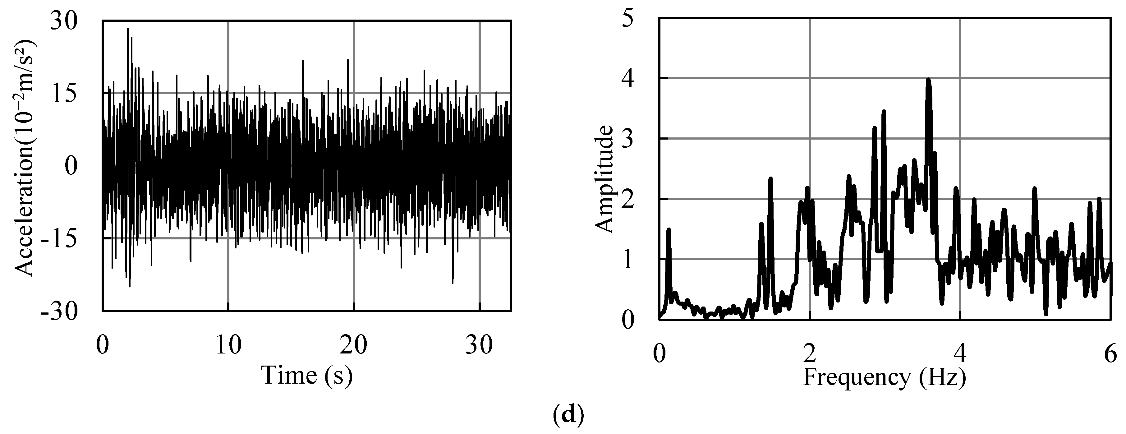
5.7.3. Influence of Vehicle Speed under Uneven Pavement Disturbances

Considering the influence of uneven pavement disturbances, the vehicle acceleration and its spectrogram at different speeds are shown in Figure 24. From the spectrogram, it can be observed that at low speed (v = 5 m/s), the fundamental frequency was relatively prominent, but the disturbances caused by the pavement were also evident and densely distributed. As the speed increased, the peak intervals in the spectrum became larger. In the high-speed states (v = 20 m/s and v = 30 m/s), the influence of pavement disturbances appeared to be relatively smaller, and the main issue causing difficulty in identification was the bifurcation of peaks. This phenomenon occurred because, as the speed increased, the time intervals between each time step became larger, or the vehicle covered a greater distance within the same time step. Thus, the road surface exhibited a smoother profile during high-speed travel. Due to the tire-enveloping characteristics of the vehicle, some short-wavelength components representing uneven pavement were masked, while these short-wavelength components in the road profile can generate significant acceleration responses for a point load. From this perspective, considering a vehicle as a point load under uneven pavement is an extreme assumption.

5.7.4. Influence of Vehicle Mass Uneven Pavement Disturbances

Using the two basic vehicle models mentioned, with a vehicle weight of m_v = 35,000 kg and stiffness k_v = 11,667 kN/m, and a vehicle weight of m_v = 1200 kg and stiffness k_v = 500 kN/m, three additional vehicles with weights of m_v = 25,000 kg, m_v = 15,000 kg, and m_v = 5000 kg were considered. The corresponding vehicle stiffness values were k_v = 8363 kN/m, k_v = 5059 kN/m, and k_v = 1755 kN/m, respectively. The road unevenness was classified as Grade A, and the velocity was v = 10 m/s.

The natural frequencies of the five vehicle models were 2.906 Hz, 2.911 Hz, 2.923 Hz, 2.982 Hz, and 3.249 Hz, respectively. Results of the vehicle acceleration signals under different vehicle models are shown in Figure 25. When the vehicle weight was larger, the disturbing forces caused by road unevenness were relatively smaller compared to the vehicle’s weight. In this case, the bridge vibrations primarily resulted from the gravitational effect of the vehicle. Therefore, increasing the vehicle weight appropriately can help in identifying the bridge frequencies. Another phenomenon observed was that the amplitude of the spectrum reached its maximum around 3 Hz. This is because the vehicle’s natural frequency was around 3 Hz, causing higher amplitude values in the vicinity of this frequency.

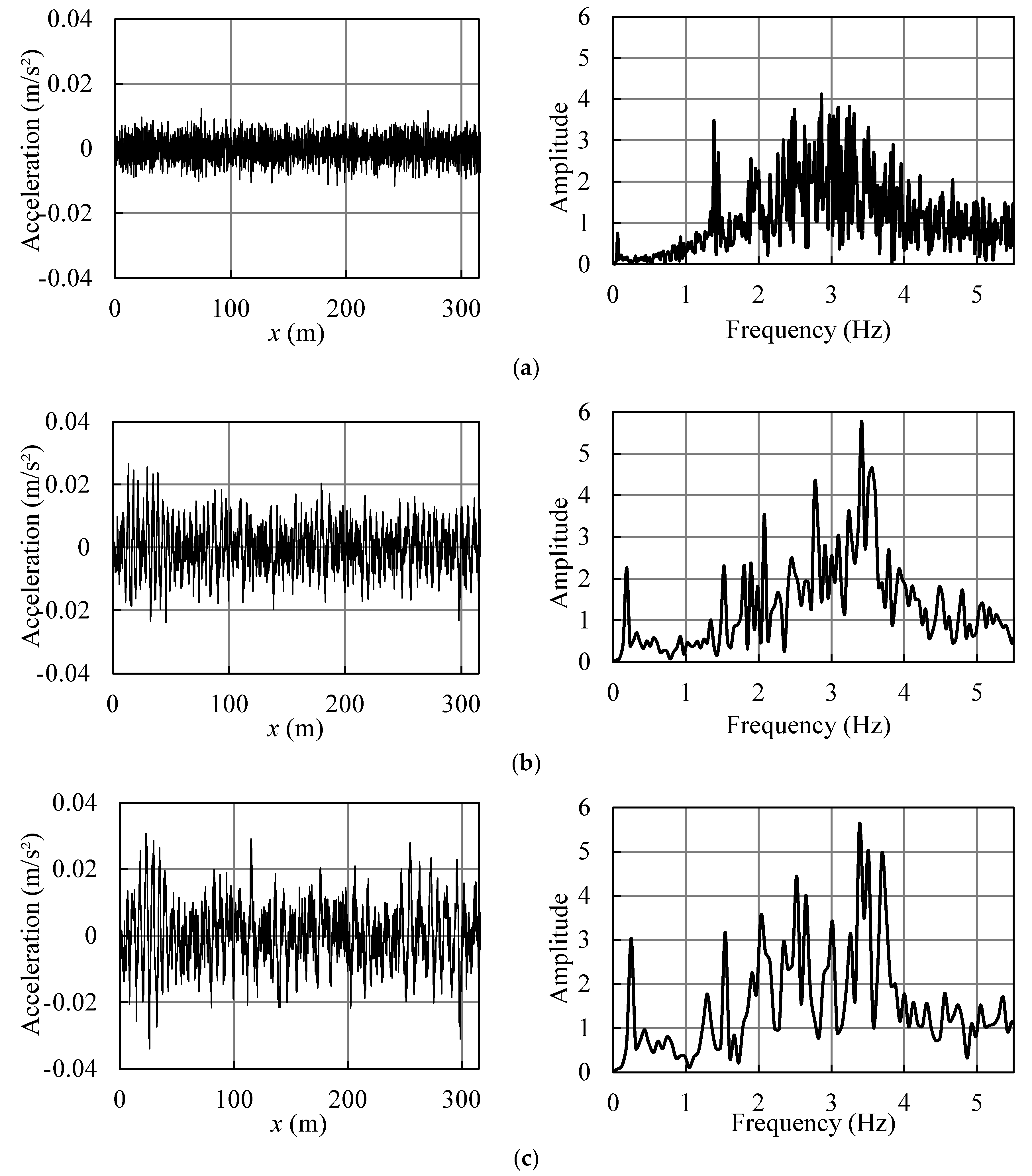
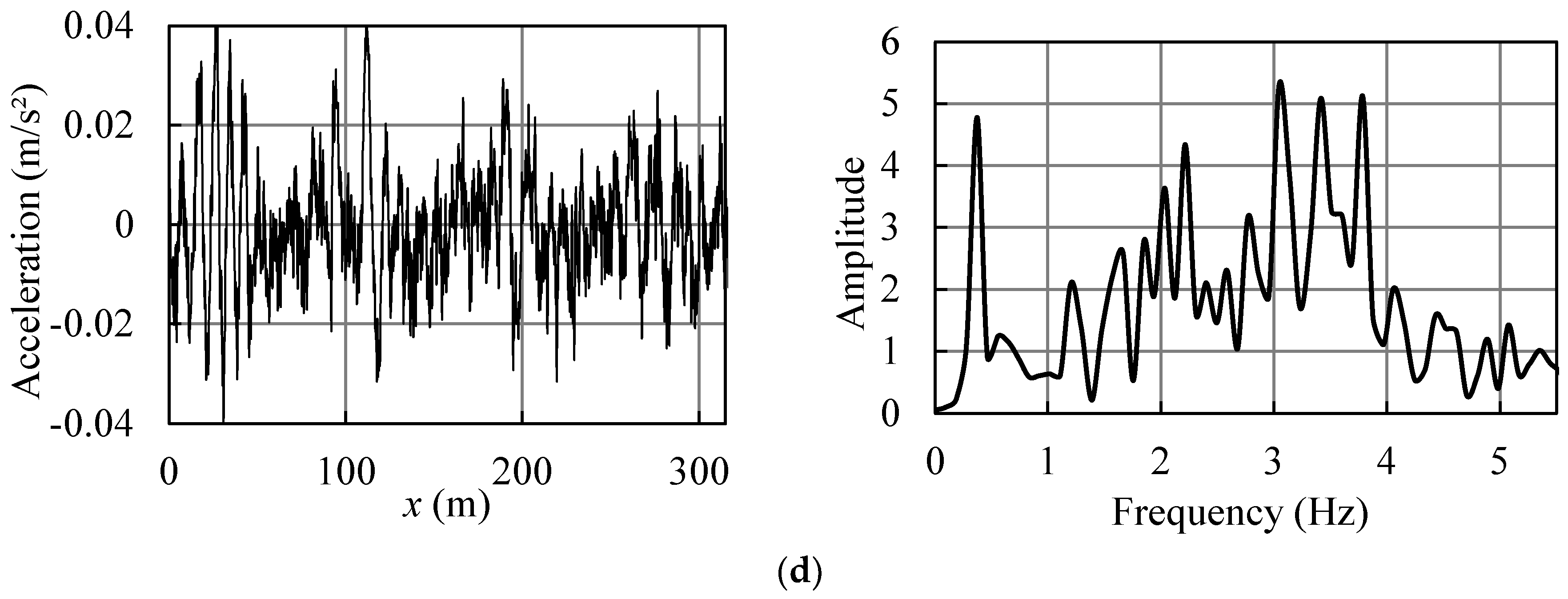
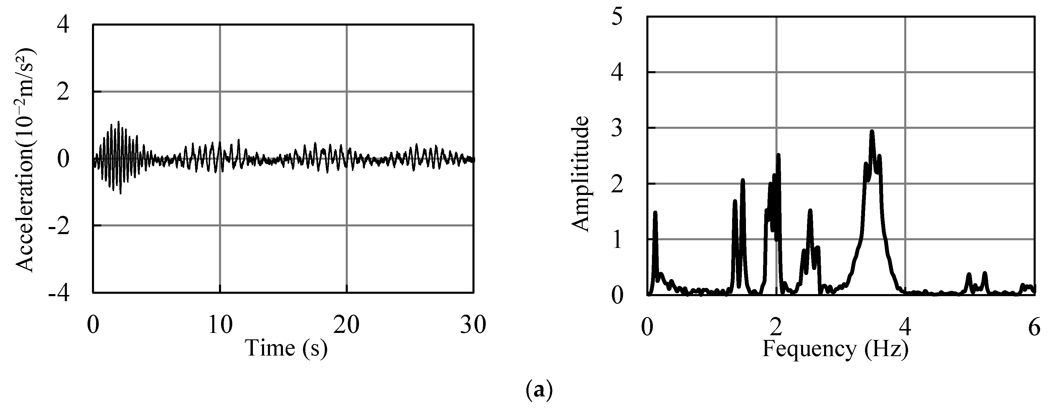
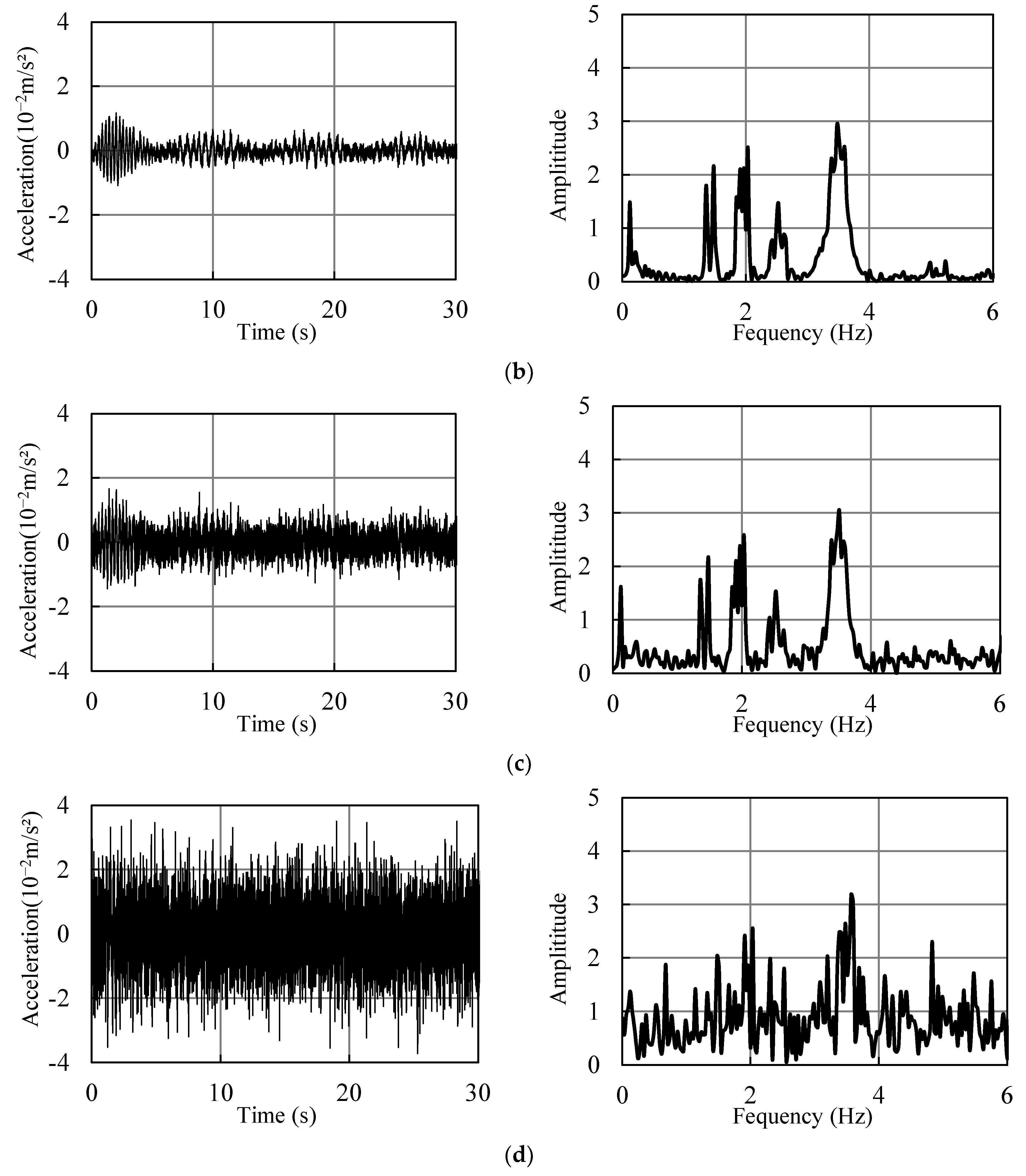
5.8. Influence of Interference Force

During vehicle operation, various factors, such as random vibrations of the vehicle body, can introduce interference forces. Although these forces are typically small, they can indeed exert an influence on frequency identification. To account for this effect, Gaussian white noise interference forces with specific power levels were considered. For the vehicle parameters mentioned before, including a speed of 10 m/s, weight of 350,000 kg, and stiffness of 11,667 kN/m, white noise interference forces with power levels of 20 dBW, 30 dBW, 40 dBW, and 50 dBW were applied. The corresponding standard deviations of these interference forces were 10 N, 31.6 N, 100 N, and 316.2 N, respectively.

The acceleration response and spectrum of the vehicles under different power levels are shown in Figure 26. As the power of the interference force increased, the amplitude of the interference frequency on the spectrum diagram gradually increased. When the power of the interference force reached 40 dBW (with a standard deviation of the interference force to vehicle gravity ratio at 0.029%), the influence of the interference force was relatively small. Beyond 40 dBW, the influence of the interference force became more significant, and only the fundamental frequency could be distinguished at 50 dBW.

5.9. Influence of Interference Signal

In the process of signal transmission, it is possible for the signals to be affected by electromagnetic environmental interference. The interference signals directly impact the signals themselves, resulting in disturbances. The distribution of these interference signals is similar to that of interference forces, as they appear randomly in time while maintaining a relatively stable power level. These interference signals can also be simulated using white noise signals. The original acceleration signal was based on the signal without interference forces applied. The time-domain and spectrogram of the vehicle acceleration under different signal-to-noise ratios (SNR) of the interference signals are shown in Figure 27. As the SNR gradually decreased, the power of the interference signals relative to the original signal increased, causing the original vibration signal of the vehicle to become increasingly blurred. When the interference signal became sufficiently strong, it completely masked the original vehicle vibration signal.

6. Conclusions

Based on the engineering background of the northern approach of Jiubao Bridge, a steel-concrete composite beam bridge, the feasibility of using the indirect method to measure the frequency of the composite beam bridge was analyzed. The influence of various parameters related to the composite beam bridge and the vehicle in the indirect method for measuring bridge frequencies was investigated, and the effects of factors such as road unevenness, interference forces, and interference signals were discussed. The main conclusions are as follows:

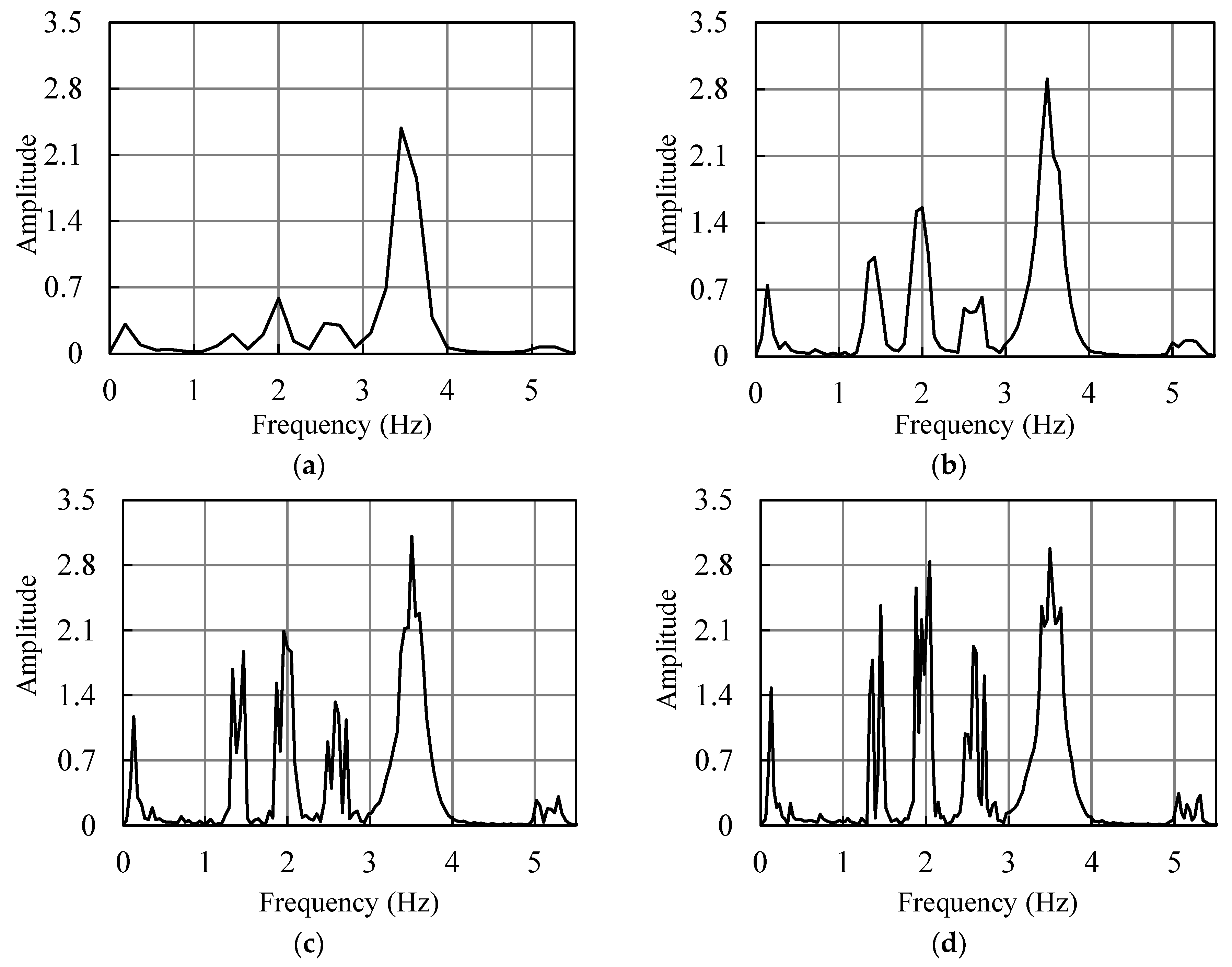
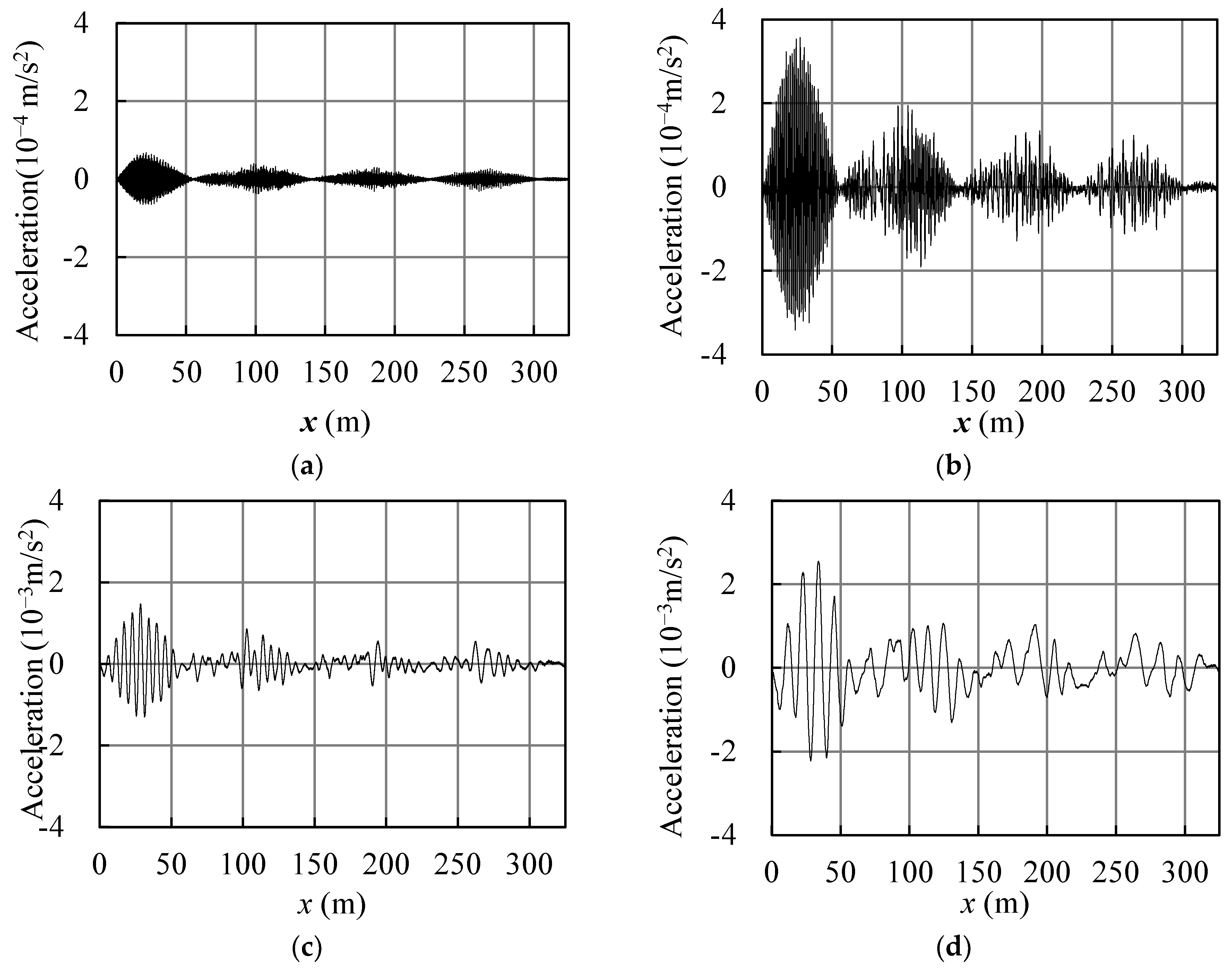
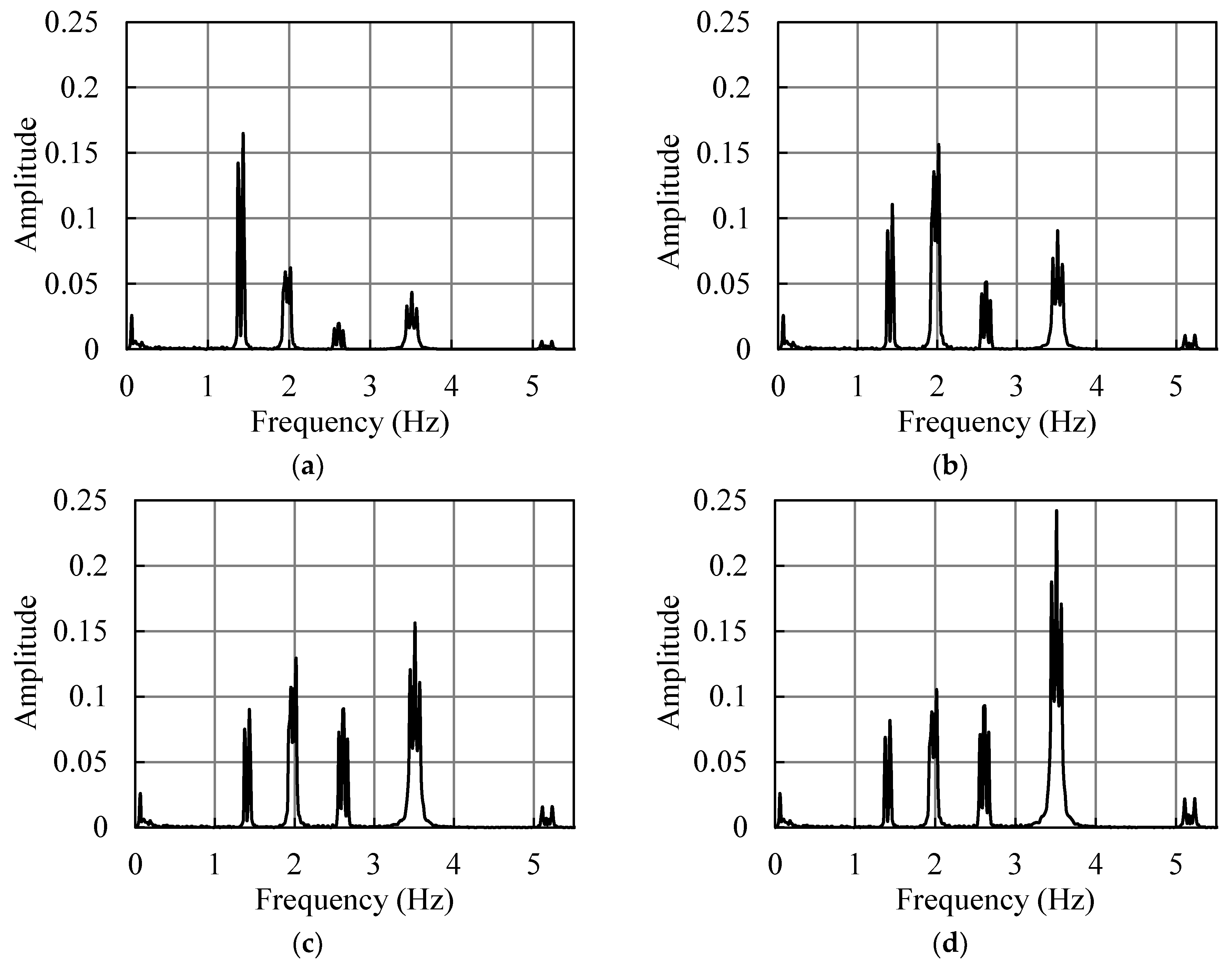
• In the ideal condition without interference, the indirect method exhibited a high level of accuracy in identifying the natural frequencies of the composite beam bridge, especially the fundamental frequency. In this ideal condition, the vehicle speed had a significant impact on the identification of the composite beam frequencies. Due to the influence of the vehicle’s driving frequency, the amplitude spectrum of the measured acceleration exhibited bifurcation peaks. Vehicle parameters also affected frequency identification, resulting in an increased amplitude around the vehicle’s natural frequency in the spectrogram. Vehicle damping, on the other hand, had a suppressing effect on the amplitude of all frequency orders. The interlayer shear stiffness of the composite beam and the magnitude of the prestress of the tendon can cause variations in the bridge frequency. The shear stiffness and the prestress value corresponding to fundamental frequencies after the changes can be identified using this method.
• The influence of road disturbances on frequency identification was such that the fundamental frequency can be identified when the road surface roughness is relatively low. Vehicles with larger masses contribute to improved frequency identification. As the vehicle speed increased, the amplitude of the acceleration spectrum also increased. However, the occurrence of bifurcation phenomena at the peak points became more pronounced, necessitating a comprehensive consideration when selecting an appropriate speed.

Due to limitations in research funding and time, the method proposed in this paper has not yet been applied to practical engineering projects. Research will be conducted in the next phase of our study, with the proposed method being applied to practical engineering practices.

References

1. Yang, Y.B.; Chang, K.C. Extraction of bridge frequencies from the dynamic response of a passing vehicle enhanced by the EMD technique. J. Sound Vib. 2009, 322, 718–739. [Google Scholar] [CrossRef]
2. Kim, J.T.; Stubbs, N. Crack detection in beam-type structures using frequency data. J. Sound Vib. 2003, 259, 145–160. [Google Scholar] [CrossRef]
3. Curadelli, R.O.; Riera, J.D.; Ambrosini, D.; Amani, M.G. Damage detection by means of structural damping identification. Eng. Struct. 2008, 30, 3497–3504. [Google Scholar] [CrossRef]
4. Kim, J.T.; Ryu, Y.S.; Cho, H.M.; Stubbs, N. Damage identification in beam-type structures: Frequency-based method vs mode-shape-based method. Eng. Struct. 2003, 25, 57–67. [Google Scholar] [CrossRef]
5. Chen, Q.; Wang, G. Computationally-efficient homogenization and localization of unidirectional piezoelectric composites with partially cracked interface. Compos. Struct. 2020, 232, 111452. [Google Scholar] [CrossRef]
6. Chen, Q.; Chen, W.; Wang, G. Fully-coupled electro-magneto-elastic behavior of unidirectional multiphased composites via finite-volume homogenization. Mech. Mater. 2021, 154, 103553. [Google Scholar] [CrossRef]
7. Carden, E.P.; Fanning, P. Vibration based condition monitoring: A review. Struct. Health Monit. Int. J. 2004, 3, 355–377. [Google Scholar] [CrossRef]
8. Alvandi, A.; Cremona, C. Assessment of vibration-based damage identification techniques. J. Sound Vib. 2006, 292, 179–202. [Google Scholar] [CrossRef]
9. Farrar, C.R.; Doebling, S.W.; Nix, D.A. Vibration-based structural damage identification. Philos. Trans. R. Soc. Lond. Ser. A-Math. Phys. Eng. Sci. 2001, 359, 131–149. [Google Scholar] [CrossRef]
10. Wu, R.; Xu, R.; Wang, G. Frequency domain homogenization of effective and localized viscoelastic response of unidirectional composites with imperfect interfaces. Compos. Struct. 2022, 301, 116226. [Google Scholar] [CrossRef]
11. Fang, S.-E.; Perera, R. Power mode shapes for early damage detection in linear structures. J. Sound Vib. 2009, 324, 40–56. [Google Scholar] [CrossRef]
12. Zhang, Y.; Wang, L.; Xiang, Z. Damage detection by mode shape squares extracted from a passing vehicle. J. Sound Vib. 2012, 331, 291–307. [Google Scholar] [CrossRef]
13. Yang, Y.B.; Lin, C.W.; Yau, J.D. Extracting bridge frequencies from the dynamic response of a passing vehicle. J. Sound Vib. 2004, 272, 471–493. [Google Scholar] [CrossRef]
14. Yang, Y.B.; Lin, C.W. Vehicle–bridge interaction dynamics and potential applications. J. Sound Vib. 2005, 284, 205–226. [Google Scholar] [CrossRef]
15. Yang, Y.B.; Chang, K.C.; Li, Y.C. Filtering techniques for extracting bridge frequencies from a test vehicle moving over the bridge. Eng. Struct. 2013, 48, 353–362. [Google Scholar] [CrossRef]
16. Malekjafarian, A.; Obrien, E.J. Identification of bridge mode shapes using Short Time Frequency Domain Decomposition of the responses measured in a passing vehicle. Eng. Struct. 2014, 81, 386–397. [Google Scholar] [CrossRef]
17. McGetrick, P.J.; Gonzalez, A.; Obrien, E.J. Theoretical investigation of the use of a moving vehicle to identify bridge dynamic parameters. Insight 2009, 51, 433–438. [Google Scholar] [CrossRef]
18. Pesterev, A.V.; Yang, B.; Bergman, L.A.; Tan, C.A. Response of elastic continuum carrying multiple moving oscillators. J. Eng. Mech.-ASCE 2001, 127, 260–265. [Google Scholar] [CrossRef]
19. Yang, Y.B.; Wu, Y.S. A versatile element for analyzing vehicle-bridge interaction response. Eng. Struct. 2001, 23, 452–469. [Google Scholar] [CrossRef]
20. Xia, H.; Xu, Y.L.; Chan, T.H.T. Dynamic interaction of long suspension bridges with running trains. J. Sound Vib. 2000, 237, 263–280. [Google Scholar] [CrossRef]
21. Yang, Y.B.; Chang, C.H.; Yau, J.D. An element for analysing vehicle-bridge systems considering vehicle’s pitching effect. Int. J. Numer. Methods Eng. 1999, 46, 1031–1047. [Google Scholar] [CrossRef]
22. Zhang, L.; Xu, Z.; Gao, M.; Xu, R.; Wang, G. Static, dynamic and buckling responses of random functionally graded beams reinforced by graphene platelets. Eng. Struct. 2023, 291, 116476. [Google Scholar] [CrossRef]
23. Wu, R.; Xu, R.; Wang, G. Multiscale viscoelastic analysis of FRP-strengthened concrete beams. Int. J. Mech. Sci. 2023, 253, 108396. [Google Scholar] [CrossRef]
24. Wu, R.; Xu, R.; Wang, G. Modeling and prediction of short/long term mechanical behavior of FRP-strengthened slabs using innovative composite finite elements. Eng. Struct. 2023, 281, 115727. [Google Scholar] [CrossRef]
25. Lin, J.-P.; Wang, G.; Bao, G.; Xu, R. Stiffness matrix for the analysis and design of partial-interaction composite beams. Constr. Build. Mater. 2017, 156, 761–772. [Google Scholar] [CrossRef]
26. Lin, J.-P.; Wang, G.; Xu, R. Variational Principles and Explicit Finite-Element Formulations for the Dynamic Analysis of Partial-Interaction Composite Beams. J. Eng. Mech. 2020, 146, 04020055. [Google Scholar] [CrossRef]
27. Pan, J. Vehicle-Bridge Interaction Analysis by the Symplectic Method. Master’s Thesis, Zhejiang University, Hangzhou, China, 2014. [Google Scholar]
28. ISO 8608; Mechanical Vibration-Road Surface Profiles-Reporting of Measured Data. International Standardization Organization: Geneva, Switzerland, 2006.
29. Yang, Y.B.; Li, Y.C.; Chang, K.C. Effect of road surface roughness on the response of a moving vehicle for identification of bridge frequencies. Interact. Multiscale Mech. 2012, 5, 347–368. [Google Scholar] [CrossRef]
30. Chen, X. The Vehicle-Bridge Interaction Analysis of Corrugated Steel Web Box Girder Based on Contact-Constraint Method. Master’s Thesis, Chongqing University, Chongqing, China, 2019. [Google Scholar]
Figure 1. The coordinates of the e-th element.
Applsci 13 12534 g001
Figure 2. A partial interaction composite beam with a moving mass-spring-damper system.
Applsci 13 12534 g002
Figure 3. (a) Vertical dynamic mid-span velocity, (b) vertical dynamic vehicle velocity, (c) vertical dynamic mid-span acceleration, (d) vertical dynamic vehicle acceleration, and (e) vertical dynamic vehicle displacements.
Applsci 13 12534 g003aApplsci 13 12534 g003b
Figure 4. The span layout of Jiubao Bridge (m) and the standard section of the northern approach bridge (unit: cm). (a) Span layout; (b) standard section.
Applsci 13 12534 g004
Figure 5. Dynamic response of the bridge at the middle of the second span. (a) Vertical displacement; (b) vertical displacement spectrum; (c) acceleration; (d) acceleration spectrum.
Applsci 13 12534 g005
Figure 6. Dynamic response of the vehicle. (a) Vertical displacement; (b) vertical displacement spectrum; (c) acceleration; (d) acceleration spectrum.
Applsci 13 12534 g006
Figure 7. The first 4 mode shapes of the deflection for the northern approach bridges.
Applsci 13 12534 g007
Figure 8. Acceleration spectrum of the vehicle with different vehicle running times: (a) 1 span (t = 5.5 s); (b) 2 span (t = 14.0 s); (c) 3 span (t = 22.5 s); (d) 4 span (t = 30.3 s).
Applsci 13 12534 g008
Figure 9. The influence of the moving speed of the vehicle on acceleration: (a) v = 1 m/s; (b) v = 5 m/s; (c) v = 20 m/s; (d) v = 40 m/s.
Applsci 13 12534 g009
Figure 10. The influence of the moving speed of the vehicle on the acceleration spectrum: (a) v = 1 m/s; (b) v = 5 m/s; (c) v = 20 m/s; (d) v = 40 m/s.
Applsci 13 12534 g010
Figure 11. The influence of vehicle moving speed on the acceleration of vehicle. (a) Maximum acceleration; (b) maximum amplitude of acceleration spectrum.
Applsci 13 12534 g011
Figure 12. The influence of vehicle moving speed on the maximum acceleration and maximum deflection of the bridge at the middle of the second span. (a) Acceleration; (b) deflection.
Applsci 13 12534 g012
Figure 13. The influence of vehicle stiffness on the acceleration spectrum: (a) kv = 100 kN/m; (b) kv = 200 kN/m; (c) kv = 300 kN/m; (d) kv = 400 kN/m.
Applsci 13 12534 g013
Figure 14. The influence of the vehicle damping ratio on the acceleration spectrum: (a) ξv = 0.02; (b) ξv = 0.1; (c) ξv = 0.4; (d) ξv = 0.8.
Applsci 13 12534 g014
Figure 15. The influence of vehicle mass on the acceleration spectrum: (a) mv = 1.5 ton; (b) mv = 2.0 ton; (c) mv = 2.5 ton; (d) mv = 3.0 ton.
Applsci 13 12534 g015
Figure 16. The influence of shear stiffness on the acceleration spectrum: (a) ks = 10 MPa; (b) ks = 100 MPa; (c) ks = 1000 MPa; (d) ks = 10,000 MPa.
Applsci 13 12534 g016
Figure 17. The influence of the prestress of the tendon on the acceleration spectrum: (a) f = 100 kN; (b) f = 10,000 kN; (c) f = 1,000,000 kN; (d) f = 1,600,000 kN.
Applsci 13 12534 g017
Figure 18. The prestress–frequency curve obtained from free vibration analysis.
Applsci 13 12534 g018
Figure 19. Road surface profile generated: (a) Model 1, (b) Model 2, and (c) Model 3.
Applsci 13 12534 g019
Figure 20. Acceleration under smooth pavement.
Applsci 13 12534 g020
Figure 21. The time–domain acceleration curve and the acceleration spectrum: (a) Model 1, (b) Model 2, and (c) Model 3.
Applsci 13 12534 g021aApplsci 13 12534 g021b
Figure 22. Road surface profile generated.
Applsci 13 12534 g022
Figure 23. Acceleration and frequency responses of the test vehicle at different pavement grades for (a) Grade A, (b) Grade B, and (c) Grade C.
Applsci 13 12534 g023
Figure 24. Acceleration and frequency responses of the test vehicle at different vehicle speeds: (a) v = 5 m/s; (b) v = 15 m/s; (c) v = 20 m/s; (d) v = 30 m/s.
Applsci 13 12534 g024aApplsci 13 12534 g024b
Figure 25. Acceleration and frequency responses of the test vehicle at different vehicle masses: (a) mv = 1200 kg; (b) mv = 5000 kg; (c) mv = 15,000 kg; (d) mv = 25,000 kg.
Applsci 13 12534 g025aApplsci 13 12534 g025b
Figure 26. Acceleration and frequency responses of the test vehicle at different interference power values: (a) 20 dBW; (b) 30 dBW; (c) 40 dBW; (d) 50 dBW.
Applsci 13 12534 g026aApplsci 13 12534 g026b
Figure 27. Acceleration and frequency responses of the test vehicle at different SNRs: (a) SNR = 70 dB; (b) SNR = 60 dB; (c) SNR = 50 dB; (d) SNR = 40 dB.
Applsci 13 12534 g027aApplsci 13 12534 g027b