RPREC: A Radar Plot Recognition Algorithm Based on Adaptive Evidence Classification

Abstract

When radar receives target echoes to form plots, it is inevitably affected by clutter, which brings a lot of imprecise and uncertain information to target recognition. Traditional radar plot recognition algorithms often have poor performance in dealing with imprecise and uncertain information. To solve this problem, a radar plot recognition algorithm based on adaptive evidence classification (RPREC) is proposed in this paper. The RPREC can be considered as the evidence classification version under the belief functions. First, the recognition framework based on the belief functions for target, clutter, and uncertainty is created, and a deep neural network model classifier that can give the class of radar plots is also designed. Secondly, according to the classification results of each iteration round, the decision pieces of evidence are constructed and fused. Before being fused, evidence will be corrected based on the distribution of radar plots. Finally, based on the global fusion results, the class labels of all radar plots are updated, and the classifier is retrained and updated so as to iterate until all the class labels of radar plots are no longer changed. The performance of the RPREC is verified and analyzed based on the real radar plot datasets by comparison with other related methods.

1. Introduction

Due to the influence of detection accuracy and clutter, radars will form a large number of clutter plots when receiving target echoes for processing, which is not conducive to target recognition. Especially in areas with high-clutter density, the target plots can hardly be seen [1,2]. In order to eliminate radar detection errors, multiple radars will work together. But at this point, they can also cause clutter plots to overlap with each other, forming a dense clutter area with irregular spatial distribution, seriously affecting the recognition accuracy and real-time performance of radar data processing. It can be seen that in radar plot processing, how to effectively detect targets from a large amount of clutter and uncertain plots is the key to achieving precise target tracking by radar [3,4,5]. In order to ensure efficient and fast data processing for radar plots, traditional radar plot recognition algorithms usually use binary classification recognition rules to determine whether they are a target or clutter [6,7,8,9]. However, it is well-known that targets cannot be accurately classified in some cases. Therefore, due to the inability to effectively represent the uncertain measurements, this yes or no decision judgment can increase the error rate. This is not conducive to correct decision analysis in these traditional methods. There are two main ways to solve this problem: one is to use belief functions to accurately represent uncertain information, and the other is to use deep neural networks with stronger sample learning ability for classification. The belief functions have significant advantages in dealing with uncertain and imprecise information [10,11,12,13,14]. So, they have been applied in some fields such as pattern recognition [15,16], data clustering [17,18,19,20,21,22,23], data classification [16,24,25,26,27], security assessment [28,29], sensor information fusion [30], abnormal detection [31], tumor segmentation [32,33], decision-making [34,35,36], community detection [37,38], and items of interest recommendation [39,40]. Considering the good performance of belief functions in application, evidence classification algorithms have been studied to improve the accuracy of target recognition. Among these methods, the evidence K-nearest neighbor (EK-NN) is the most representative [25,41]. Subsequently, in order to adapt to different application scenarios, some modifications of the EK-NN have been studied. For instance, many optimization methods based on the EK-NN were proposed in [42,43,44,45]. Generally, these improved algorithms can have good performances in some domains, such as machine diagnosis [46], process control [47], remote sensing [48], medical image processing [49], and bioinformatics [50,51], among others.

Compared with traditional classification methods, the deep neural network model has strong learning ability and also the advantage of constantly updating with an increase in samples [52,53,54,55,56]. Therefore, radar plot recognition algorithms based on neural networks have been studied. In reference [53], the full connected neural network (FNN) is used to study the classification of radar clutter and real targets. The authors designed a network with five layers, with nodes in each layer being 8, 64, 128, 32, and 2. When the number of training and testing samples is 6276 and 2000, respectively, the classification accuracy of the FNN can reach approximately 0.83 to 0.88. In reference [54], a multi-layer perceptron algorithm optimized by particle swam optimization was used for radar plot recognition (PSO-MLP), which achieved a good recognition accuracy of 0.857. In reference [55], the convolutional neural network (CNN) was compared with the fully connected neural network (FNN) and support vector machine (SVM). The experimental results show that when the training and testing samples are sufficient, the recognition accuracy of the CNN can reach 0.943. In reference [56], the same authors used the recurrent neural network (RNN) instead of the CNN to further improve classification accuracy. When the training samples of radar plots exceed 10000, the recognition accuracy can reach 0.991, which is impressive.

Therefore, in order to effectively characterize the uncertain data and also improve the recognition accuracy, a radar plot recognition algorithm based on adaptive evidence classification (RPREC) is proposed in this paper. In the RPREC, a confidence recognition framework is first created that includes target, clutter, and uncertainty, and an updatable classifier based on deep neural networks is also designed. Then, based on the network classification model obtained in each round, the category of all radar plots can be confirmed. If the network classification model does not have samples for training, the class of each radar plot will be randomly initially given. Finally, the class of each radar plot is updated through the fusion of belief functions, and the plots after updating the category label can be used for classifier training and parameter optimization. The optimized classifier can also be reused to obtain the class of each plot. This cycle continues until the category labels of each plot are no longer updated or iterated to a certain number. The performance of the RPREC is verified through some experiments based on the real radar plot dataset. The results show that the RPREC can effectively handle clutter and uncertain data compared to other typical algorithms. So, it can improve the recognition accuracy of radar plots. In addition, the RPREC has less dependence on training samples, making it easy to apply to other scenarios.

The rest of this paper is organized as follows. In Section 2, we will recall the belief functions and the evidence K-nearest neighbor classification, respectively. In Section 3, we will introduce the proposed radar plot recognition algorithm based on adaptive evidence classification. Finally, experiments will be presented in Section 4, and the paper will be concluded in Section 5.

2. Related Work

Firstly, the belief function theory is introduced in Section 2.1. Then, the K-nearest neighbor classification of evidence was reviewed in Section 2.2.

2.1. Belief Functions

The belief functions can be seen as a generalization of probability theory. They have been proven to be an effective theoretical framework, especially in the processing of uncertain and imprecise information.

In belief functions, the set $\Omega =\{{\omega }_1,\cdots ,{\omega }_c\}$ is called discernment, which can be extended to the powerset $2^{\Omega }$. For example, if $\Omega =\{{\omega }_1,{\omega }_2,{\omega }_3\}$, then $2^{\Omega }=\{\varnothing ,\{{\omega }_1\},\{{\omega }_2\},\{{\omega }_3\},\{{\omega }_1,{\omega }_2\},\{{\omega }_1,{\omega }_3\},\{{\omega }_2,{\omega }_3\},\Omega \}$. The mass function m is used to express the belief of the different elements in $2^{\Omega }$, which is a mapping function from $2^{\Omega }$ to the interval [0, 1] that is defined by:

$$m(\varnothing )=0,{\displaystyle \sum _{A\subseteq 2^{\Omega },A\ne \varnothing }m(A)}=1$$

(1)

Subsets $A\in 2^{\Omega }$ are called the focal sets that satisfy $m(A)>0$. Each number m (A) is interpreted as the probability that the evidence supports exactly the assertion A. In particular, m (Ω) is the probability that the evidence tells us nothing about ω, i.e., it is the probability of knowing nothing. For any subset $A\in 2^{\Omega }$, the probability that the evidence supports A and the probability that the evidence does not contradict A can be defined as:

$$Bel(A)={\displaystyle \sum _{B\subseteq A}m(B)}$$

(2)

$$Pl(A)={\displaystyle \sum _{B\cap A\ne \varnothing }m(B)}.$$

(3)

Functions Bel and Pl are called, respectively, the belief function and the plausibility function associated with m. They can be regarded as providing lower and upper bounds for the degree of belief that can be attached to each subset of Ω.

In the Dempster–Shafer (D-S) theory, independent evidence can be combined with each other to ultimately form the belief that supports decision-making. Assume that on the same frame of discernment, there are two pieces of evidence represented by m₁ and m₂, respectively. Then, the evidence combination based on the D-S rule is defined as:

$$(m_1\oplus m_2)(A)=\frac{{\displaystyle \sum _{B\cap C=A}{m}_1(B)m_2}(C)}{1-k}$$

(4)

And:

$$k={\displaystyle \sum _{B\cap C=\varnothing }{m}_1(B)m_2}(C)$$

(5)

k is used to represent the degree of conflict between evidence, where the evidence refers to m₁ and m₂. If k = 0, these two pieces of evidence are completely consistent and there is no conflict between them. If k = 1, these two pieces of evidence are completely contradictory and cannot be combined.

For example, let us consider $\Omega =\{{\omega }_1,{\omega }_2\}$ and the two pieces of evidence providing the following mass function:

$$\begin{array}{c}{m}_1({\omega }_1)=0.8, m_1({\omega }_2)=0.2\\ m_2({\omega }_1)=0.7, m_2({\omega }_2)=0.3\end{array}$$

Using the D-S rule to combine these two pieces of evidence, one obtains:

$$\begin{array}{c}{m}_{DS}({\omega }_1)=m_1({\omega }_1)m_2({\omega }_1)=0.56\\ m_{DS}({\omega }_2)=m_1({\omega }_2)m_2({\omega }_2)=0.06\\ m_{DS}({\omega }_1\cap {\omega }_2)=m_1({\omega }_1)m_2({\omega }_2)+m_1({\omega }_2)m_2({\omega }_1)=0.38\end{array}$$

Here, $K=m_{DS}({\omega }_1\cap {\omega }_2)=0.38$ is the degree of conflict between m₁ and m₂.

The two pieces of evidence provide the following mass function:

$$\begin{array}{c}{m}_1({\omega }_1)=1, m_1({\omega }_2)=0\\ m_2({\omega }_1)=0, m_2({\omega }_2)=1\end{array}$$

Combining these two pieces of evidence with the D-S rule, one obtains:

$$m_{DS}({\omega }_1)=0, m_{DS}({\omega }_2)=0, m_{DS}({\omega }_1\cap {\omega }_2)=1$$

Then, $K=m_{DS}({\omega }_1\cap {\omega }_2)=1$. The fusion result is meaningless because of the full contradiction of the two sources of information. Therefore, when the degree of conflict is very high, the two pieces of evidence cannot be combined.

2.2. Evidence Classification

In the design of evidence classification algorithms based on belief function frameworks, the evidential K-nearest neighbor classification (EK-NN) plays a significant role. In the EK-NN, each neighbor of the sample is considered as evidence, which is used to provide decision support for the class label of the sample. The final decision is presented by combining these K-nearest neighbor pieces of evidence.

Consider a data classification problem where the object $o$ will be classified into a certain class that belongs to the class set $\Omega =\{{\omega }_1,\cdots ,{\omega }_c\}$. If the nearest neighbor $o_j$ with a feature distance of $d_j$ from the target $o$ belongs to the group ${\omega }_{k(j)}$, then the evidence of each neighbor can be represented by the following formula.

$$\left\{\begin{array}{c}{m}_j(\{{\omega }_{k(j)}\})=\phi (d_j)\\ m_j(\Omega )=1-\phi (d_j)\end{array}\right.$$

(6)

where φ is a non-increasing mapping from [0, +∞) to [0, 1], and it was proposed to choose φ as:

$$\phi (d_j)={\alpha }_0\exp (-{\gamma }_q{d}_j)$$

(7)

The set of these nearest neighbors is represented by N_K; therefore, the combination of the mass function of the nearest neighbors becomes:

$$m=\underset{j\in N_k}{{\displaystyle \oplus }} m_j.$$

(8)

At this point, the final decision can be made that object is assigned to the class ${\omega }_q$ with the highest confidence level. The EK-NN provides a good idea for data classification with uncertain information.

In order to present the characteristics of evidence classification more intuitively and clearly, the flowchart of evidence classification is shown below in Figure 1:

3. Proposed Method

In this section, the radar plot recognition algorithm based on adaptive evidence classification (RPREC) is presented in detail. The RPREC mainly includes three parts. In Section 3.1, the confidence recognition framework for target, clutter, and uncertainty has been constructed, and a deep neural network classification model has also been designed. In Section 3.2, the mass function of each radar plot was constructed, and the evidence was corrected and fused. In Section 3.3, iterative updating of category labels for target data was carried out based on the real-time optimization of classifiers.

3.1. Design of a Neural Network Classifier

In the RPREC, the recognition framework $\Omega =\{C_o,C_n,\Theta \}$ for target, clutter, and uncertainty plots is first constructed, which is different from the binary recognition rule of either target or clutter in traditional methods. Here, $C_o$ represents the category of the real target plots, $C_n$ represents the category of clutter, and $\Theta$ represents the category of uncertainty. The mathematical relationship between them is: $C_o\cap C_n=\varnothing$, $C_o\cap \Theta =C_o$, and $C_n\cap \Theta =C_n$.

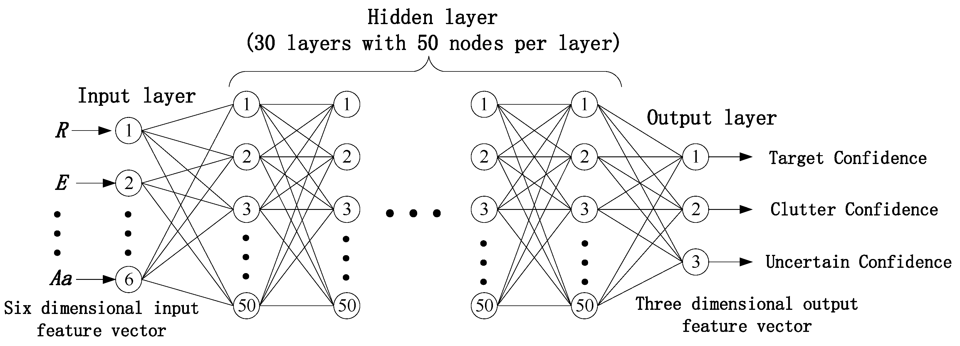
As shown in Figure 2, a fully connected neural network has been designed, which can continuously optimize as the confidence function of the plots’ category is iteratively updated. The specific network parameters are set as follows:

Input layer: The network input is the collected radar plot data, including target, clutter, and uncertainty. Before being input into the network classifier for category recognition, all plots are modeled using feature vectors recommended in [53]. The mathematical representation is $F=[R,E,Rw,Aw,Ma,Aa]$. Here, R represents the distance from the target to the radar, E represents the altitude information, Rw represents the size of the target in the distance, Aw represents the size of the target in the azimuth, Ma represents the maximum amplitude of all participating condensation echoes, and Ma represents the average amplitude of all participating condensation echoes.

Therefore, the number of nodes in this network input layer is set to 6, which is consistent with the input feature dimension.

Output layer: The network output represents the category membership of plots belonging to $C_o$, $C_n$, and $\Theta$ under the confidence recognition framework $\Omega$. It represents the confidence level of radar plots belonging to target, clutter, and uncertainty, respectively. Its mathematical representation is $\mu =[{\mu }_{C_o},{\mu }_{C_n},{\mu }_{\Theta }]$; therefore, the number of output nodes is set to 3.

Hidden layer: The design of network hidden layers is usually related to the size and distribution characteristics of the dataset. After some preliminary experiments, setting the hidden layer to 30 layers with 50 nodes per layer and using the sigmoid function for nonlinear processing has the best effect.

3.2. Construction and Correction Fusion of Belief Functions

The belief function is often referred to as the mass function. The construction and fusion of the mass function for the target plot mainly include three parts: initial classification of target data, construction of mass function, and correction and combination of evidence.

3.2.1. Initial Classification of Radar Plots

For the radar plots dataset $O=\{o_1,\cdots ,o_n\}$, based on the constructed deep network model classifier under the confidence recognition framework $\Omega =\{C_o,C_n,\Theta \}$, the category membership of target $O_i$$(i=1,\cdots ,n)$ can be obtained as ${\mu }_i=({\mu }_{i1},\cdots ,{\mu }_{ic})$, which satisfies the following equations:

$${\mu }_{ij}\in [0,1], {\displaystyle \sum _{j=1}^c{\mu }_{ij}}=1$$

(9)

Due to the limitations of the framework Ω, the value of category C is taken as 3, representing the target, clutter, and uncertainty, respectively. The number of radar plots belonging to classes $C_o$, $C_n$, and $\Theta$ is separately counted as $N_1$, $N_2$, and $N_3$. The total belief of each category is defined as:

$$\left\{\begin{array}{l}Bel(C_o)={\displaystyle \sum _{i=1}^{N_1}{\mu }_i(C_o)}\hfill \\ Bel(C_n)={\displaystyle \sum _{i=1}^{N_2}{\mu }_i(C_n)}\hfill \\ Bel(\Theta )={\displaystyle \sum _{i=1}^{N_3}{\mu }_i(\Theta )}\hfill \end{array}\right.$$

(10)

Here, the total belief can be seen as a description of the confidence density of radar plots in various categories. The sample data around the target can be used as auxiliary evidence for category decision-making, among which samples belonging to the same category can be used for confidence enhancement, while heterogeneous samples can be used for confidence correction. Therefore, a certain number of nearest neighbor samples can be selected from the three types of target plots formed by the above initial classification to construct decision evidence.

3.2.2. Construction of Mass Function

The samples were selected separately from the sample sets of categories $C_o$, $C_n$, and $\Theta$, with specific numerical settings proportional to the total belief, as shown in the following formula:

$$K_i=\frac{Bel(i)\times K}{{\displaystyle \sum _{i\in \{C_o,C_n,\Theta \}}Bel(i)}}$$

(11)

where the value of K is related to the size and distribution of radar plots and needs to be obtained through specific experiments based on different application backgrounds. After obtaining the nearest neighbor samples of the target point, the decision evidence set ${\Phi }_K(i)$ of target $o_i$ can be constructed. The basic confidence assignment function for each sample in this set is defined as:

$$\left\{\begin{array}{l}{m}_i(C_j)={\alpha }_{ij}\hfill \\ m_i(\Theta )=1-{\alpha }_{ij}\hfill \end{array},j=1,\cdots ,\right.K$$

(12)

With:

$${\alpha }_{ij}=\left\{\begin{array}{l}\lambda e^{-M_{ij}} , C_j\in \{C_o,C_n\}\hfill \\ 0 , C_j=\Theta \hfill \end{array}\right.$$

(13)

where $M_{ij}$ is the confidence similarity between the target data and the decision sample, defined as:

$$M_{ij}=\sqrt{{\displaystyle \sum _{c_i,c_j\in \left\{c_0,c_n,\Theta \right\}}(}Be{l}_i(C_i)-Be{l}_j(C_j){)}^2}$$

(14)

3.2.3. Correction and Combination of Evidence

This section mainly focuses on revising and combining decision evidence. Firstly, the evidence belonging to the same category is combined, and then the combination results belonging to different categories are fused.

1.

Combining evidence with the same category

Firstly, combine the evidence with the same category assignment in decision evidence set ${\Phi }_K(i)$; that is, combine the evidence in the decision evidence subset $T_q$ of each category.

$$\left\{\begin{array}{l}{m}_t^{T_q}(C_q)=1-{\displaystyle \prod _{j\in T_q}{m}_{i,j}(\Theta )}\hfill \\ m_t^{T_q}(\Theta )={\displaystyle \prod _{j\in T_q}{m}_{i,j}(\Theta )}\hfill \end{array}\right.$$

(15)

Assuming that $E_{\mathrm{r}}$ is the error rate of the radar plot, the setting of the evidence discount factor is defined as:

$$W_{C_q}=\frac{(1-E_{\mathrm{r}})\times Bel(C_q)}{{\displaystyle \sum _{C_q\in \{C_o,C_n,\Theta \}}Bel(C_q)}}$$

(16)

Based on the correction factor, the update of evidence can be achieved as follows:

$$\left\{\begin{array}{l}d{m}_t^{T_q}(C_q)=W_{C_q}(1-{\displaystyle \prod _{j\in T_q}{m}_{t,j}(\Theta ))}\hfill \\ d{m}_t^{T_q}(\Theta )=1-W_{C_q}(1-{\displaystyle \prod _{j\in T_q}{m}_{t,j}(\Theta ))}\hfill \end{array}\right.$$

(17)

2.

Combining the results under different categories

There may be certain confidence conflicts between different categories of decision evidence. The definition of evidence conflict between different categories is as follows:

$$T_c={\displaystyle \sum _{q=1}^{c}d{m}_t^{T_q}({\omega }_q)}$$

(18)

Therefore, for the initial fusion evidence $d{m}_t^{T_q}$ of different categories $T_q$, a combination based on conflict resolution rules can be obtained as follows:

$$\left\{\begin{array}{l}{m}_t(C_q)=(d{m}_t^{T_q}(C_q){\displaystyle \prod _{h\in \{1,\cdots ,c\},h\ne q}d{m}_t^{T_h}(\Theta ))/(1-T_c)}\hfill \\ m_t(\Theta )=1-{\displaystyle \sum _{q=1}^c(d{m}_t^{T_q}({\omega }_q){\displaystyle \prod _{h\in \{1,\cdots ,c\},h\ne q}d{m}_t^{T_h}(\Theta )})/(1-T_c)}\hfill \end{array}\right.$$

(19)

Here, $m_t$ is the global mass function obtained from the fusion of decision evidence set ${\Phi }_K(i)$. Then, the confidence level $Bel$ and the probability level $Pl$ of target $o_i$ belonging to each pattern category $C_i$ can be calculated.

$$Be{l}_i(C_i)={\displaystyle \sum _{C_i\in \{C_o,C_n,\Theta \},C_q\subseteq C_i}{m}_t(C_q)}$$

(20)

$$P{l}_i(C_i)={\displaystyle \sum _{C_i\in \{C_o,C_n,\Theta \},C_q\cap C_o\ne \varnothing }{m}_t(C_q)}$$

(21)

The criteria for updating the category labels of radar plots are:

Criterion 1: Update categories with maximum confidence;

Criterion 2: The minimum confidence difference between the new category and other categories must be greater than the threshold T1, which means that there must be sufficient confidence differences between different categories;

Criterion 3: The difference between the probability and confidence of the updated category must be less than the threshold T2, which means that the uncertainty of the category cannot be too high.

For example, let us assume that there are four pieces of evidence in the decision evidence set ${\Phi }_K(i)$:

$$\begin{array}{c}{m}_1(C_o)=0.8, m_1(\Theta )=0.2\\ m_2(C_o)=0.7, m_2(\Theta )=0.3\\ m_3(C_n)=0.8, m_3(\Theta )=0.2\\ m_4(C_n)=0.6, m_3(\Theta )=0.4\end{array}$$

Firstly, combine the evidence with the same category. That is, evidence 1 and 2 need to be combined, and evidence 3 and 4 need to be combined. One obtains:

$$\begin{array}{c}{m}_{1,2}(C_o)=0.94, m_{1,2}(\Theta )=0.06\\ m_{3,4}(C_n)=0.92, m_{3,4}(\Theta )=0.08\end{array}$$

Assuming that the error rate of the radar plot is 0.1, the setting of the evidence discount factor is:

$$\begin{array}{c}{W}_{C_o}=\frac{(1-0.1)\times 0.94}{0.94+0.92}=0.455\\ W_{C_n}=\frac{(1-0.1)\times 0.92}{0.94+0.92}=0.445\end{array}$$

Based on the correction factor, the update of evidence can be achieved as follows:

$$\begin{array}{c}d{m}_{1,2}(C_o)=0.428, d{m}_{1,2}(\Theta )=0.572\\ d{m}_{3,4}(C_n)=0.409, d{m}_{3,4}(\Theta )=0.591\end{array}$$

Then, we combine the results under different categories, and obtain:

$$\begin{array}{c}{T}_c=0.428\times 0.409=0.175\\ m_t(C_n)=0.308, m_t(C_n)=0.284, m_t(\Theta )=0.408\end{array}$$

Here $m_t$ is the global mass function obtained from the fusion of decision evidence. In this example, uncertainty has the highest confidence because there is some conflict between the pieces of evidence, such as evidence 1 and 2, believing that the plot is the target, and evidence 3 and 4, believing that the plot is cluttered. But do not worry, as the number of decision pieces of evidence increases, this problem can be effectively solved.

The implementation process of constructing a confidence function is shown in Figure 3.

3.3. Iterative Update of Target Category Confidence

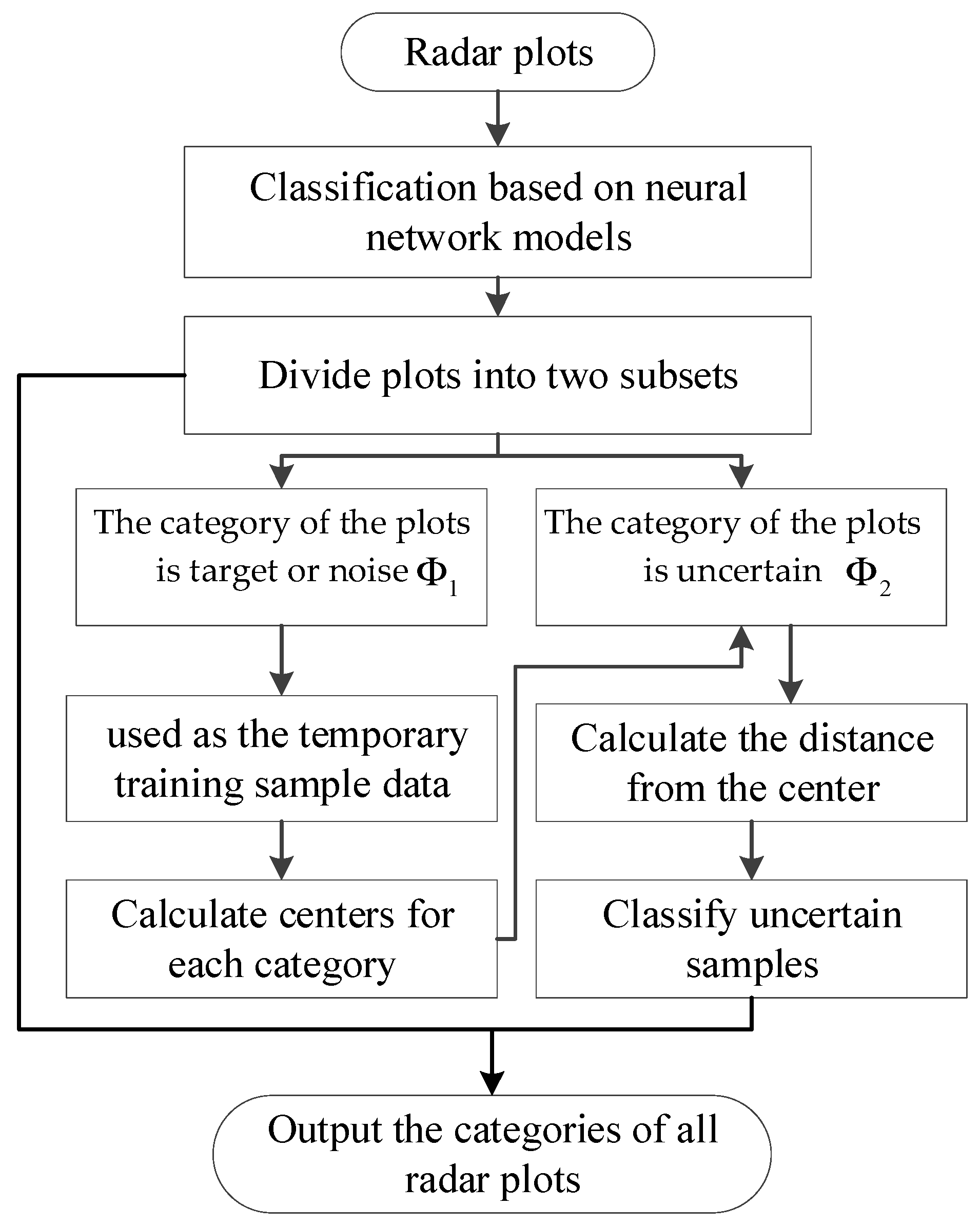
Based on the network classification model of each round, the category membership of the target can be obtained. If the network classification model is not trained, the category membership of the target will be randomly initially given. Then, the target category is updated through the correction fusion of the belief function, and the sample data after updating the category label can be used for classifier training and parameter optimization. The optimized classifier can also be reused to obtain the category membership of the target. This cycle continues until the category labels of each point in the target dataset are no longer updated or iterated a certain number of times. The value of iteration times is usually related to the timeliness of engineering applications and can be reasonably configured according to specific scenarios. The specific implementation of the update strategy is as follows:

Step 1: The global mass function $m_t$ of each test sample $O_i$ can be obtained through confidence evidence fusion based on the current deep network model classifier. The target dataset can be divided into two subsets, ${\Phi }_1$ and ${\Phi }_2$, based on $m_t$, where the subsets are defined as follows:

$${\Phi }_1=\{O_i:\underset{{\mathrm{C}}_q\in \{C_o,C_n,\Theta \}}{\max {\mathrm{m}}_t{(\mathrm{C}}_q)}\ne {\mathrm{m}}_t(\Theta )\}$$

(22)

$${\Phi }_2=\{O_j:\underset{{\mathrm{C}}_q\in \{C_o,C_n,\Theta \}}{\max {\mathrm{m}}_t{(\mathrm{C}}_q)}={\mathrm{m}}_t(\Theta )\}$$

(23)

Here, the category of the sample is target or noise in subset ${\Phi }_1$, while the category of the sample is uncertain in subset ${\Phi }_2$.

Step 2: In each round of iterative updates, the samples in subset ${\Phi }_1$ can be temporarily used as training sample data $\{(O_i,Y_i),i=1,\cdots ,N_{{\Phi }_1}\}$ after being classified by the deep learning network model. $N_{{\Phi }_1}$ is the total number of samples in dataset ${\Phi }_1$, and $Y_i$ is the category label of target $O_i$. Then, by combining the mass function of each sample, the center of this pattern category can be obtained as follows.

$$m_{{\mathrm{C}}_q}={\displaystyle \sum _{{\mathrm{C}}_q\subseteq \{C_o,C_n\},O_i\in {\Phi }_1}{m}_t(O_i)}/N_{{\Phi }_1}$$

(24)

Step 3: For the sample $O_j$ in subset ${\Phi }_2$, the confidence similarity $d$ between it and the center of categories $C_o$ and $C_n$ is calculated separately.

$$d(O_j,{\mathrm{C}}_q)=‖m_t(O_j)-m_{{\mathrm{C}}_q}‖{,}_{} {\mathrm{C}}_q\in \{C_o,C_n\}$$

(25)

According to the value of confidence similarity, the sample data are sequentially assigned to the pattern categories with the closest confidence.

In RPREC, the iterative update process of target category confidence is shown in Figure 4.

Based on the above implementation process, it can be seen that easily classified plots can provide additional evidence to help classify uncertain plots, especially in cases where clutter and target plots have high similarity in the feature space. This is also the advantage of the iterative optimization classification strategy.We summarize the RPREC in Algorithm 1.

Algorithm 1. RPREC Algorithm.

Require: Radar data set $O=\{o_1,\cdots ,o_n\}$; Classification threshold T1 and T2; Deep learning classifier; Number of Decision Evidence K; Maximum number of iteration updates Th; Initialization: Set the number of network layers and nodes in each layer. If there are samples with class labels, the classifier is initially trained based on recognition framework $\Omega =\{C_o,C_n,\Theta \}$. 1: s ← 0; 2: repeat 3: Calculate the category membership ${\mu }_i=({\mu }_{i1},\cdots ,{\mu }_{ic})$ of each target $O_i$; 4: Calculate the total belief of each category: $Bel(C_o)$, $Bel(C_n)$, $Bel(\Theta )$. 5: Calculate the number $K_i$ of samples that should be selected in each pattern category based on Equation (11), and build the decision evidence set ${\Phi }_K(i)$ of each target $O_i$; 6: Calculate the confidence similarity $M_{ij}$ between the target data and the decision sample; 7: Build the basic confidence assignment function $m_i$ for each sample; 8: Combine the evidence in the decision evidence subset $T_q$ with the same category, and obtain fusion confidence assignment function $m_t^{T_q}$; 9: Calculate the evidence discount factor $W_{C_q}$, and Obtain correction evidence $d{m}_t^{T_q}(C_q)$; 10: Combine the correction evidence and obtain the global mass function $m_t$; 11: Calculate the confidence level $Bel$ of target $O_i$ belonging to each pattern category; 12: Update category labels for each target data based on classification rules; 13: s ← s + 1; 14: until s = Th or the category labels of each target is no longer updated; 15: return the category assignment relationship of each target ${\{m(O_i,{\mathrm{C}}_q)\}}_{i=1}^N$

4. Experiments

In this section, some experimental results using real radar plots are presented, showing the effectiveness of the RPREC. All algorithms were tested on the MATLAB platform. The software used in these experiments is MATLAB R2023a under a Windows 11 system. We give an evaluation of the recognition accuracy and the run time of the considered radar plot recognition algorithms. The computations were executed on a Microsoft Surface Book with an Intel (R) Core (TM) i9-12900HX CPU @2.5 GHz and 16 GB MEMORY. There are mainly two types of scenarios: one is high-density clutter, and the other is low-density clutter. The datasets used are all collected from the X-type ATC radar. Each group of plot data is processed by a track processing program. According to the test environment and plots, the possible false track and the real track are both retained. Firstly, mark the plot data corresponding to the real track as the target. Then, mark the plot data corresponding to the false track as uncertain. Finally, mark the rest of the plots as clutter.

• The dataset with high clutter density

As shown in

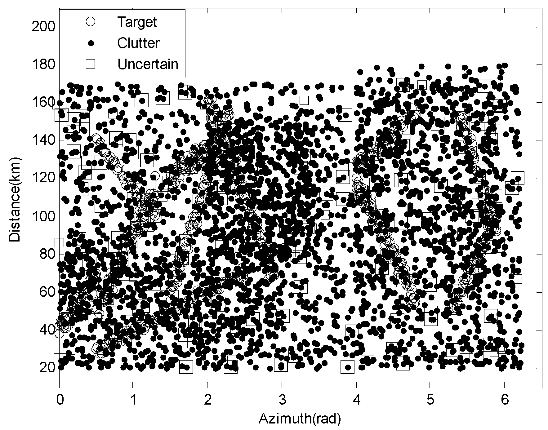
Table 1. The sample dataset with high-clutter density.

Dataset 1	Target	Clutter	Uncertain
Number	1150	2350	325

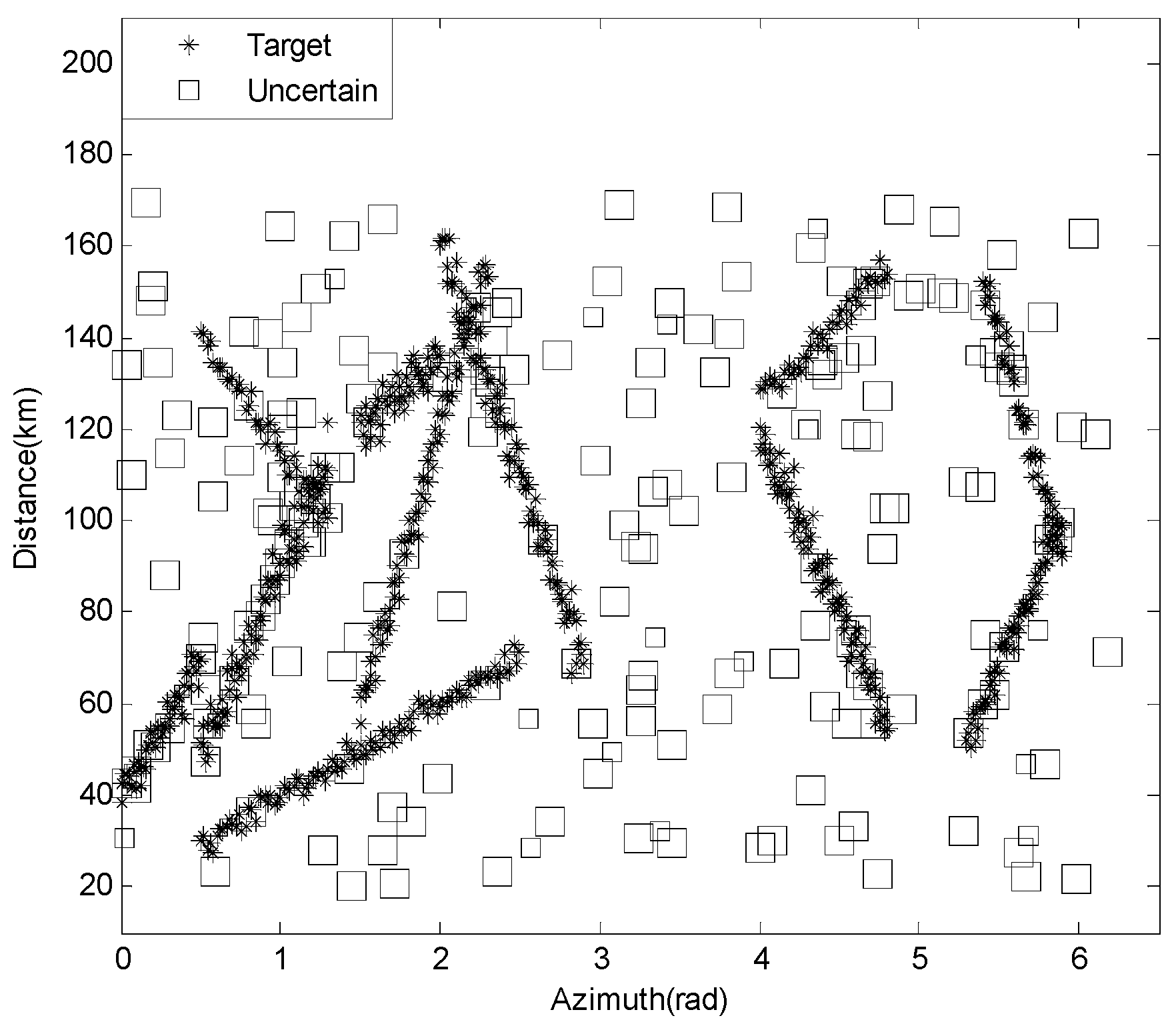
, the dataset with high-clutter density includes 1150 targets, 2350 clutters, and 325 uncertainties, and their specific distribution is shown in Figure 5. The distribution of data containing only targets and clutter is shown in Figure 6.

In Figure 6, it can be seen that the target plots are very clear and easy to identify when not affected by clutter. In Figure 5, some target plots are almost completely submerged by clutter, which poses a certain challenge to the performance of recognition algorithms.

2.

The dataset with low-clutter density

As shown in

Table 2. The sample dataset with low-clutter density.

Dataset 2	Target	Clutter	Uncertain
Number	171	213	19

, the dataset with high-clutter density includes 171 targets, 213 clutters, and 19 uncertainties, with a specific distribution as shown in Figure 7.

As shown in Figure 7, under low-clutter density, the target plot is clearly visible, while uncertain data are mainly distributed near the intersection of different target plots. This dataset is mainly used to verify the performance of each algorithm when the sample size is small.

Specific experimental verification is carried out from four aspects. First, the performance of the RPREC is evaluated with respect to some classical radar plot recognition algorithms in Section 4.1. In Section 4.2, the correlation between recognition accuracy and iteration number is provided. In Section 4.3 and Section 4.4, the impact of algorithm parameters, such as classifier iteration updates and confidence threshold on algorithm performance, is analyzed.

4.1. Radar Plot Recognition

This experiment is based on two types of radar-measured datasets, high-density clutter, and low-density clutter, which have been introduced at the beginning of Section 4. In each scenario, half of the radar plot data were randomly selected as training samples, and the remaining were used as testing samples. In order to effectively verify the performance of the RPREC, we compared it with some classic radar dot recognition algorithms, including PSO-SVM [3], PSO-MLP [54], FNN [53], CNN [55], and RNN [56]. Here, the percentage of recognition accuracy and CPU time are used as important indicators to measure the performance of these algorithms.

The experimental results based on the high-density clutter dataset are shown in

Table 3. The recognition accuracy and CPU time of six different algorithms on the high-density clutter dataset.

The Radar Plots	Recognition Accuracy/CPU Time (s)
	PSO-SVM	PSO-MLP	FNN	CNN	RNN	RPREC
ω1	0.821/0.52	0.853/0.73	0.861/1.21	0.911/2.71	0.923/3.55	0.921/9.55
ω2	0.837/1.12	0.847/1.71	0.832/3.26	0.913/5.13	0.927/6.32	0.932/18.35
ω3	/	/	/	/	/	0.945/3.37
All	0.829/1.64	0.850/2.44	0.847/4.47	0.902/7.84	0.925/9.87	0.932/31.27

, and the experimental results based on the low-density clutter dataset are shown in

Table 4. The recognition accuracy and CPU time of six different algorithms on the low-density clutter dataset.

The Radar Plots	Recognition Accuracy/CPU Time (s)
	PSO-SVM	PSO-MLP	FNN	CNN	RNN	RPREC
ω1	0.852/0.12	0.833/0.43	0.821/0.89	0.851/1.08	0.873/1.32	0.923/12.55
ω2	0.856/0.31	0.842/0.98	0.812/1.09	0.863/1.53	0.857/2.21	0.936/15.39
ω3	/	/	/	/	/	0.925/11.37
All	0.854/0.43	0.836/1.41	0.817/1.98	0.857/2.61	0.865/3.53	0.928/39.31

. In these tables, ω₁, ω₂, and ω₃ represent, respectively, target, clutter, and uncertainty.

The experimental results shown in Table 3 indicate that PSO-SVM, PSO-MLP, FNN, CNN, and RNN have some shortcomings in the representation of uncertain data. Therefore, these algorithms focus on the binary classification of targets and clutter, so the uncertain data represented by ω₃ will be hard to classify into targets or clutter. This will affect their recognition accuracy. The recognition accuracy of PSO-SVM is about 0.83, and the CPU time is 1.64. The recognition accuracy of PSO-MLP and the FNN is similar, but the FNN takes more time. Compared to the FNN, the RNN and CNN have advantages in deep feature extraction of radar plots, resulting in a higher recognition accuracy of over 0.91. Of course, the CPU time has also doubled accordingly. The most significant feature of the RPREC proposed in this article is its ability to characterize and measure uncertain data. Therefore, it can be seen from the fifth row in Table 3 that uncertain plots have been effectively identified with a recognition accuracy of 0.945. In addition, the RPREC also maintains good performance in target and clutter recognition, with recognition accuracy rates of 0.921 and 0.932, respectively. However, the RPREC also has a significant limitation in that it has a large CPU time, which is 3 to 15 times that of other algorithms.

The experimental results shown in Table 4 indicate that in low-clutter datasets with fewer radar plots, the recognition accuracy of all algorithms decreases, except for PSO-SVM and the RPREC. The reason is that PSO-SVM is an optimization algorithm of SVM, which is very suitable for small samples and can achieve a recognition accuracy of 0.854. In this case, its recognition performance is similar to the RNN. Comparing Table 3 and Table 4, it can be found that the recognition accuracy of PSO-MLP, FNN, CNN, and RNN has decreased by approximately 2 to 6 percentage points. The reason why the RPREC is not also significantly affected is that its classifier can iteratively learn the inherent characteristics of radar plots and maintain optimization, but the cost is that the CPU time is several times that of other algorithms.

Overall, PSO-MLP, FNN, CNN, and RNN perform well in high-clutter density radar point datasets, while PSO-SVM can demonstrate its advantages in low-clutter density radar point datasets. The RPREC maintains good performance in both datasets but has the highest CPU time. Therefore, in terms of being able to adapt to various different scenarios, the RPREC is the best. But if we pursue computational timeliness, the RPREC is not the best choice.

4.2. The Impact of Training Sample Sets

As is well-known, the performance of recognition algorithms is usually closely related to the training samples. Therefore, the impact of the training samples on each algorithm is mainly analyzed in this section. The dataset used here is a mixture of high-clutter density and low-clutter density samples. It has a total of 4228 radar plots, including 1321 target plots, 2653 clutter plots, and 344 uncertainty plots. Four different scenarios are set here, represented by S1, S2, S3, and S4. In each scenario, a certain number of samples are selected for classifier model training, and the remaining samples are used to test the performance of each algorithm. The specific number of training and testing samples for S1 to S4 is set in

Table 5. The training and sample testing settings in different experimental scenarios.

Experimental Scenario	Training Samples/Testing Samples
	Target	Clutter	Uncertain
S1	200/1121	500/2036	100/244
S2	300/1021	1000/1563	150/194
S3	500/821	1500/1063	200/144
S4	900/421	2000/563	250/94

. Here, the recognition accuracy and CPU time are also used as evaluation indicators. The test results of each algorithm are summarized in

Table 6. The recognition accuracy and CPU time of different algorithms.

Scenario	Recognition Accuracy/CPU Time (s)
	PSO-SVM	PSO-MLP	FNN	CNN	RNN	RPREC
S1	0.852/2.12	0.833/3.43	0.821/4.89	0.841/7.08	0.843/8.32	0.923/52.55
S2	0.856/1.31	0.852/2.98	0.842/4.09	0.863/5.53	0.894/6.21	0.936/35.39
S3	0.873/1.24	0.881/2.44	0.877/3.47	0.903/4.03	0.925/5.92	0.931/29.27
S4	0.871/1.03	0.906/1.41	0.895/1.98	0.927/2.61	0.931/4.53	0.929/18.31

.

Table 6 shows that PSO-MLP, FNN, CNN, and RNN are significantly affected by the number of samples. For example, in the S4 scenario with sufficient samples, the recognition rate of each algorithm can be about 6 to 9 percent higher than S1 with insufficient samples. At the same time, the CPU time of these algorithms is also reduced, as the number of test samples is also decreasing. The recognition accuracy of PSO-SVM does not significantly improve with an increase in the number of training samples from S1 to S4, which are generally only around 0.1 to 0.2. It can be seen that PSO-SVM is a good choice in small sample datasets. The recognition accuracy of the RPREC is also not significantly affected by the number of samples but at the cost of sacrificing a significant amount of time to optimize the classifier. So, it can be seen that the time for S4 is 19.31, but S1 requires 42.55, which is almost three times higher.

In addition, compared to other algorithms, the proposed algorithm can basically maintain the best recognition accuracy. Of course, it inevitably has the most CPU time in each scenario. This is because the classifier in other algorithms only needs to be trained offline and can be directly applied during testing. However, the RPREC needs to continuously analyze radar plots during the testing process to optimize the classifier. Specifically, the network model classifier of the proposed algorithm needs to be trained by certain samples in advance. Then, the self-learning of the classifier can be achieved through iterative updates of the class confidence of the target data, ultimately gradually improving the classification accuracy. This is why the fewer training samples, the longer it takes for the classifier to optimize to good performance. Therefore, how to maintain good timeliness like other algorithms is also the focus of future research.

4.3. The Impact of Iteration Times

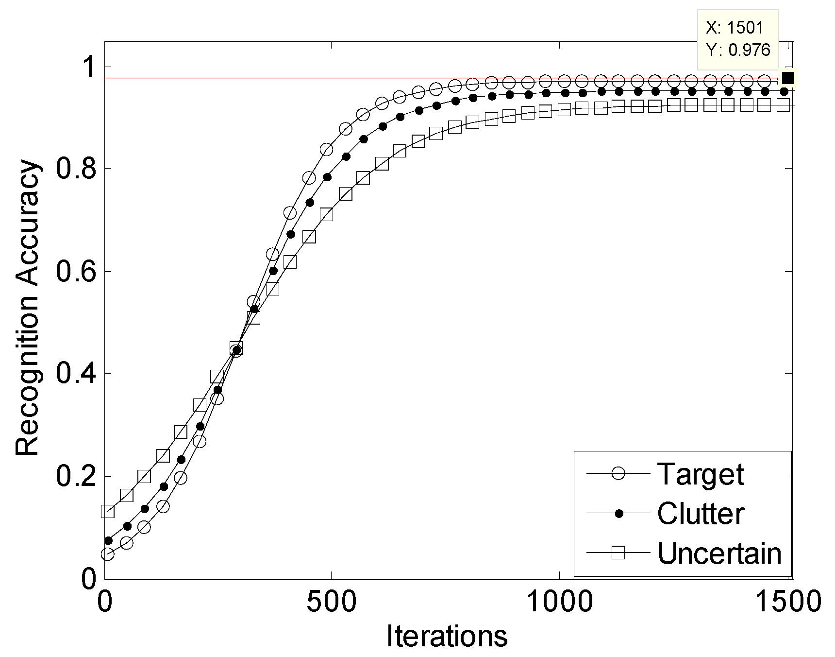
In this section, the relationship between the recognition accuracy, CPU time, and classifier iteration times of the RPREC is mainly analyzed. The specific relationship curve between the recognition accuracy and the number of iterations of the classifier in the RPREC is depicted in Figure 8. We conducted three repetitive experiments based on the same dataset described in Section 4.2. Then, the classifier was updated with 200, 500, 1000, and 1500 iterations in each experiment. Finally, the statistical results of each experiment, including recognition accuracy and CPU time, are recorded in

Table 7. The statistical results under different iterations for each experiment.

Experiment Number	Iterations	CPU Time (s)	Recognition Accuracy
Exp. 1	200	4.35	0.339
	500	10.39	0.857
	1000	25.83	0.951
	1500	35.21	0.952
Exp. 2	200	3.13	0.323
	500	12.27	0.876
	1000	23.69	0.935
	1500	35.78	0.934
Exp. 3	200	3.31	0.359
	500	9.36	0.867
	1000	22.57	0.961
	1500	37.31	0.962

.

It can be seen that once the recognition accuracy of the RPREC reaches a certain level, it will not significantly improve with an increase in iteration times. As shown in Figure 8, the recognition accuracy of targets, clutter, and uncertainty is always difficult to reach 0.98. When the number of iterations exceeds 1000, it will approach its upper limit of 0.976.

Table 7 shows that the CPU time is basically proportional to the number of iterations in each experiment. When the number of iterations reaches 500 from 200, the recognition accuracy can be quickly improved, from around 0.35 to over 0.93. When the number of iterations increased from 500 to 1000, the improvement in recognition accuracy slowed down by about 10 percentage points. When the number of iterations exceeds 1000, there is no significant change in recognition accuracy as the number of iterations increases. For example, in these three experiments, they remained around 0.951, 0.935, and 0.961, respectively. This indicates that the classifier initially improves its ability with the learning of radar plots and then reaches a certain level of performance that cannot be further improved with iterative learning, which can only increase CPU time. Therefore, the reasonable setting of parameters requires a comprehensive requirement for recognition accuracy and timeliness based on specific scenarios. Of course, it is necessary for us to further carry out research on adaptive parameter configurations that can adapt to different radar plots in the future.

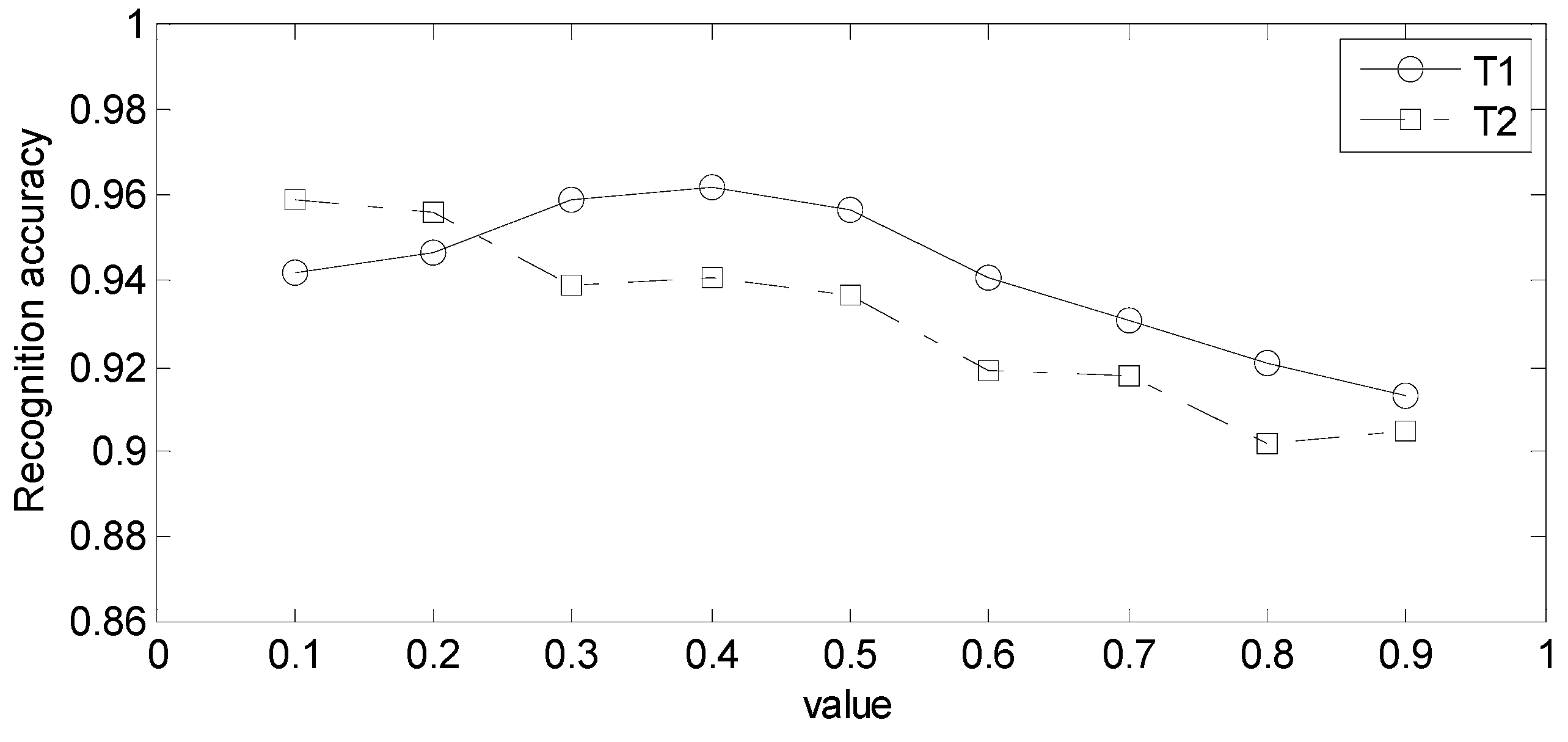
4.4. Confidence Threshold Parameter

In this section, the impact of thresholds T1 and T2 on the recognition performance of the proposed algorithm is analyzed. Here, three performance evaluation indicators, including recognition accuracy, CPU time, and number of loop iterations, were selected in this experiment. For simplicity, the Ra, Ct, and Li in the table are, respectively, used to represent recognition accuracy, convergence time, and iteration number. The statistical values of these three indicators are based on the average results obtained from 1000 Monte Carlo simulations. The experimental results are shown in

Table 8. The recognition results under different values of T1.

T1	Ra	Ct (s)	Li
0.1	0.942	8.73	1297
0.2	0.947	8.91	1284
0.3	0.959	9.15	1389
0.4	0.962	9.36	1458
0.5	0.938	8.62	1245
0.6	0.941	9.02	1231
0.7	0.931	9.51	1321
0.8	0.921	9.32	1297
0.9	0.913	8.79	1193

and

Table 9. The recognition results under different values of T2.

T2	Ra	Ct (s)	Li
0.1	0.959	16.92	2831
0.2	0.956	15.30	2627
0.3	0.935	14.97	2398
0.4	0.941	14.92	2291
0.5	0.937	9.36	1530
0.6	0.919	9.16	1439
0.7	0.922	9.28	1481
0.8	0.918	8.75	1321
0.9	0.912	8.12	1021

and Figure 9.

As shown in Table 8, when the value of T1 is changed, both Ct and Li do not show significant changes. As shown in Figure 9 the recognition accuracy of the algorithm increases first and then decreases as the T1 value increases. When the value of T1 is 0.4, the algorithm’s recognition accuracy can reach the maximum value of 0.962 calculated in this experiment. The reason is that when the T1 value is small, the algorithm’s ability to eliminate clutter will decrease, leading to an increase in the number of false targets. The high value of T1 can improve the suppression of clutter plots, but it also reduces the algorithm’s ability to recognize real targets, which are similar to clutter. Therefore, according to experimental statistical analysis, a T1 value of 0.4 is the best in this scenario.

The experimental results in Figure 9 show that as the value of T2 increases, the recognition accuracy of the proposed algorithm gradually decreases. This indicates that minimizing the uncertainty interval of the target’s category is more helpful in accurately distinguishing true from false, but it will inevitably affect the convergence speed of the proposed algorithm. Therefore, the experimental results in Table 9 show that as T2 decreases, the values of Ct and Li both increase. So, if there is enough time, a value of 0.1 for T2 is the best choice for this scenario.

Therefore, the reasonable setting of thresholds T1 and T2 parameters is a challenge in the RPREC. What we need to pay special attention to is the effective adjustment of parameters, which will depend on the specific situation in the future.

5. Conclusions

In this paper, the RPREC was proposed to improve the recognition performance of radar plots with the help of a deep neural network classifier where the basic confidence assignment of an object can iterate loop optimization. The RPREC first constructs a confidence framework for targets, clutter, and uncertainty categories to effectively represent radar plots. Then, a deep network model classifier is used to obtain the class confidence of each object online, and decision evidence is used to correct and update class labels. Finally, the updated data drive the classifier to complete iterative optimization, thus achieving accurate recognition of radar plots. The effectiveness of the proposed algorithm based on the real radar plot dataset has been verified. The experimental results show that the recognition accuracy of the RPREC can reach almost 93%, which is superior to traditional recognition algorithms. In addition, the RPREC can also gradually improve recognition ability by iteratively learning the inherent distribution characteristics of sample data when the number of samples is small.

In the future, this research topic can be further explored by integrating the RPREC with adaptive parameter configuration. This enables the recognition algorithm to be better applied to various types of radar plot scenarios.