1. Introduction
With the development of fifth-generation (5G) technology and the emergence of diverse services, a wide variety of quality of service (QoS) demands are placed on existing communication networks [
1]. In order to meet the different needs of terminal devices using existing communication networks, network slicing (NS) technology has emerged. NS technology divides the traditional physical network into multiple dedicated, virtualized, customized, and isolated logical networks, where each slice is used to fulfill the requirement of a specific service [
2]. The current diverse scenarios for NS services are mainly categorized into enhanced mobile broadband (eMBB), ultra-reliable, low-latency communication (URLLC) and massive machine-type communication (mMTC) services [
3]. Different scenarios have different requirements for network resources, which determines the differentiated services they can provided. The eMBB services are mainly suitable for high data rate application scenarios, such as ultra-high-definition video transmission, virtual reality, live streaming of races, etc. The URLLC services are mainly targeted at low-latency and high-reliability application scenarios, such as autonomous driving, 5G smart factories, remote surgery, etc. The mMTC service are mainly suitable for scenarios with a high number of terminal connections, such as smart home, automatic meter reading, smart agriculture, etc.
NS uses network function virtualization (NFV) and software-defined networking (SDN) technology to manage and allocate resources to achieve logical unified management and flexible control. As a result, the use of the above technology has resulted in a significant increase in resource utilization [
4]. More specifically, NFV abstracts general servers as computing resources, storage resources, and network resources in the network, manages them uniformly, and then divides them on demand. Using NFV technology, previously dedicated communication network equipment can be replaced with general high-performance servers, and communication network functions are implemented via virtual network functions (VNFs) running on virtual machines (VMs) [
5]. SDN enables the separation of the control plane and the data plane, making the network much more flexible and scalable.
NS has many features such as end-to-end (E2E), isolation, flexibility, customization, and so on. First, the E2E concept indicates that the slice is an E2E network with the ability to provide network services independently. Therefore, the resource allocation of the radio access network (RAN) and the core network (CN) should be considered together. Isolation means that any changes in one slice (e.g., addition of users, changes in channel state information, etc.) will not affect the operation of other slices. Flexibility is reflected in the fact that the network elements that make up the slices can be deployed independently or shared for scheduling. Customization indicates that slicing provides on-demand logical network topology and connectivity for different industries, services, or users to meet their differentiated QoS.
3GPP states that networks can be classified into two main categories: Public Land Mobile Network (PLMN) and non-public network (NPN) [
6]. PLMN is a communication network built by mobile network operators (MNOs) for public users, which is most closely related to our daily life. NPN achieves network signal coverage in specific areas. It provides communication services within the enterprise according to the characteristics of the industry. It can be understood as a supplement to the public network. NPN requires high reliability as well as high security. High reliability is reflected in the priority to ensure that the QoS of NPN is not affected when the resources are relatively insufficient. High security is demonstrated by the fact that the resources used by NPN are relatively independent, which ensures that private data within the enterprise is not exposed. NPN can be deployed in two ways [
7]: (i) Standalone NPN (S-NPN), where enterprises use a dedicated band and deploy a full 5G network independently. Since it is completely isolated from the PLMN, it can effectively protect the enterprise’s data security. The disadvantage is that it is very costly and not suitable for most enterprises. (ii) Public network integrated NPN (PNI-NPN), where the NPN shares some infrastructure with the PLMN to accomplish the network’s deployment. NPNs are usually implemented by creating dedicated network slices [
8]. Hence, the main issue considered in this paper is the resource allocation in the scenario of the integration of PLMN and NPN, which are both achieved via NS.
The resource allocation problem of the NS mainly includes two parts: the resource allocation of RAN and the VNF mapping of CN. For the resource allocation of RAN, ref. [
9] focuses on efficient sharing of radio resources among different users while guaranteeing the service requirements. Although this approach usually results in higher multiplexing gains, it does not guarantee performance isolation. A two-level RAN RB resource allocation method is proposed in [
10]. It is assumed that when the pre-allocated RB resources of a base station are insufficient, it is allowed to borrow additional RB directly from other base stations. It has the advantage of reducing the signaling overhead and providing an immediate service response to end users. But, the isolation between slices is also not considered. Ref. [
11] proposed a resource scheduling scheme that consists of deep learning (DL) in conjunction with reinforcement learning (RL). The main goal is to satisfy the users’ QoS requirements with as few resources as possible while satisfying the isolation requirement. The advantage is that DL and RL are integrated together and the isolation of slices is taken into account. The disadvantage is that it only considers the allocation of resources to slices, but it does not continue to allocate them to end users. In [
12], a two-layer resource allocation framework is proposed, where the upper and lower layers correspond to the Centralized Unit or Distributed Unit (CU/DU) side and the Remote Radio Unit (RRU) side, respectively. After that, a Q-learning-based NS resource allocation scheme is proposed to maximize the total utility of the whole network. Ref. [
13] mainly addresses the problem of bandwidth allocation for deep reinforcement learning-based NS. It enables the weighted sum of spectral efficiency and quality of experience (QoE) to be maximized. For the VNF mapping of CN, ref. [
14] proposed a scheme based on the feature decomposition method to implement VNF mapping and traffic control. However, only simple graph mapping relationships are considered, which do not involve the processing of dynamic services and cannot meet the real-time requirements of services. Ref. [
15] presents the VNF placement problem in NS, where the optimization problem is to minimize the reliability degradation and cost while maintaining strict delay constraints. A Tabu search-based algorithm is used to find a solution. In [
16], a VNF deployment scheme that maximizes operational benefits is proposed to ensure the reliability of the network. Ref. [
17] proposed a graph neural network-based algorithm to predict the resource demand by using the topological information of the VNF forwarding graph, thus reducing the failure rate of slices.
However, the research above on the resource allocation for NS does not address NPN slices. In other words, only the QoS requirements of different slices are considered, and the differences between public and non-public network slices are not taken into account. Therefore, in this paper, we focus on the resource allocation problem in the scenario where public network slices (including eMBB slices and URLLC slices) and non-public network slices (NPN slices) coexist. Compared with public network slices, the characteristics of NPN slices are reflected in two aspects: (i) NPN slices require higher service priority and reliability; and (ii) NPN slices require higher security and privacy. In addition, we summarize the related works and compare them with our work in
Table 1.
In this paper, we first formulate the E2E resource allocation problem with both public and non-public slices, which is a nonlinear integer programming problem. Next, due to the nature of the problem, we split the joint optimization problem into two sub-problems: the RB allocation problem and the feasibility problem of VNF mapping. Then, a combination of deep reinforcement learning (DRL) and machine learning (ML) algorithms are used to solve the problem. More specifically, DRL is employed to provide the RB allocation scheme that makes the objective function, which is the network operator’s profit, as large as possible. ML assists in determining whether the allocation scheme provided by DRL satisfies the constraints, thus helping the DRL agents to receive fast reward feedback. For deep reinforcement learning, we use multi-agent reinforcement learning to reduce the action space, and the specific algorithm employed is independent proximal policy optimization (IPPO). For machine learning, we speed up the solution feasibility determination by training a binary classifier, and the specific algorithm used is random forest (RF). Therefore, we name the proposed algorithm the IPPO-RF algorithm. The simulation results show that the IPPO-RF algorithm has good performance, i.e., not only are all the constraints satisfied, but the service priority and security of the NPN slices are ensured. The main contributions of this paper can be summarized as follows.
We solved the resource allocation problem associated with E2E network slicing, which involves both the RB allocation problem in the RAN and the VNF mapping problem in the CN.
We focus on the resource allocation problem in the scenario where public network slices (including eMBB slices and URLLC slices) and non-public network slices (NPN slices) coexist. Compared with public network slices, the characteristics of NPN slices require higher reliability and higher privacy.
We innovatively utilize a collaborative approach, combining DRL and ML, to address the E2E resource allocation problem of network slicing. The significance of the algorithm above lies in its contribution of a valuable approach for solving similar problems.
The rest of the paper is organized as follows. The system model is presented in
Section 2. In
Section 3, we first describe how to split the joint optimization problem of this paper into two sub-problems. Next, a combination of DRL and ML algorithms are introduced to solve the problem. In
Section 4, we present the simulation results as well as discussions, and finally, we conclude the paper in
Section 5.
2. System Model
In this paper, we consider an end-to-end (E2E) NS system where public and non-public network slices coexist. In terms of public network slicing, since most of the researchers primarily focus on eMBB and URLLC slices, we take them into account. Thus, a total of three types of slices are considered: eMBB slices, URLLC slices, and NPN slices. The system architecture is shown in
Figure 1.
The system consists of two parts: the radio access network (RAN) and the core network (CN). These two parts are connected via the backhaul links. The RAN is mainly responsible for allocating wireless spectrum resource blocks (RBs) to users in the slice. The CN mainly maps the VNFs to general servers in the physical network.
2.1. Radio Access Network Domain
We assume a specific area composed of a set of gNodeBs
. The three types of slices considered, namely the eMBB slices, the URLLC slices, and NPN slices, are denoted by
, and
, respectively. The set of slices is represented as
. Randomly located in the area are the end-users
, which are eMBB users, URLLC users, and NPN users, i.e., each user belongs to one and only one slice. The set of users belonging to Slice
s can be represented as
,
. We assume that each end-user
is served by the nearest gNodeB, denoted as
. Considering the limited coverage of the NPN, we assumes that the NPN slice is served by only one gNodeB. We consider a downlink (DL) transmission scenario based on orthogonal frequency division multiple access (OFDMA). The spectrum resources can be represented as a shared RB pool
, where the RB are organized as a resource grid and each RB is the minimum scheduling unit [
18]. we define a binary variable
as an indicator for assigning RB
k to user
u in slice
s:
We assume that each RB can be assigned to at most one user, thus reducing interference and ensuring the isolation of slices. This constraint can be expressed as follows:
We further assume that the gNodeBs have a near perfect knowledge of the channel state information (CSI). The achievable data rate of the user
u belonging to slice
s is defined as follows:
where
W represents the bandwidth of an RB;
is the downlink transmission power; and
is the channel gain between the gNodeB
and the end-user
, including Pathloss and Rayleigh fading [
19].
is the power of the additive white Gaussian noise (AWGN). We assume that the downlink transmission power is the same for all RBs. We assume that the set of gNodeBs we consider is a gNodeB sharing group, more specifically, all the gNodeBs share a common RB pool [
20]. Therefore, there is no frequency reuse in the same gNodeB sharing group. Furthermore, we have made the assumption that each RB can be assigned to at most one user. Thus we do not consider interference in Equation (
3).
Therefore, the total rate of slice
s can be expressed as:
To calculate the RAN delay of user
u in slice
s, we follow [
10,
21,
22], where the queue traffic model is formulated as an M/M/1 queuing model. We make the following assumptions: (i) the arrival process of each user packets follows a Poisson distribution, and (ii) the inter-arrival times of the packets are independent and follow an exponential distribution with mean
. Thus, the packets arriving and serving process in slice
s can be modeled as
independent M/M/1 queuing systems. By applying Little’s law, the RAN delay of the user
u in slice
s is:
where
and
denote the packet size and the packet arrival rate of user
u in slice
s, respectively. The first and second terms in the denominator represent the processing and arrival rates of user packets, respectively. We assume that users within the slice have the same packet size and packet arrival rate. The packet size for each slice is denoted by
, respectively. The packet arrival rate for each slice is denoted by
, respectively.
2.2. Core Network Domain
We consider the physical network as a directed graph , where represents the set of server nodes, and represents the set of links between server nodes. The resources of each server usually include CPU, memory, disk, etc. In this paper, in order to simplify the model, various resources on nodes are unified as computing resources. The available computing resources of all server nodes are denoted as . The number of virtual machines (VMs) that the server nodes host is represented as . The set of link bandwidths between the server nodes is represented as , and the set of link delays between server nodes is represented as . Note that if there is no directed edge from Server node a to Server node b, then the link bandwidth and the link delay . The link bandwidth from a node to itself is specified to be infinity, i.e., , while the link delay is zero, i.e., .
VNF is a type of network function implemented in the software and it operates on physical servers. Different VNFs can be arranged in a specific sequence to create a service function chain (SFC), enabling the provision of complex network services. The VNFs we are considering primarily include a firewall (FW), network address translator (NAT), traffic monitor (TM), video optimization controller (VOC), an intrusion detection and prevention system (IDPS), and so on [
19]. Different VNFs types are needed, which is represented as
. For each slice, its SFC consists of several VNFs in a certain order. Thus, the SFC of slice
is denoted by
, where
,
, and
is the length of the SFC of Slice
s. Each VM on any server node can host at most one VNF, and multiple VNFs in the same SFC can be deployed in the same server node. The processing delay of each VNF is determined by its type. To simplify the model, we assume that the delay of each VNF type is known in advance and it can be represented as
.
When the data flow passes through the SFC of a slice, after the processing of each VNF, the data processing rate in the SFC will change. In order to easily depict the variation in the data flow in the SFC, we assume that the data processing rate through different VNFs follow linear changes, and this change is quantified by using the data rate expansion ratio [
12]. Note that the data rate expansion ratio depends on the type of the VNF; hence, we collect the data rate expansion ratio of all VNF types and denote it by
. Thus, the data processing rate through the
j-th VNF in the SFC of Slice
s can be denoted by [
12]:
where
is the input data processing rate of the
j-th VNF and correspondingly,
is the output data processing rate of the
j-th VNF, which is also the input data processing rate of the
-th VNF. Note that the data processing rate of the first VNF in the SFC of Slice
s is the total rate of slice,
, where
is given in (
4).
Figure 2 illustrates an example of the data processing rate in the SFC of Slice
s:
A binary variable
is defined as an indicator to show the mapping of the VNFs in the SFC to server nodes:
The following constraint ensures that each VNF must be successfully deployed and be deployed in only one server node.
To simplify the complexity of the model, we assume the computing resources required by the VNFs to be linear with the data rate passing through the VNFs [
12]. Therefore, the relationship between the VNF computing resources required and the data processing rate is expressed as follows:
where
represents the correlation coefficient between the computing resources and the data rate.
The CN propagation delay of Slice
s is defined as the sum of the delays of each link and it can be expressed as
The CN processing delay for Slice
s is defined as the sum of the processing delays of each VNF as follows:
Hence, the total CN delay of User
u in Slice
s is given as
which is only a function of
s and not
u, i.e., for users belonging to the same slice, the CN delay is the same.
Thus, the total delay of user
u in Slice
s is
where
is given by (
5).
In order to reflect the higher security and privacy of NPN slices compared to public network slices, we require VNFs of the NPN slices to have dedicated server nodes and links. More specifically, to ensure the security and privacy of the NPN slices, we require that if a server node
v is occupied by a VNF of an NPN slice
, then VNFs of other slices cannot be deployed on this server node, i.e.,
Also, for security reasons, if a link is used by an NPN slice
, then other slices cannot use this link, i.e.,
2.3. Performance Metrics
In order to evaluate the performance of the resource allocation, we introduce the performance metrics of user satisfaction and the network operator’s profit.
In order to reflect the difference of users’ demand in the slice, we propose the personalized requirements of users (PRU). For the eMBB slices, users have individual rate requirements; for the URLLC slices, users have individual delay requirements; and for the NPN slices, users have both individual rate and delay requirements. It is important to note that the user’s personalized requirements simply reflect the rate or delay that the user anticipates, which may not be strictly guaranteed during the resource allocation. The set of PRU for these three types of slices are denoted by is an eMBB user}, is an URLLC user}, and is a NPN user}, respectively. The set of PRU can be represented as . Ideally, we would like the network to satisfy all users’ personalized requirements. However, given the limited resources, this is not always possible. In our work, we place a higher service priority on the NPN users, i.e., the resource allocation should be that the individual rate requirement and delay requirement of each NPN user is satisfied strictly. For users in other slices, personalized requirements are addressed to the best extent possible, ensuring that the overall user satisfaction remains above a certain threshold.
User satisfaction for users in the eMBB, URLLC, and NPN slices are respectively defined as follows:
Hence, as can be seen, for an eMBB user u, the satisfaction is 1 as long as the achieved rate is no smaller than the required rate . Otherwise, User u’s satisfaction depends on the ratio of the achieved rate and the required rate . Similarly, for a URLLC user u, the satisfaction is 1 as long as the achieved delay is no larger the required rate . Otherwise, it is the ratio of the required delay and the achieved delay . Since the NPN users have both rate and delay requirements, we define the user satisfaction as the average of the rate satisfaction and the delay satisfaction. Finally, the user satisfaction of a slice s is defined as the user satisfaction average of all users in Slice s.
Recall that we place a higher service priority on the NPN users, i.e., their PRU need to be satisfied strictly. In other words, we require that for users of NPN slices, which further means that the user satisfaction of any NPN slice is equal to 1.
The network operator’s profit is
where
and
represent the revenue and expenditure, respectively. More specifically, the revenue comes from the service data rate provided to the users and the expenditure mainly comes from the number of RBs used and the amount of computing resources used, i.e.,
where
as defined in (
4) is the total achieved rate of Slice
s;
as defined in (
9) is the computing resource used by the
j-th VNF of Slice
s;
is the total number of RBs used, with
defined in (
1);
represents the unit price of the service rate; and
and
represent the unit price of an RB and the computing resources, respectively.
2.4. E2E Optimization Problem
The optimization objective of this paper is to maximize the network operator’s profit while satisfying the constraint of total resources, the minimum rate, the maximum delay, the user satisfaction requirement of each slice, and the security and privacy of the NPN slices. More specifically, the E2E optimization problem is formulated as follows:
where the objective function is as defined in (
19). Note that the constraint in (22b) ensures that the number of RBs allocated to the users do not exceed the total number of RBs in the resource pool; constraint (22c) indicates that the number of VNFs deployed on each server node cannot exceed the number of VMs hosted by the server node; constraint (22d) specifies that the sum of the computing resources required by all VNFs deployed on a server node cannot exceed the available computing resources of the server node; constraint (22e) indicates that the sum of the data traffic on each link does not exceed the bandwidth limit of the link; constraint (22f) ensures that the data rate of each end-user in Slice
s, i.e.,
as defined in (
3), is not lower than the minimum rate threshold
; constraint (22g) ensures that the E2E delay of each end-user in Slice
s, i.e.,
as defined in (
13), cannot exceed the maximum delay threshold
; and constraint (22h) indicates that the user satisfaction of Slice
s should not be lower than the satisfaction threshold
, and, according to previous discussions, we have
when
s is an eMBB or URLLC slice and
when
s is a NPN slice.
The proposed problem of (22) is a binary nonlinear integer programming problem. The time complexity for solving this problem is
; furthermore, it can be reduced to a knapsack problem, which is NP hard. Hence, it is inefficient and infeasible to exhaust all possible allocation options to find the optimal one. However, Artifical Intelligence (AI) has powerful decision making and information extraction capabilities, especially deep reinforcement learning. Furthermore, many researchers have shown that AI-based resource allocation methods are more efficient than other methods [
19,
23]. Therefore, in this paper, we resort to machine learning and deep reinforcement learning approaches to solve the proposed problem (22).
3. Algorithm Design
The problem in (22) consists of two types of optimization variables:
, which indicates how to assign RBs to users in the slices in RAN, and
, which indicates how to map VNFs of all slices to the VMs of the server nodes in CN. Looking at the objective function of the problem in (22), we see that it is only a function of the allocation scheme of RBs in RAN and is not related to the mapping scheme of the VNFs in CN. Furthermore, (22b), (22f), and (
2) are constraints that only involve the RB allocation scheme, while (22c), (
8), (
14), and (
15) are constraints that only involve the VNF mapping scheme. The constraints (22d), (22e), (22g), and (22h) involve both the RB allocation scheme and the VNF mapping scheme due to the delay variables
and the rate variables
.
For problem (22), once the RB allocation scheme is fixed, the variables
is fixed and
in (
5) is fixed. According to (
4), fixed
provides fixed
; hence, given the RB allocation scheme, (22d) and (22e) becomes constraints involving only the VNF variables
. Next, we transform the constraints (22g) and (22h) to separate the effect of the RB allocation scheme and the VNF mapping scheme. First, denote the total CN delay of a User
u in Slice
s as
, which is a function of only
s, and not a function of
u according to (
12). Then, we discuss the transform of the constraints (22g) and (22h) for different types of lices.
- (1)
For User
u in an eMBB slice
s, due to (
16), the constraint (22h) only involves the RB allocation scheme. Next, we discuss the transform of (22g). To satisfy (22g),
must satisfy
according to (
13). Hence, based on (
12), for the eMBB slice
s, to satisfy (22g), the VNF mapping scheme must satisfy
- (2)
For the URLLC or NPN slice
s, to satisfy (22g),
again has to satisfy (
23). Now, we transform the constraint (22h). The term
. Hence, for User
u in the URLLC slices (NPN slices), we may express the user satisfaction
as a function of
, according to (
17) and (
18) for a fixed RB allocation scheme. Correspondingly, according to constraint (22h),
has to satisfy
for the URLLC slice
s, and
for the NPN slice
s. The left-hand side (LHS) of (
25) and (
26) are both decreasing functions of
. Hence, the bisection search method can be used to find the maximum
that satisfies (
25) and (
26), which is denoted as
. Hence, for the URLLC or NPN slice
s, to satisfy (22g) and (22h), the VNF mapping scheme must satisfy
Define
as
then, (
24) and (
27) can be expressed using a uniform expression
Therefore, we have successfully split the problem (22) into two sub-problems. The first one is the RB allocation problem, which is
and the second one is the feasibility problem of the VNF mapping, i.e., the checking of the last constraint of the problem (
30) for a given RB allocation scheme:
Note that among the constraints of the problem, (
31), (22c), (
8), (
14), and (
15) only depend on the variables
and are independent of the RB allocation scheme. For a given RB allocation scheme, the variables
are given and thus, constraints (22d) and (22e) are well defined. Furthermore, the variables
are given; thus, the constraint (
29) is well defined. Hence, for a given RB allocation scheme, the problem (
31) is well defined.
Based on this observation, to solve the problem of (22), in the outer loop, the multi-agent reinforcement learning IPPO algorithm is used on problem (
30) to decide how to allocate the RBs so as to maximize the objective function. For each RB allocation scheme considered by the outer loop, in the inner loop, the RF algorithm is used on problem (
31) to check the feasibility of the RB allocation scheme which determines whether the CN can successfully complete the mapping of the VNFs for all slices.
In the following two subsections, we will provide details on the VNF mapping problem, i.e., (
31), solved using the RF algorithm, and the RB allocation problem, i.e., (
30), solved using the multi-agent reinforcement learning IPPO algorithm, respectively.
3.1. The VNF Mapping Problem (31)
We first introduce the Deep First Search with the pruning (DFS + pruning) algorithm to determine whether the VNFs of all slices can be successfully deployed in CN such that the constraints of problem (
31) are satisfied. After that, in order to reduce the computational time overhead, we use supervised learning techniques to train an RF to determine whether all the VNFs can be successfully deployed in the CN.
3.1.1. DFS + Pruning Algorithm
Depth-First Search (DFS) is an algorithm for traversing a tree or graph, which mainly traverses the nodes of the tree or graph in the depth direction. When all children of node v have been traversed or do not satisfy the constraint, it goes back to the parent node of node v and continues traversing in the depth direction until all nodes have been visited.
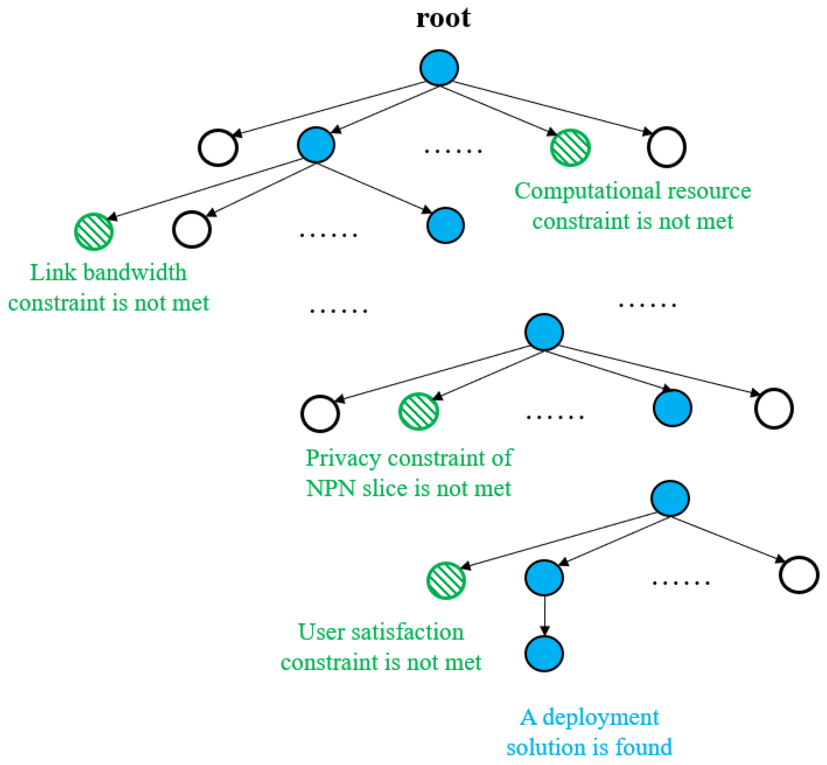
For problem (
31), the depth of the tree is the total number of VNFs, which is equal to the number of slices multiplied by the number of VNFs in each slice, i.e.,
. Recall that the number of servers is
V. The number of nodes in the first layer is
V and it represents the possibilities of the deployment of the first VNF, i.e., which server the first VNF is deployed on. For each node in the first layer, there are
V number of children node, and the second layer represents the possibilities of the deployment of the second VNF. For example, the third children node of the fifth first-layer node represents the deployment strategy, where the first VNF in deployed on Server 5 and the second VNF is deployed on Server 3. The other layers are structured accordingly, i.e., the number of children of each node is
V. An illustration of the tree is provided in
Figure 3.
The time complexity of the whole algorithm can be expressed as . In order to reduce the time complexity of the algorithm, pruning is considered to reduce the search space.
The specific pruning strategies are as follows:
The pseudo-code of the DFS-pruning algorithm is presented in Algorithm 1. During the traversal of the tree, the traversal path is recorded. It is the information about which server node the VNFs should be deployed on. Therefore, the above DFS+pruning algorithm can be used not only to determine whether the VNFs of all slices can be successfully deployed in CN, but also to find all VNF deployment schemes that meet the constraints.
| Algorithm 1 DFS + Pruning. |
Input: VNF Set of all slices ; The initial state Initial call to the function DFS(1, ) Output: Whether VNF mapping can be completed. True or False Process: Function DFS(Current Considered VNF i, current state s) - 1:
Recursive termination conditions - 2:
if
then - 3:
Indicates that all VNFs are deployed - 4:
Find a deployment scheme - 5:
return True - 6:
end if - 7:
Consider deploying current VNF i to node v in turn - 8:
for do - 9:
if node v does not satisfy the constraints of problem ( 31) then - 10:
continue - 11:
else - 12:
Record current state s - 13:
Deploy the current VNF i to node v - 14:
Update the status to - 15:
Recursive calls DFS(, ) - 16:
Restore the scene: reset the current state to s - 17:
end if - 18:
end for - 19:
return False
|
The disadvantage of the DFS+pruning algorithm is that it has a relatively high time complexity. Next, ML is considered to train a classifier to solve the problem (
31).
3.1.2. Random Forest Classifier
First, multiple sets of
are randomly generated. These would specify the constraints of the problem (
31). Then, the above DFS+pruning algorithm is used to generate the labels corresponding to the generated sets
. The labels represent whether the CN can successfully complete the VNF mapping. After that, the training set generated in the above way can be used to train a classifier to solve this binary classification problem. The classifier used in this paper is RF, which is a very powerful supervised learning algorithm.
3.2. The RB Allocation Problem (30)
We first model the problem (
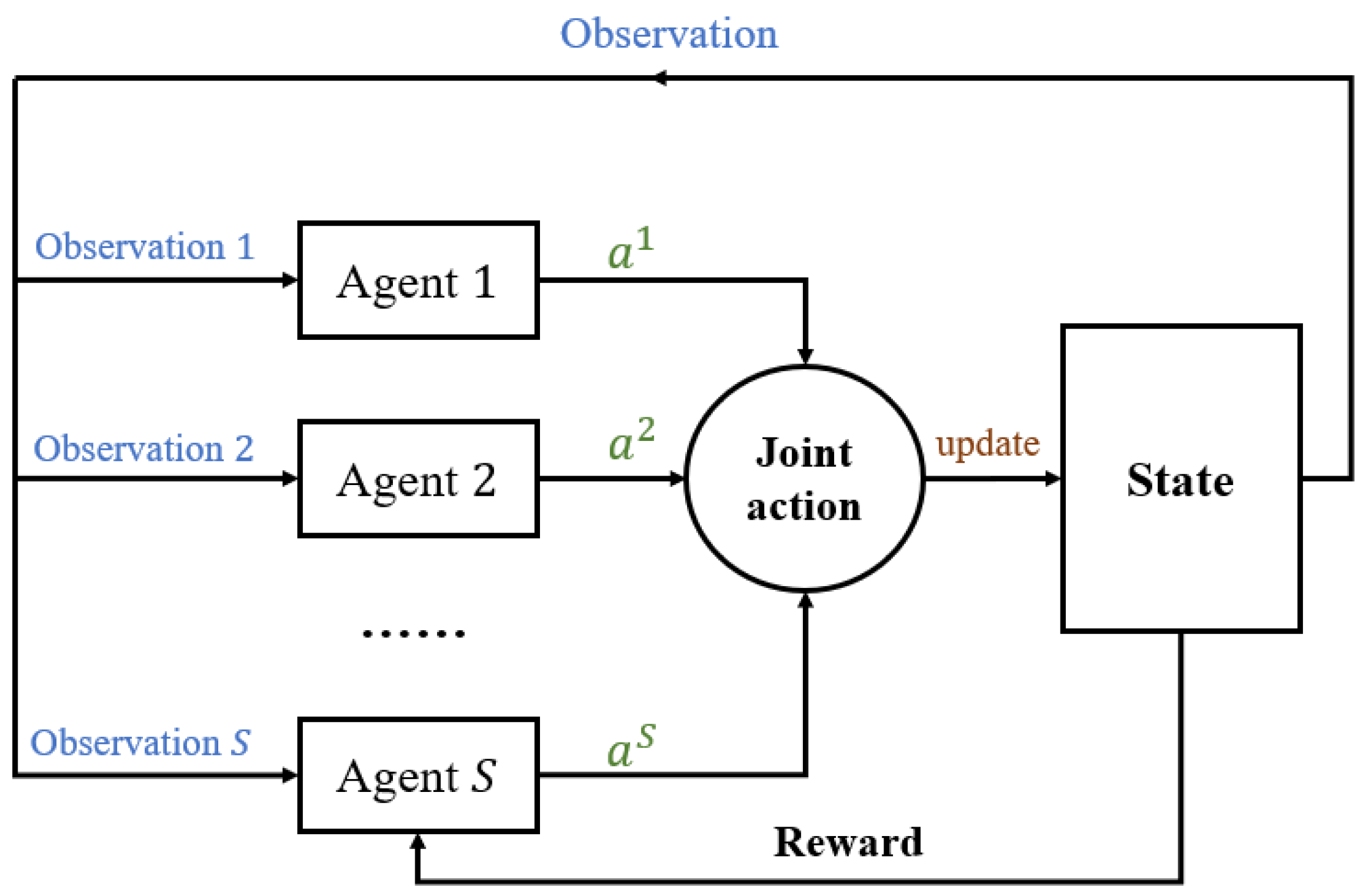
30) as a Markov Decision Process (MDP). Then, we employ the multi-agent reinforcement learning IPPO algorithm to solve the MDP.
3.3. Independent Proximal Policy Optimization (IPPO)
The MDP modeled above for this problem can be solved using various reinforcement learning methods. We tried several popular reinforcement learning methods and found that the IPPO algorithm is the most effective. Therefore, we propose to use the IPPO algorithm to solve the RB resource allocation problem of (
30).
The Proximal Policy Optimization (PPO) algorithm is an On-policy algorithm that can be used for both continuous action space tasks and discrete action space tasks. PPO is based on the idea of the Trust Region Policy Optimization (TRPO) algorithm, but its algorithm implementation is simpler and more effective.
The IPPO algorithm is the multi-agent version of the PPO. Each agent is trained independently with the PPO algorithm. PPO is based on the Actor–Critic architecture, so two neural networks, the policy network and the value network, are required in the training process. The policy network is mainly responsible for choosing actions based on the current state and policy, interacting with the environment to receive feedback, and continuously updating the policy. The value network is mainly responsible for learning the state value function, which is used to help the policy network to update the strategy. In this paper, each slice corresponds to an agent, so the number of agents is S. Therefore, the number of neural networks required for the IPPO algorithm is .
4. Simulation Results
In this paper, the simulation experiments are performed on a PC with a 12th Gen Intel(R) Core(TM) i9-12900K processor and 8 GB of RAM. To simulate the proposed problem, we use the programming language Python 3.10.4 and PyCharm Community Edition 2022.2.1. In the simulation, we consider one eMBB slice, one URLLC slice, and one NPN slice, i.e., . The users of the eMBB slice and the URLLC slice are uniformly distributed in a km area. There are three gNodeBs in this area. The users of the NPN slice are generated randomly around a particular gNodeB only. We assume that the number of users in the eMBB, URLLC, and NPN slices are 10, 10, and 5, respectively. The PRU are generated via a uniform distribution within a given interval. Specifically, the personalized rate requirement interval for eMBB users is (Mbps), the personalized delay requirement interval for the URLLC users is (ms), and the personalized rate and delay requirement interval for the NPN users is (Mbps) and (ms), respectively. We set the user satisfaction threshold of the eMBB, URLLC, and NPN slice to , , and 1, respectively, i.e., .
We assume that the SFC of the eMBB slice is VNF1 → VNF3 → VNF4 → VNF5, the SFC of the URLLC slice is VNF2 → VNF4 → VNF5 → VNF6, and the SFC of the NPN slice is VNF1 → VNF7 → VNF3 → VNF8. The core link transmission delay is uniformly distributed from 0.5 ms to 2 ms and the core link bandwidth is uniformly distributed from 10 Mbps to 50 Mbps. The remaining simulation parameters are summarized in
Table 2.
We create and train the neural networks of the IPPO using the Pytorch 1.10.2 framework. More specifically, for each agent, the Actor Network and the Critic Network both consists of two fully connected hidden layers, each with 64 neurons, and the Adam optimizer is used. With the exception that the activation function of the output layer is softmax, the activation function of the remaining layers is ReLU. The other hyperparameters of IPPO are given in
Table 3.
The RF algorithm is used to determine whether the RB allocation scheme of RAN can be successfully implemented by the VNF mapping in CN. The dataset of the RF algorithm is the randomly generated sets of
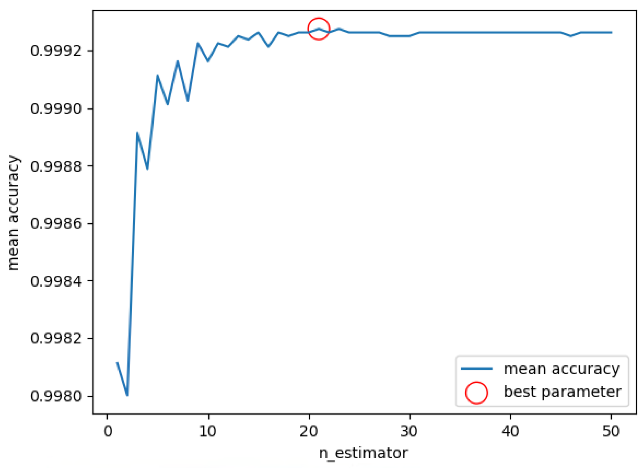
and the label is 0 or 1, which is found using the DFS+pruning algorithm. We picked 50,000 sets of data with the label 0 and 50,000 sets of data with the label 1 to train the RF. The most important hyperparameter of the RF is the number of decision trees
. To find the optimal hyperparameter, the dataset is first divided into a training set, validation set, and test set in the ratio of 3:1:1. Then, the RF is constructed with a different number of decision trees
, and the four-fold cross-validation is performed with the training set and the validation set. The mean accuracy of the cross-validation is plotted in
Figure 5 for different
values. The red circle marks the optimal point, which corresponds to
, which is the value we used to build the RF.
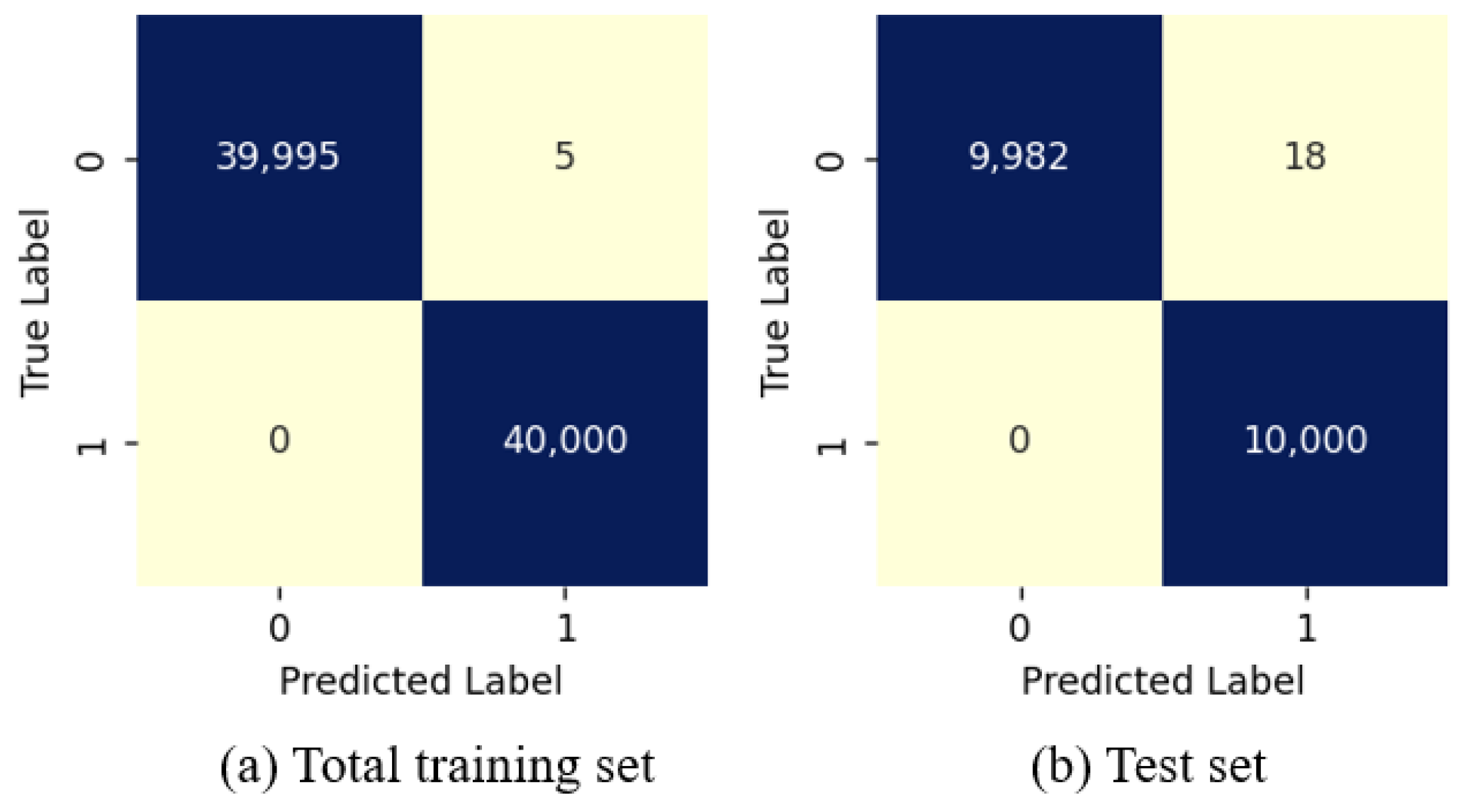
We train an RF model with the total training set, which includes the training set and the validation set. The accuracies achieved on the total training set and the test set is 0.99994 and 0.99910, respectively.
A better way to test the training effectiveness of the model is to use the confusion matrix. As shown in
Figure 6, where the rows correspond to the predicted labels and the columns correspond to the true labels, each element represents the number of data belonging to the corresponding case. It can be seen that for both the training set and the test set, the overall predictions are reasonably accurate, despite a few instances of incorrect predictions. It can be concluded that the well-trained RF model has a high accuracy in predicting the feasibility of VNF mapping solutions in CN.
The IPPO model used to find the optimal RB allocation scheme is generated and trained according to the simulation parameters in
Table 2. The cumulative reward for each episode is shown in
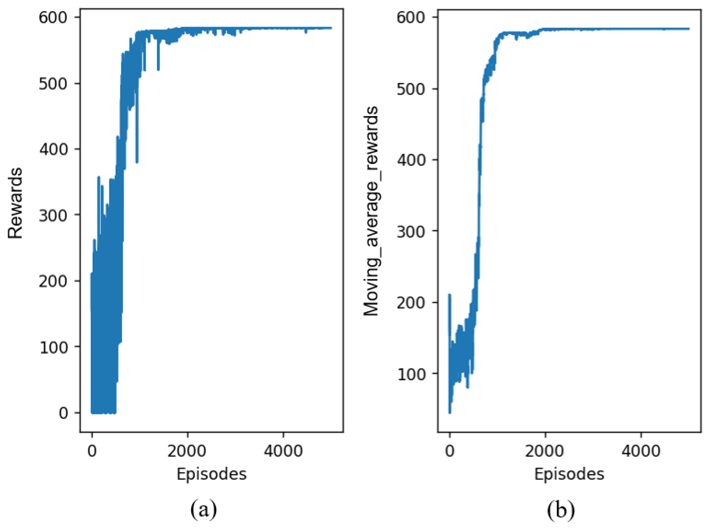
Figure 7, where
Figure 7a shows the actual episode reward curve during the training process and
Figure 7b shows the reward curve after moving average processing. It can be seen that as the number of training episodes increases, the reward keeps increasing and the performance of the agent improves significantly at around 1000 episodes, eventually converging gradually. The result shows that the training of IPPO is effective and the multiple agents learn how to choose the action so that the reward (i.e., the objective function of the model) is as large as possible.
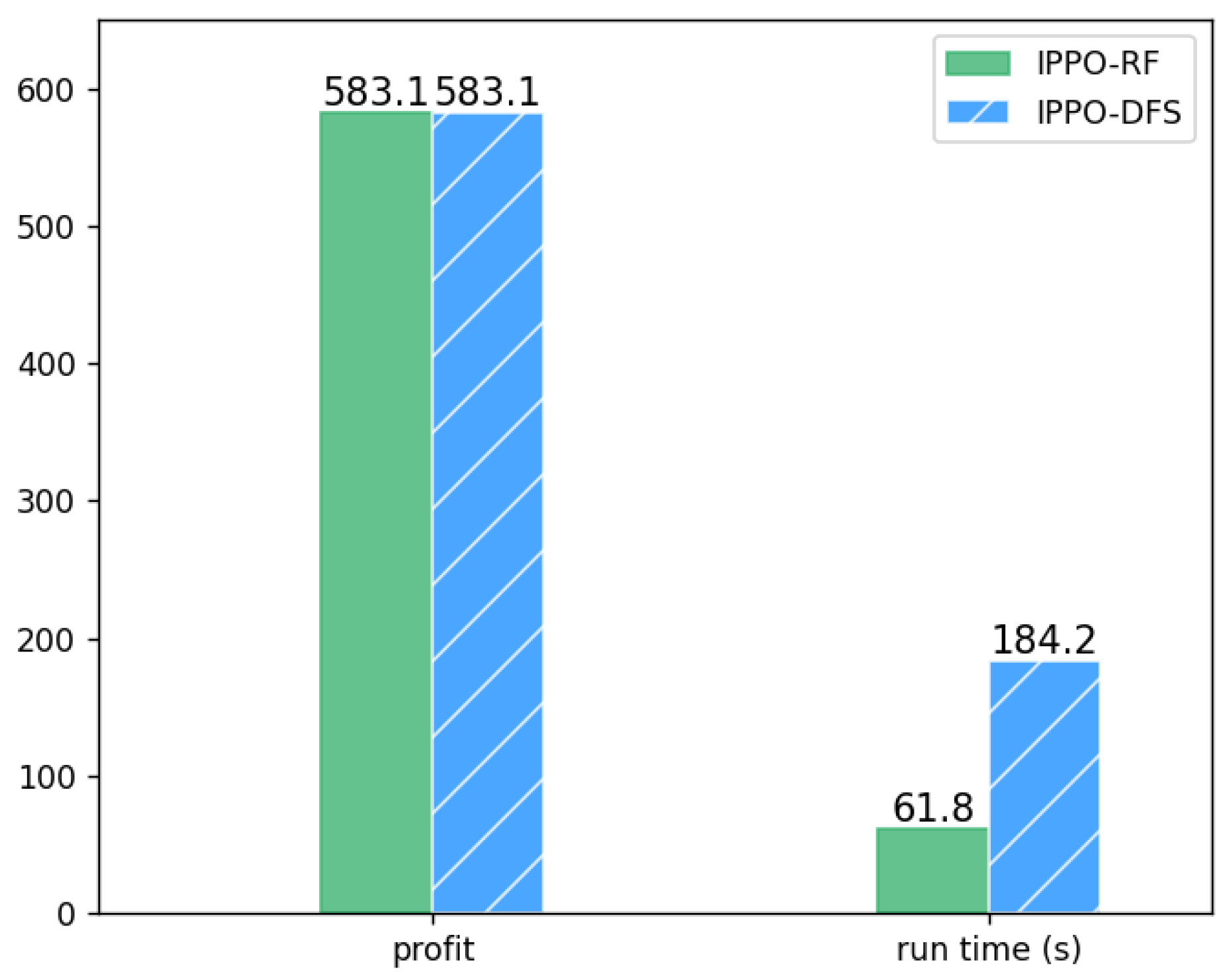
In order to illustrate the benefits of using the RF algorithm, we compare two cases. In both cases, the outer loop of finding the optimal RB allocation scheme uses the proposed IPPO method. In one case, the inner loop uses RF to determine the feasibility of the VNF mapping, denoted as IPPO-RF, and in the other case, DFS is used in the inner loop, denoted as IPPO-DFS.
The results are shown in
Figure 8, where the green bar indicates the IPPO-RF algorithm and the blue bar indicates the IPPO-DFS algorithm. It can be seen that the two algorithms obtain the approximately same profit, but the run time using RF is reduced by 198% compared to using DFS. Therefore, the RF algorithm is more efficient than the DFS algorithm in the sub-problem of verifying the feasibility of VNF mapping. This is precisely the significance of introducing machine learning into our algorithm.
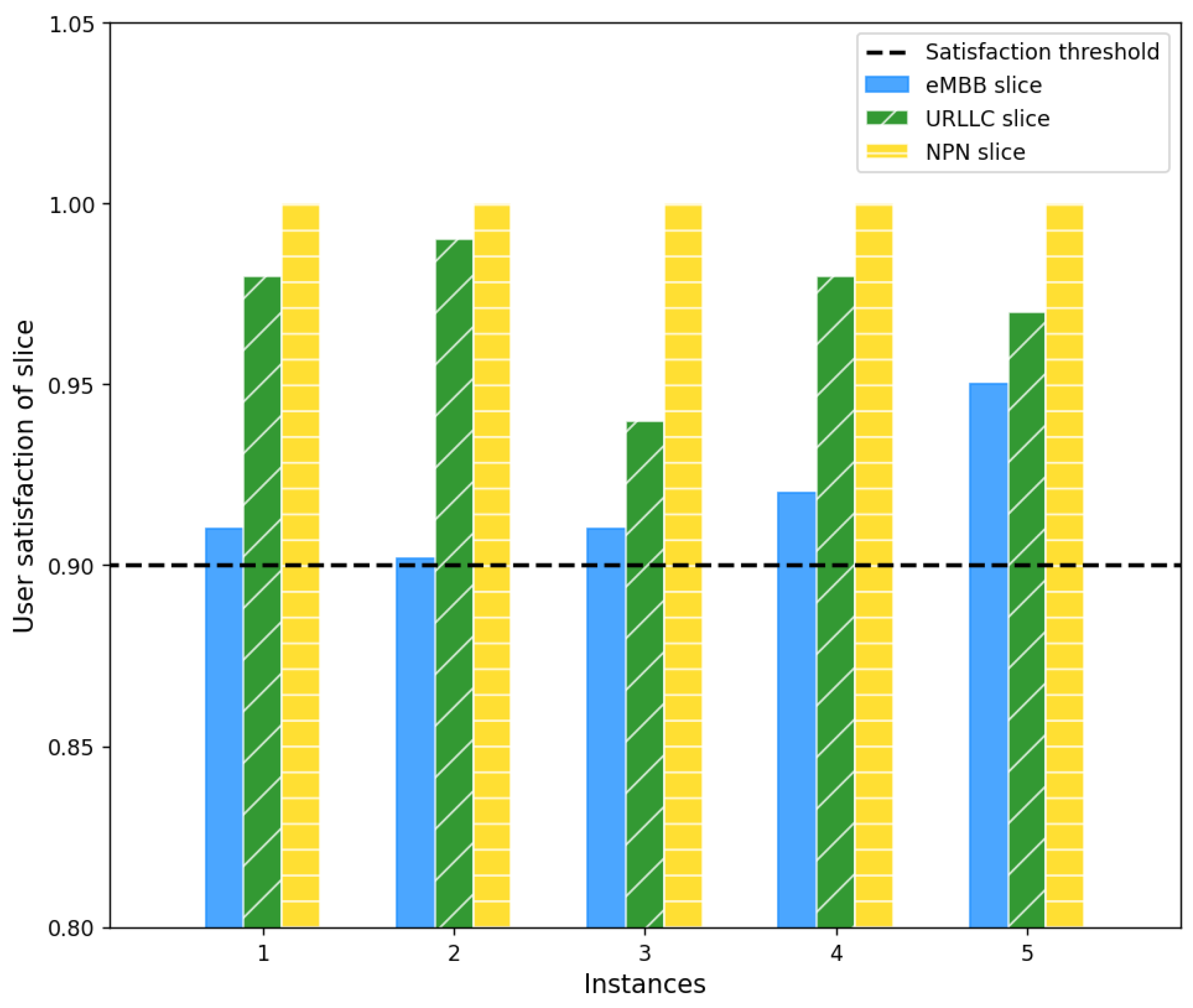
Next, we illustrate the case where the PRU is relatively large and/or the amount of resources is relatively limited, i.e., not all users can have their PRU met. We run the proposed IPPO-RF algorithm and plot the user satisfaction of the eMBB, URLLC, and NPN slices for five different instances of personalized rate requirements in
Figure 9. As can be seen, the user satisfaction of the NPN slice is always 1, which means that the higher service priority of the NPN users are guaranteed via the proposed IPPO-RF algorithm. Due to the limited resources, the user satisfaction of the eMBB slice and the URLLC slice is strictly below 1 but higher than the user satisfaction threshold, i.e.,
. Whether the eMBB slice or the URLLC slice should obtain a larger user satisfaction depends on the RB allocation scheme that can maximize the profit, and, at the same time, be implementable by a VNF mapping, and such an RB allocation scheme is found using the IPPO-RF algorithm. It can be concluded that the resource allocation scheme found via the proposed IPPO-RF algorithm does reflect that the NPN slice has higher service priority and reliability compared to the eMBB and uRLLC slices.
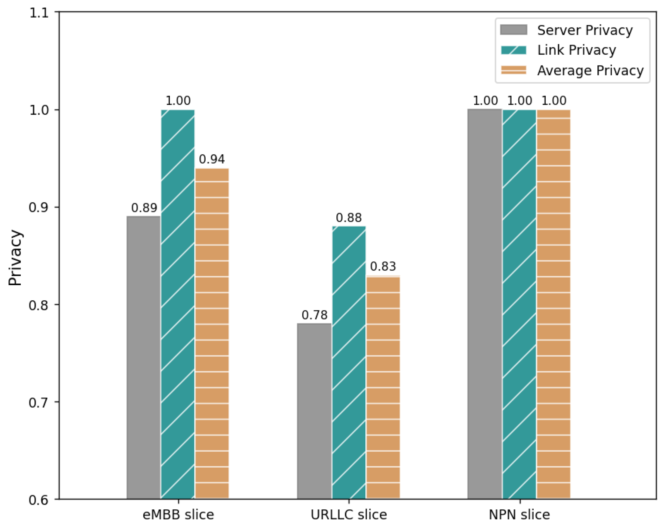
Next, we demonstrate that the RB allocation scheme found using the proposed IPPO-RF scheme can indeed guarantee the security and privacy of the NPN slices. First, we introduce three performance metrics related to the privacy of a slice: (1) the privacy of a slice on the servers; (2) the privacy of a slice on the links; and (3) the average privacy of a slice. We primarily characterize the privacy of each slice by the extent of the sharing of the servers and links occupied by the VNFs of each slice. The privacy of a slice on the servers depicts how heavily the slice shares the server nodes with other slices. More specifically, we count how many slices occupy the same server node occupied by the j-th VNF of Slice s and denote this number as . The privacy of Slice s on the servers is defined as , where denotes the computing resources required for the j-th VNF of slice s, and . Similarly, we define the privacy of Slice s on the links. Finally, the average privacy of a slice is the average of the privacy of a slice on the servers and the links.
In
Figure 10, we demonstrate the privacy of the eMBB, URLLC, and NPN slices obtained via the proposed IPPO-RF algorithm for one instance of personalized user requirements. It can be seen that the privacy of the NPN slice on the servers and links are both 1, which means that the VNFs in the NPN slice do not share server nodes or links with other slices, thus improving its security and privacy. On the other hand, the eMBB slice and the URLLC slice share some servers and links to maximize the profit. It can be concluded that the resource allocation scheme found using the proposed IPPO-RF algorithm indeed indicates that the NPN slice has higher security and privacy compared to the eMBB and uRLLC slices.
Finally, we illustrate the performance gain of the proposed IPPO-RF algorithm with three benchmark methods.
(1) Allocation in Proportion to the Personalized Requirement of Users (PPRU): First, the personalized requirement of each user or is multiplied with the minimum satisfaction threshold of the slice s and noted as . After that, the minimum RB resources required to satisfy are calculated and used as the allocation scheme for user u in slice s.
(2) Allocation by Maximizing User Rates (MUR): First, resource pre-allocation is performed to ensure that the allocated resources can meet the QoS demand of each user. After that, the remaining RBs are continuously allocated to the user with the largest rate increment and the rate increment of this user is updated. The allocation is stopped until the user satisfaction of the slice meets the requirements. Take the personalized rate requirement as an example, where the rate increment for user u is calculated as , where denotes the rate that an RB can provide to user u in slice s, and indicates the rate that the current user u has acquired. For personalized delay requirements , first convert to the rate requirements and then process them as outlined above.
(3) Allocation by Maximizing User Satisfaction (MUS): First, the same resource pre-allocation process is performed as for the algorithm MUR. After that, the remaining RBs are continuously allocated to the user with the largest satisfaction increment and the satisfaction increment of this user is updated. The allocation is stopped until the user satisfaction of the slice meets the requirements. The satisfaction increment is calculated in a manner similar to the rate increment in the MUR algorithm.
To avoid the chance of single-moment results, we change the PRU at multiple moments. First, we compare the probability of successfully completing the resource allocation for the four algorithms, randomly changing the PRU, and counting the success rate of the four algorithms in 1000 experiments. The results are shown in
Table 4. It is evident that the proposed IPPO-RF algorithm consistently provides a resource allocation scheme that meets all the requirements in every experiment. In contrast, the success rates of the remaining three algorithms are 0.42, 0.54, and 0.61, respectively, i.e., it is not guaranteed that the given resource allocation scheme satisfies all the constraints.
Then, compare the profits of the above four algorithms for five different instances when all algorithms successfully perform the resource allocation. The results are shown in
Figure 11. It can be observed that, compared to the other three algorithms, the proposed IPPO-RF algorithm can provide resource allocation schemes with higher profit. The three benchmark methods are ranked in descending order of performance as MUR, MUS, and PPRU. The proposed IPPO-RF algorithm outperforms the three benchmark algorithms PPRU, MUR, and MUS by 84%, 46%, and 57%, respectively. It can be concluded that the IPPO-RF algorithm proposed in this paper has better performance and can provide a better allocation scheme.


