1. Introduction
Managed and unmanaged grasslands provide a variety of ecosystem services [
1,
2], including provisioning services (forage production), regulating services (water and soil erosion control, agricultural pest control, soil preservation, climate stability, regulation of disease-carrying organisms, fresh water supply, flood mitigation, night cooling, and carbon sequestration), supporting services (cycling and movement of nutrients), and cultural services (aesthetic beauty). With respect to insect ecology and observed insect decline [
3,
4,
5], grasslands are vital for providing forage for herbivores and pollinators (e.g., seeds, nectar, pollen, leaves, stems, and roots), supporting habitats for insect development, and maintaining biodiversity in general. For example, in semi-natural grasslands, 25 wild plant species per 100 cm
2 can be found with an associated rich invertebrate fauna community [
6]. Insect ecology and grassland management are inextricably linked. Insects are pollinators, predators, decomposers, and food sources for other animals. They also help to regulate soil and water quality.
Agriculturally oriented grasslands are usually of reduced quality with respect to wild plant species depending on the intensity of fertilizing, plowing, re-seeding, cutting, and controlling weeds. In some cases, the original wild-plant communities have been replaced by sown monocultures of cultivated varieties of grasses and clovers such as perennial ryegrass and white clover (wikipedia.org, accessed on 15 June 2023). Trends toward intensification can be a result of changes in farming types, for example, from dairy pasture to silage production for livestock fodder or for biomass generation for biogas plants. Local changes in grassland management can lead to reduced grassland diversity at a landscape scale, negatively affecting regional insect diversity, abundance, and biomass. Statistics on agricultural practices at a national (e.g.,
www.destatis.de,
www.nass.usda.gov) or pan-national level (e.g.,
https://ec.europa.eu/eurostat) can serve as a proxy for grassland intensification analysis [
7,
8]. However, given the importance of grasslands to insect ecology and overall ecosystem health, improved measurement and assessment of grassland status at the regional and local scales are required. Corresponding systems for recent monitoring using remote sensing are currently under development at e.g., the European Space Agency, (
http://esa-sen4cap.org) and the National Ecological Observatory Network (
https://www.neonscience.org/).
A historic satellite imagery analysis provides a core technology to investigate the possible role of local grassland cultivation changes in relation to long-term insect biomass decline [
5]. We propose that annualized Normalized Difference Vegetation Index (NDVI) is a suitable proxy for annual grassland vegetation biomass with the assumption that increasing annual biomass correlates with increased grassland cultivation intensity. NDVI was designed to assess rangeland quality in the western region of the US [
9,
10] and has been used extensively since. Subsequent studies have utilized various remote sensing sensors (e.g., AVHRR, MODIS, Landsat, etc.) to continuously reinforce the use of NDVI for area estimations of biomass (among many other vegetative measurements) in grassland assessments [
11,
12,
13,
14,
15,
16].
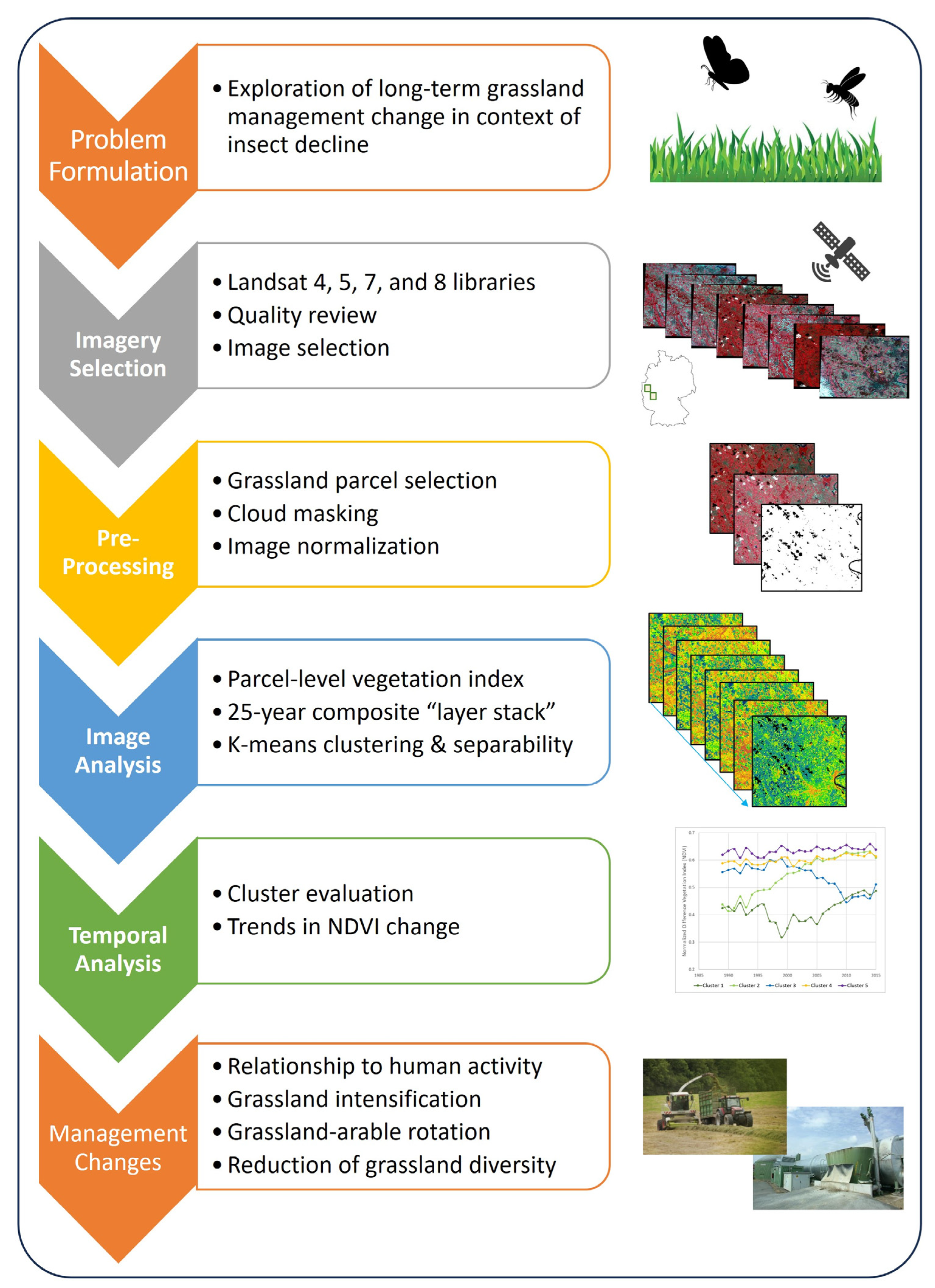
The primary aim of the current study was to characterize trends in grassland biomass change in areas where pronounced insect decline had been observed [
5]. To this end, the specific methodologic objectives of this study were to (1) determine if available imagery could be assembled and normalized to identify trends in grassland vegetation biomass over a 25-year period utilizing established approaches, (2) show that appropriate clustering of a parcel scale vegetation index (VI) could identify separable groups that illustrate differing changes in grassland management over time, and (3) place the interpretation of time series grassland changes into a context of local anthropogenic influences. The outcomes of the study are intended to provide input for the multi-factor analysis of insect decline. To our knowledge, this is the first study to develop long-term remote sensing land use change detection applied to grassland intensity for the purpose of informing insect decline research. In addition, the image normalization process applied to 100+ images is a novel combination of several established remote sensing techniques to achieve our specific study goals.
An overview of the major steps included in this article is shown in
Figure 1.
2. Materials and Methods
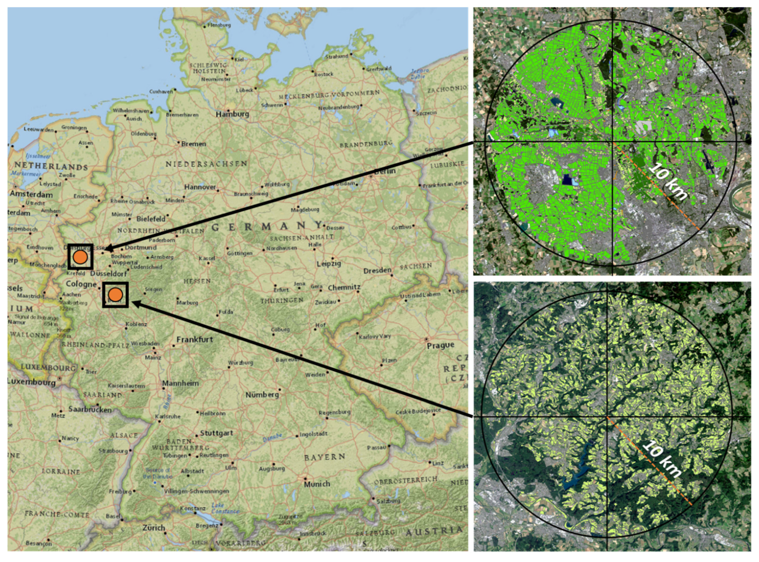
Two study sites were selected within the federal state of North Rhine-Westphalia in Germany to explore long-term changes in grassland vegetation and management using historical satellite imagery over a 25-year period. These sites were centered on several insect biomass sampling sites reported in [
5] and were identified in communication with a representative of the entomological society Krefeld (Martin Sorg, pers. comm.,
https://www.entomologica.org, accessed on 20 October 2023). Grassland parcels were characterized using several vegetation indices with the intent to cluster similar grassland parcels into groups showing distinct annual total biomass and temporal trends.
2.1. Study Sites
The first site is located in the northwest portion of Orbroich, including portions of Krefeld, a city of roughly 225,000 people on the western side of the Rhine River. The area within the Orbroich site is a mixture of developed areas along with arable land, grassland, open water, and forested areas. The second site covers Wahnbachtal approximately 25 km southeast of Cologne. Compared to the Orbroich site, the study site in Wahnbachtal contains a less densely populated, undulating landscape with small towns and includes more woods and natural grassland. The characterization of grassland change at the Wahnbachtal site was of particular interest as agricultural land use was dominated by grasslands (17% of agricultural area and 47% of agricultural parcels,
Table S1). The spatial extent of both study sites is defined by a 10 km radius which is centered on an individual insect trap location from [
5], encompassing approximately 315 km
2 (
Figure 2).
A spatial delineation of land cover parcels was performed via visual identification and classification based on high-resolution aerial imagery. Orbroich data were digitized from 64 aerial imagery tiles (10 cm resolution) from 2012/2013 obtained from Bezirksregierung Köln (
https://www.bezreg-koeln.nrw.de/, accessed on 10 June 2020), with a focus on non-developed land area (i.e., densely developed areas were not the focus of parcel digitization). A total of 17,711 parcels comprising 18,944 ha were identified as 1 of 31 land classifications using three levels of categorization (
Table S1). This study area utilized four agricultural grassland classes of meadow, meadow-orchard, silage, and other grassland as well as the neglected grassland (in total comprising 15.8% of the total parcel area (4234 parcels)). Other natural land cover classes (2130 parcels) comprised 1.4% of the total parcel area. Arable agriculture was the dominant land cover comprising 74.5% of the parcel area (
Table S1). Wahnbachtal parcels were digitized in May 2020 from high-resolution basemap imagery within ESRI’s ArcGIS Online platform. Parcel digitization for Wahnbachtal was focused on grassland only (
Figure S2). This resulted in 3256 parcels comprising 7548 ha with an average parcel size of 2.3 ha (
Table S2).
Grassland polygons were subsequently reviewed to remove parcels that were too small or narrow for appropriate characterization based on a 30 m resolution of the satellite imagery. This selection process only included polygons with a minimum size of 0.4 ha and an area-to-perimeter ratio >10 (which eliminated the long narrow and oddly shaped polygons). The remaining polygons were buffered inward by 30 m to reduce the potential for mixed pixels to be included in the analysis and rasterized in alignment with the satellite imagery (
Figure S3). After this pre-processing of the input parcels, a final set of grassland polygons remained composed of 818 polygons for Orbroich and 1367 polygons for Wahnbachtal.
2.2. Satellite Imagery Selection
Archive imagery from the NASA/USGS Landsat program (
https://landsat.gsfc.nasa.gov/, accessed on 12 March 2020) was reviewed to identify potentially suitable images from the Thematic Mapper (TM) sensor covering some or all of the study site area in the time period of 1989 through 2013 (Orbroich) or 2015 (Wahnbachtal). Given the extended length of this analysis, imagery from Landsat 4, 5, 7, and 8 were all considered as potential sources, with images from Landsat 5, 7, and 8 selected. TM image data are composed of seven core spectral bands starting with Landsat 4 (although more bands were added to subsequent satellites) ranging from visible blue (0.45–0.52 µm) to short-wave infrared (2.08–2.35 µm) at a 30 m ground resolution. These data also include a thermal band (10.40–12.50 µm) at a 60 m resolution that was not used in our analysis.
The presence of clouds during image acquisition impedes the usefulness for optical image analysis as clouds and haze (and their associated shadows) can drastically affect the reflection of some electromagnetic wave energy from the surface of the earth. Images were divided into quadrants and filtered based on a ruleset where images exceeding a threshold of cloud cover were removed from consideration during the review process. In total, 166 Level-1 images (i.e., raw digital numbers (DNs) and not atmospherically corrected) were selected and downloaded for the Orbroich site and 266 images for the Wahnbachtal site. The number of images available across years and seasons varied (
Table S3). A detailed assessment of image quality was performed, including georeferencing accuracy/image-to-image registration, a more detailed cloud cover assessment, and overall spectral data quality. Details of this assessment are provided in
Supplementary Materials.
2.3. Image Normalization
To obtain the best results when comparing spectral information received at the sensor across different acquisition dates, the data should be converted from their original digital number format into a meaningful physical unit (e.g., percent reflectance). This type of conversion process, often referred to as radiometric calibration, allows for these remotely sensed data to be compared across both time and space. Other studies have used an image normalization process in lieu of radiometric calibration [
17,
18,
19] to achieve image comparability across time and space. Due to the data volume and the potential for unverifiable error in generating radiometrically calibrated data from models reliant on historic atmospheric information over 25 years, this study implemented a robust method to normalize the data for spatiotemporal comparability. The process minimizes differences from one date to another due to atmospheric variations (e.g., sun elevation, sun intensity, atmospheric attenuation) on different dates of acquisition.
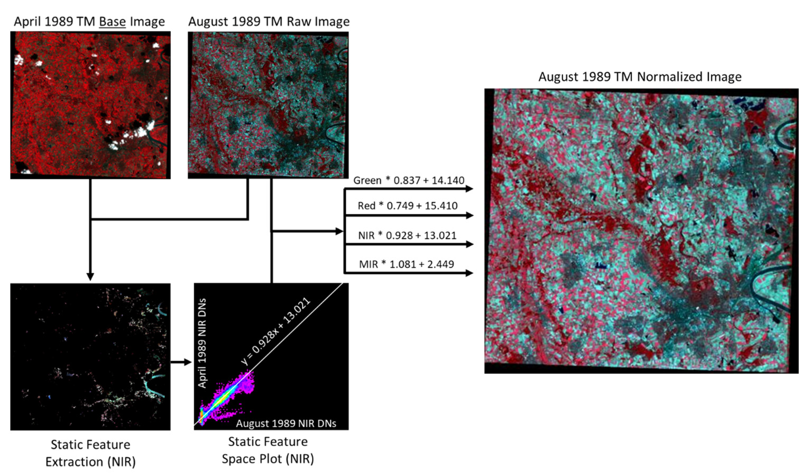
This image normalization involved the creation of a mask that included features with little or no spectral variation over time (i.e., non-vegetation features such as asphalt, concrete, roofs, water, bare soil) within a base image. Spectral information from the same features in a second image was compared to that of the base image using a feature space plot displaying three dimensions of information: (1) the base image spectral band values on the
y-axis; (2) the second image spectral band values on the
x-axis; and (3) the color-ramped plot of pixel frequency (
Figure S4). From these plots, a linear regression for each spectral band was developed from the soil/static feature line that passed through the feature space plot using the ordinary least squares (OLS) method. The band-specific linear regressions were used to scale all pixels in the second image to the base image in order to normalize the data, enabling a pixel-to-pixel comparison across time and space.
Figure 3 illustrates this approach where NIR pixel values from locations of multi-date static features in a base image (April) and non-base image (August) were combined in a feature space plot, with the generated linear regression. The regression equation, along with similarly generated regressions for the green, red, and mid-infrared (MIR) bands, was applied to all pixels in the August image to normalize the data for any differences in atmospheric conditions between acquisition dates.
To accomplish this normalization for hundreds of images, a two-stage method was implemented. In stage one, a single image from each year (light orange column in
Figure S5) was normalized to a master base image (April 1989, dark orange in
Figure S5) to minimize interannual variation and produce a base image for each year of the study adjusted to 1989. The annual image selected for normalization was most consistent in time of year with the master base image, ranging from March to June, with the majority coming from April. In the second stage, images were normalized for all months within a single year to the base image of that year to minimize the intra-year variation of static features (e.g., each row in
Figure S5). The application of this methodology resulted in a 25-year chronology of 166 (Orbroich) or 266 (Wahnbachtal) images where the variation of spectral information within each parcel was, as much as possible, due to potential changes in land use. Further details of this methodology are provided in
Supplementary Materials.
2.4. Vegetation Indices
Vegetation indices (VIs) use the characteristics of two or more bands of wave energy reflecting from vegetation surfaces in which reflection/absorption is influenced by physical aspects such as plant structure, pigment type, nutrient deficiencies, and moisture content. Many VIs include the red visible wavelengths (strongly absorbed by plant chlorophyll) and the near-infrared wavelengths (unaffected by chlorophyll but highly reflected in a healthy plant structure). The difference in response to vegetation in these two wavelengths has been used for nearly 50 years to monitor vegetation health. There is a long history of using NDVI for vegetation-related studies [
9,
10], and many use NDVI as an indicator of vegetation biomass [
11,
12,
13,
14,
15,
16,
20,
21,
22,
23]. Additional VIs were considered for use in this study (see
Supplementary Materials); however, NDVI was chosen because of the long and well documented history of this vegetation index.
NDVI was calculated for each pixel in each grassland parcel for every image date (multiple images per year over multiple years). Parcel-wide statistics were computed (mean, minimum, maximum, standard deviation, and count) to address within-parcel variation and used as the basis for the subsequent clustering process. Individual date and mean annual NDVI statistics were computed for each year.
2.5. Grassland Parcel Clustering
To identify patterns of biomass change indicated by NDVI, grassland parcels were grouped into a distinct set of clusters using a k-means minimum distance algorithm. This iterative process using NDVI statistics resulted in four clusters of grassland polygons for Orbroich and five clusters in Wahnbachtal. The parcels in the clusters were grouped based on the clustering algorithm’s mathematical principle of minimizing the within-class variation, while at the same time maximizing the between-class variation. The test of cluster uniqueness was verified through separability analysis using Transformed Divergence (TD) [
24].
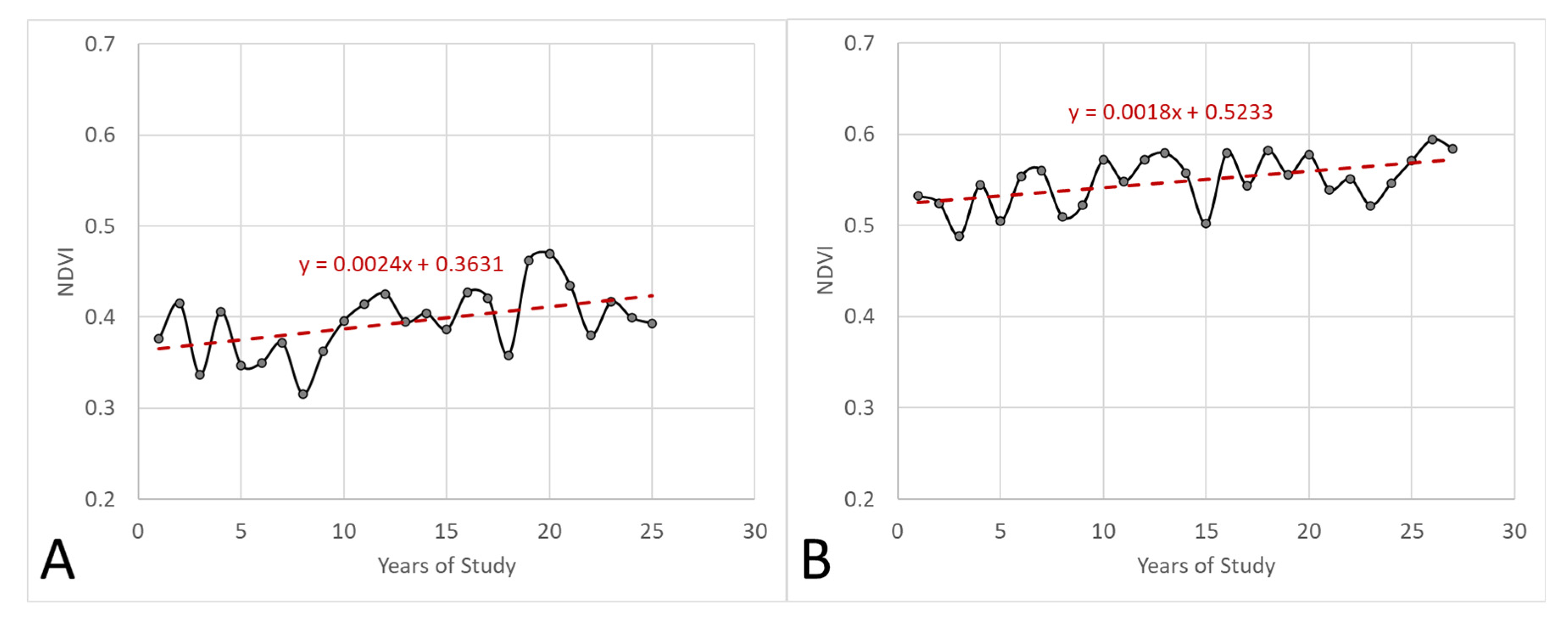
There are a variety of factors related to climate and surface-level conditions that may introduce temporary, short-term changes in reflectance values captured by satellite imagery that may be inconsistent with the long-term trajectory. For example, a drought during one year would reduce vegetation vigor (lower NDVI) and biomass compared to the previous or subsequent year. Likewise, a particularly cold or warm winter could influence the timing and amount of vegetation during springtime. To address these year-to-year variations that may confound trend analysis, the mean NDVI for all clusters was computed for each year, and a linear model was used to generate the residual from the mean for each combination (
Figure 4). This residual adjustment was applied to each individual cluster/year combination [
25] (
Figure S6). The adjustment for single-year events affecting annual biomass allowed for a clearer picture of temporal trends between clusters.
Additional sub-clustering was completed on the set of five clusters from Wahnbachtal to determine if subclasses existed that could potentially reveal valuable temporal trends in grassland characteristics. The subcluster analysis typically violates the assumptions related to separability [
26]; however, sub-clustering can often reveal interesting patterns that can add value to trend analyses. To further explore the influence of averaging the NDVI values for a grassland parcel over 12 months, a base-image (spring/early summer) NDVI clustering process was performed. Methods and results are reported in
Supplementary Materials.
3. Results
A total of 818 grassland parcels encompassing 1655 ha were grouped into four distinct clusters for the Orbroich study site, with parcel counts per cluster ranging from 123 to 340 (15.5% to 43.2% of total grassland area). In Wahnbachtal, five clusters were identified for the 1367 grassland parcels (5083 ha), with parcel counts per cluster ranging from 65 to 598 (4.8% to 43.7% of total grassland area) (
Table 1). The separability of clusters was confirmed using TD measurements between cluster pairs, where results of 1900 or larger indicate a high separability between cluster pairs [
26]. The Orbroich site had an average TD of 1958 (only one of the six pairwise combinations was <1900); the Wahnbachtal site had an average TD of 1962, and all pairwise comparisons were greater than 1900, except one combination (
Table 1). This indicates that the majority of individual clusters were statistically separable (TD > 1900) from one another based on their temporal patterns in VI values. The exceptions to very high separability were in cluster pair 3:4 in Orbroich and cluster pair 4:5 in Wahnbachtal. Even these values (1802 and 1621, respectively) could be considered to have adequate separability based on [
27] who used a threshold of 1700 as good separation and 1500 as adequate. In both cases, these cluster pairs represented similar temporal patterns of consistently high NDVI values over the course of the study period but allowed for the separation from the other clusters. An additional analysis of the resulting clusters and separability is provided in the SI. An evaluation using TD was also performed on alternate VIs investigated (see
Table S5 in Supplementary Materials).
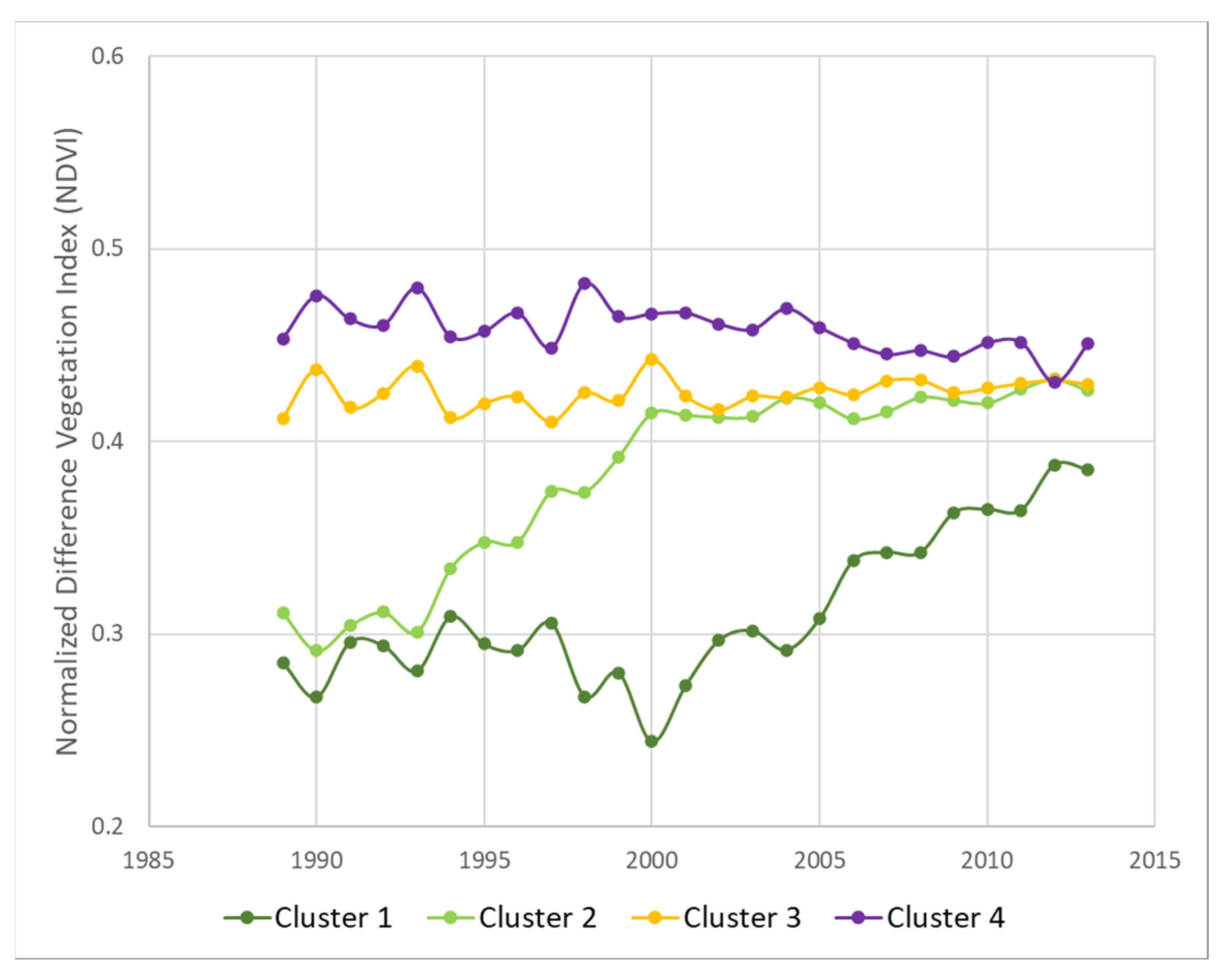
NDVI results for each cluster are composed of 25 annual values based on the average of the grassland parcels within the cluster for that year (
Figure S6, left). Large-scale events occurring in one year that may cause a shift in vegetation compared to other years (e.g., drought, early warm weather) were smoothed using a linear regression that was calculated from the average of all clusters for each year (
Figure 5 and
Figure S6, middle). The difference between the average of all clusters for each year relative to the linear regression equation was used to adjust each cluster’s original yearly value. This was performed for each NDVI cluster value for each year to generate the final annual NDVI values for each cluster (
Figure 5 and
Figure S6, right).
Figure 5 displays the temporal sequence of annual mean NDVI for each cluster of grassland polygons in Orbroich, where three distinct patterns emerge in grassland biomass (as described by NDVI). Clusters 3 and 4 (orange and purple) remain fairly constant over 25 years although at different NDVI levels. Cluster 2 (light green) starts to increase in biomass in the mid-1990s, reaching the levels of Clusters 3 and 4 around year 2000. Cluster 1 (dark green) remains fairly constant until the early 2000s and then increases to almost the level of the other clusters by 2013. Based on these trends, the diversity of grassland conditions could be considered to have decreased within the 25 years as described by the narrowing NDVI (biomass) range between clusters.
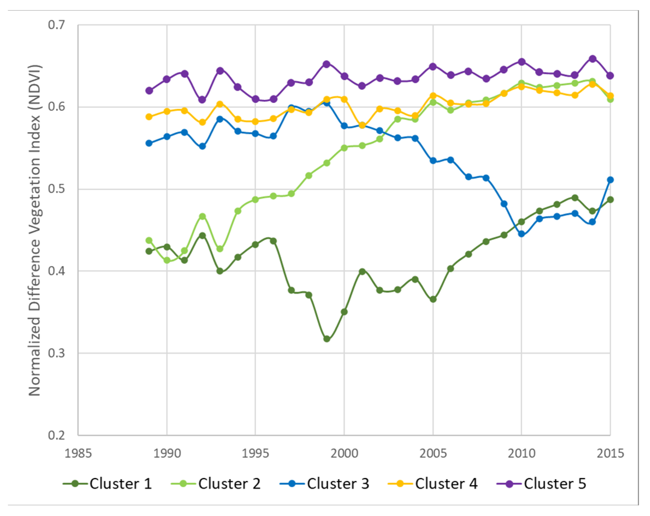
Similar patterns can be observed in Wahnbachtal (
Figure 6), with the two highest NDVI clusters (4 and 5, orange and purple) remaining fairly constant between 1989 and 2015. A trend that is not present in the Orbroich site is Cluster 3 (blue). This cluster has a constant high NDVI similar to Clusters 4 and 5 until about year 2000, but it has a period of decline to 2010 and then tracks closely with Cluster 1 (dark green). Parcels in Cluster 2 (light green) exhibit increasing biomass starting in the early 1990s and match the high-biomass clusters around 2005. Cluster 1 (dark green) remains relatively constant up to about 2005 and then increases to 2015.
The time series plots for each site are comparable in their temporal patterns; however, caution should be used when comparing NDVI values across sites. Each of the two study sites used a different 1989 base image for normalization; therefore, these were independent analyses of the clusters’ temporal trends.
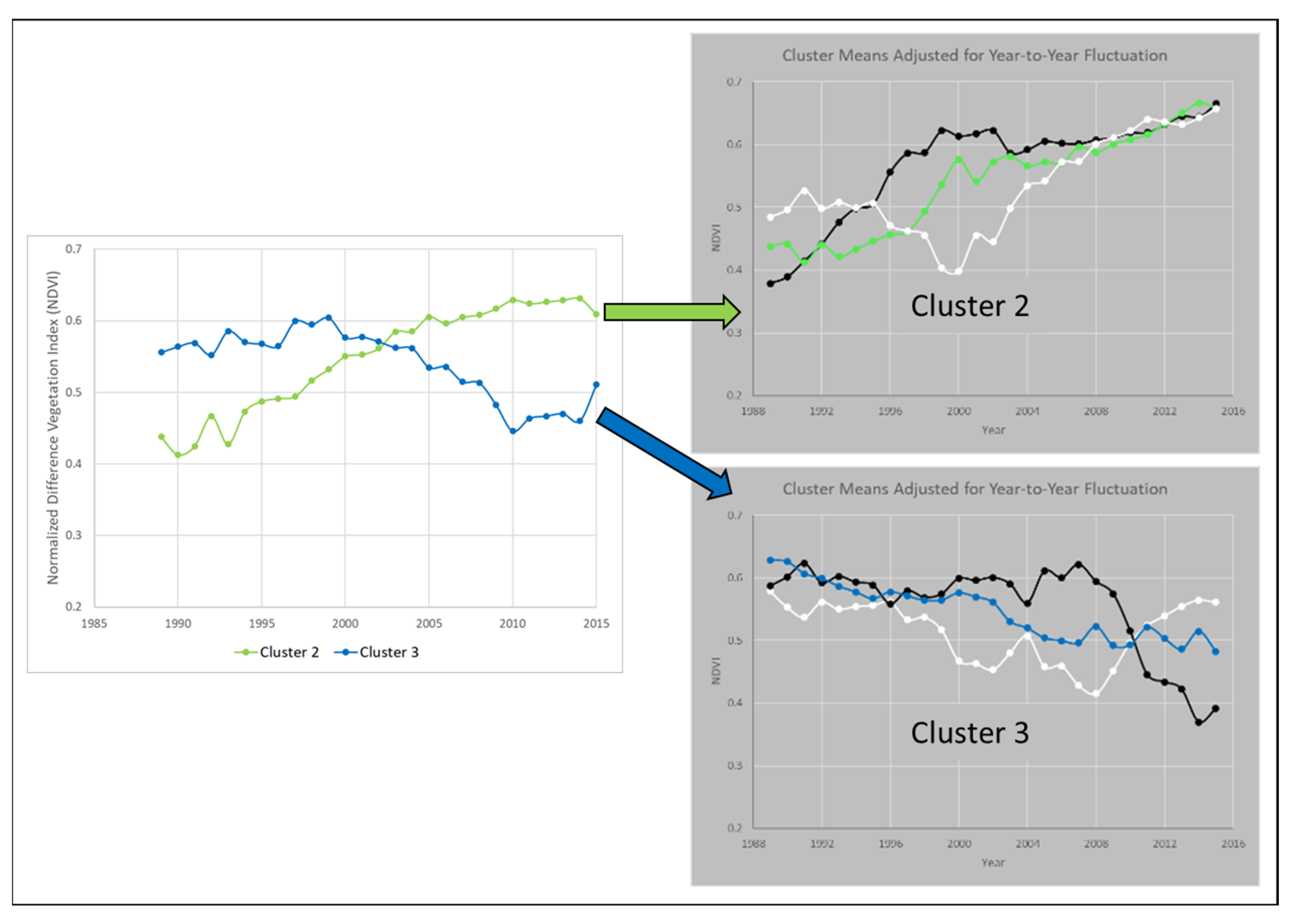
An additional analysis of all Wahnbachtal clusters was performed using a sub-clustering approach to explore further temporal trends within the main clusters. For example, the analysis of two highly separable clusters (TD = 2000) in Wahnbachtal (Clusters 2 and 3, light green and blue) revealed additional temporal patterns indicating that each of the resulting subclusters initiates changes in NDVI at different time periods (
Figure 7). All subclusters followed the same increasing or decreasing trend as the primary cluster over the 25 years; however, the timing of the increase or decrease differed between the subclusters.
An analysis of within-cluster variability over time was performed by plotting the standard deviation of the annual average NDVI for all grassland polygons within a cluster for each year. This demonstrated that cluster variability (i.e., standard deviation of individual grassland parcel NDVI values) was low and stayed consistent for Clusters 3 and 4, decreased for Cluster 2, and was high but somewhat variable for Cluster 1 for Orbroich (
Figure S9). For Wahnbachtal, cluster variability was also low for Clusters 4 and 5, increasing for Clusters 1 and 3, and decreasing for Cluster 2 (
Figure S10). An increase in total parcel biomass coupled with a decrease in biomass variability within a cluster over time (e.g., Cluster 2 in both Orbroich and Wahnbachtal) indicates lower spatial and temporal diversity. This could be the result of the increasing management intensification of grassland habitats in these areas, with possible related reductions in insect abundance.
4. Discussion
We identified four distinct clusters of grassland parcels with biomass trends over 25 years for the Orbroich site. While two clusters remained relatively constant at high NDVI levels, the other two clusters showed marked increases in annual vegetation biomass over time, reaching or nearing the “constant” clusters by 2013. For the two increasing biomass clusters, the starting year of increase occurred at different times. By 2013, grassland conditions were less diverse compared to 1989. Several anthropogenic factors may be related to these increases. There has been a decrease in dairy farming in the area coupled with an increase in silage production [
28]. This shift from extensively managed grassland (i.e., dairy pasture) to intensive silage grassland may in part explain the trends identified. Additionally, the number of biogas generation plants increased significantly between 2000 and 2017 with the Renewable Energy Sources Act [
28]. Across Germany, the area of silage maize for biogas increased by approximately 700,000 ha between 2007 and 2018 [
28,
29], which overlaps the timeframe of the increasing NDVI of Cluster 1 for both Orbroich and Wahnbachtal. Grasses and other silage crops are more intensively managed to generate additional biomass for conversion to biogas.
In Wahnbachtal, five clusters were identified with two clusters having a relatively constant annual average biomass, two clusters with an increasing biomass, and one cluster with a decreasing trend (
Figure 5). A preliminary evaluation examined generalized changes in grassland parcels over time using Google Earth time series imagery. This evaluation indicated that Clusters 1 and 3 were a temporal mixture of grassland and arable uses over the time period. Cluster 1 primarily had early changes from arable to intense grassland uses and Cluster 3 parcels changed from early grassland use to mixed use (e.g., silage, arable, grassland combinations). The parcels in the two temporally constant clusters (4 and 5) have likely been continual pasture and/or meadow (hay) uses over the time period with no mix of arable crops during those years. Parcels examined in Cluster 2 (which had a large increase in biomass over time) also had little or no mixing with arable uses; however, the intensity of grassland use increased over time (e.g., change from pasture to intense meadow (hay) or silage production). This cluster also included some parcels permanently changed from arable to grassland within the 25-year window (but not fluctuating back and forth). Cultural changes in this area from 1989 to 2015 include the addition of nearby biogas plants and an increase in recreational horse riding and farming. These factors may affect grassland management practices to intensify biomass production for biogas or silage.
Although distinct clusters of grassland parcels with clear trends over time were observed, there were additional factors influencing the results that should be considered. These factors are listed below and discussed in
Supplementary Materials:
Designation/definition of grassland polygons;
Satellite image selection and pre-processing;
Satellite image normalization;
Use of NDVI as a proxy for biomass;
Temporal aspects of metrics for grassland parcel characterization;
Within-cluster similarity.
The integration of more than one hundred satellite images spanning several decades into a single spectrally normalized time series and the subsequent analysis method used are not limited to the specific locations presented here. This investigation on grassland change and local insect abundance is transferable and can be applied to other geographic regions. This could include other locations observed in the insect study of [
3,
4,
5], and other studies [
30]. However, the interpretation of the temporal trends and their correlation to environmental changes in the landscape will differ depending on the area being studied. In addition, more specific grassland intensification indicators can be derived and applied to assess (bio)diversity loss related to intensification and monoculturalization at larger geographic regions, such as those used as foundational information to reach future sustainability goals (e.g., EU Green Deal (
https://ec.europa.eu/info/strategy/priorities-2019-2024/european-green-deal_en, accessed on 26 July 2023) and EU Farm-to-Fork (
https://ec.europa.eu/food/system/files/2020-05/f2f_action-plan_2020_strategy-info_en.pdf, accessed on 26 July 2023)).


 ,
, 
