
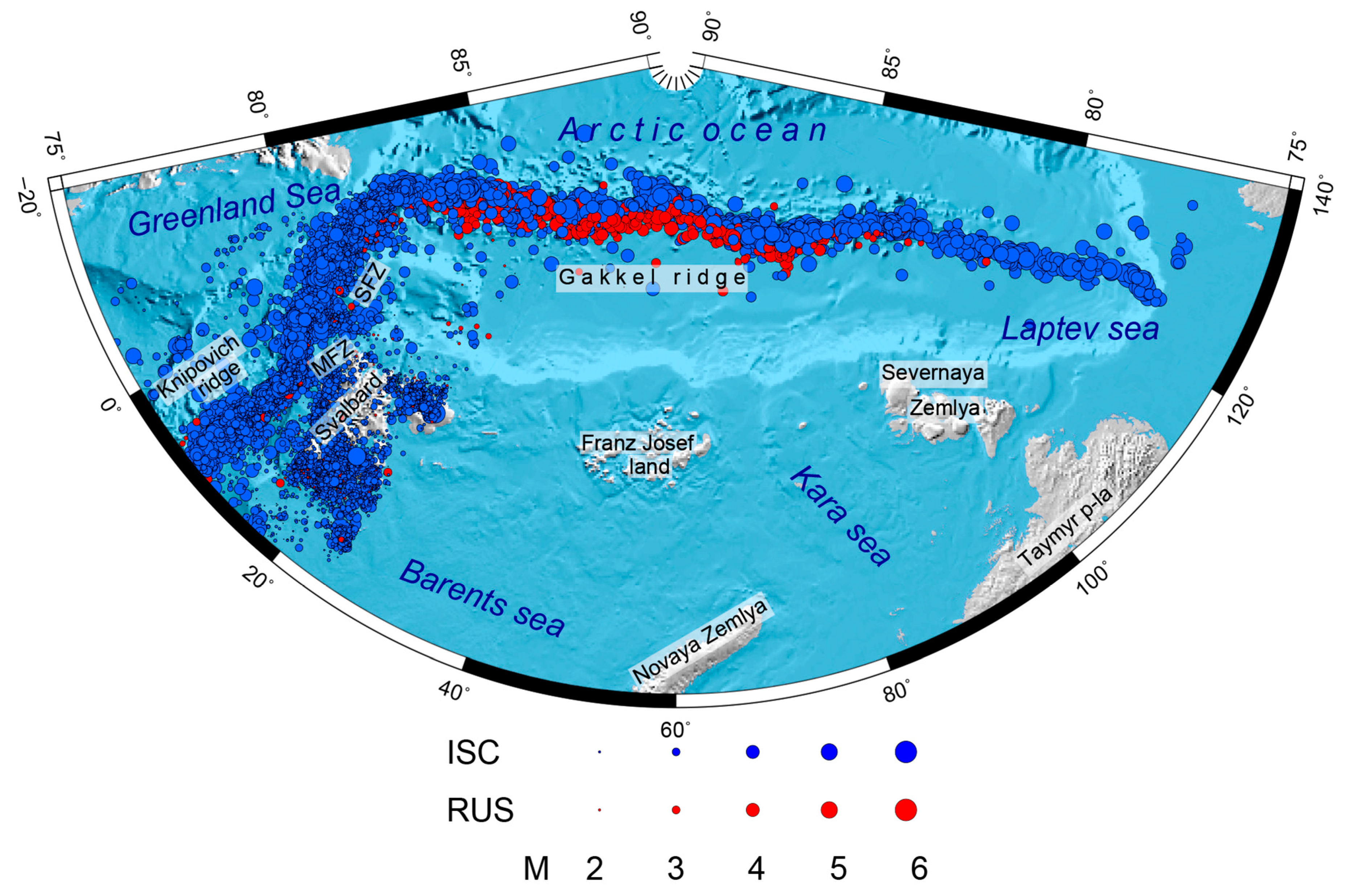
Integrated Earthquake Catalog III: Gakkel Ridge, Knipovich Ridge, and Svalbard Archipelago


 ,
,  , , and
Abstract
1. Introduction
2. Materials and Methods
- The Arctic catalog from the annual journals Earthquakes in the USSR 1962–1991, Earthquakes in Northern Eurasia 1992–2017, and Earthquakes in Russia 2018–2021 (hereinafter ARC);
- The catalog of the FCIAR network (Arkhangelsk network) 2008–2017 from the annual journals of Earthquakes in Northern Eurasia (hereinafter ARKH);
- The catalog of the Svalbard Archipelago territory for 2010–2021 from the annual journals of Earthquakes in Russia (hereinafter SHB);
- The ISC 1962–2022 catalog, which is a composite and contains data from many world and also Russian agencies (Table S1, see Supplementary);
- The catalog Seismicity of the western sector of the Russian Arctic for 1962–2020 [29] (hereinafter Morozov). The Morozov catalog was recently presented in [29]. In this catalog, earthquakes are relocated based on the analysis and merging of all available seismic bulletins from Russian and European seismic networks using modern velocity models. The Morozov catalog covers the shelf zone of the Western Sector of the Russian Arctic, which we included in our previous study [28], but some earthquakes were relocated [29] from the shelf to the Gakkel Ridge. We include these events in our catalog, since we consider determinations [29] to be the most reliable.

| Catalog | Period | Number of Events | Number of Earthquakes with Energy Classes and/or Magnitudes | Number of Non-Earthquakes |
|---|---|---|---|---|
| ARC | 1965–2021 | 2404 | 2403 | 1 * |
| ARKH | 2008–2017 | 1493 | 1492 | 1 * |
| SHB | 2010–2021 | 2634 | 2634 | 0 |
| ISC | 1962–2022 | 16,953 | 16,937 | 16 |
| Morozov | 1962–2020 | 4 ** | 4 | 0 |
3. Results
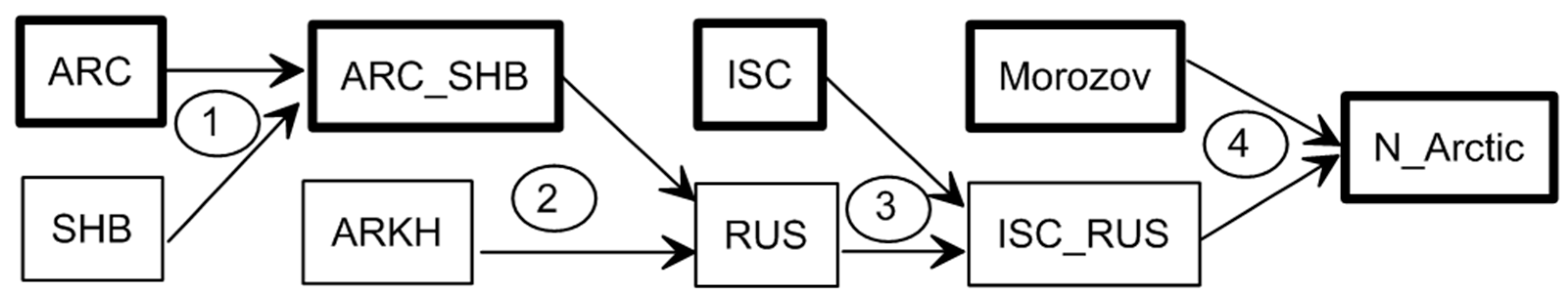
3.1. Merging Catalogs
- Earthquakes from the Morozov catalog (4 events);
- Earthquakes from the ISC catalog (16,937 events);
- Earthquakes from catalogs of ARC (2404 events), SBH (2404 events), and ARKH (1493), with preference given to data from the ARC catalog in overlapping areas.

| Stage | Main Catalog | Additional Catalog | km | Threshold Value of the Metric | Estimation of the Number of Errors | Number of Duplicates | Merged Catalog |
|---|---|---|---|---|---|---|---|
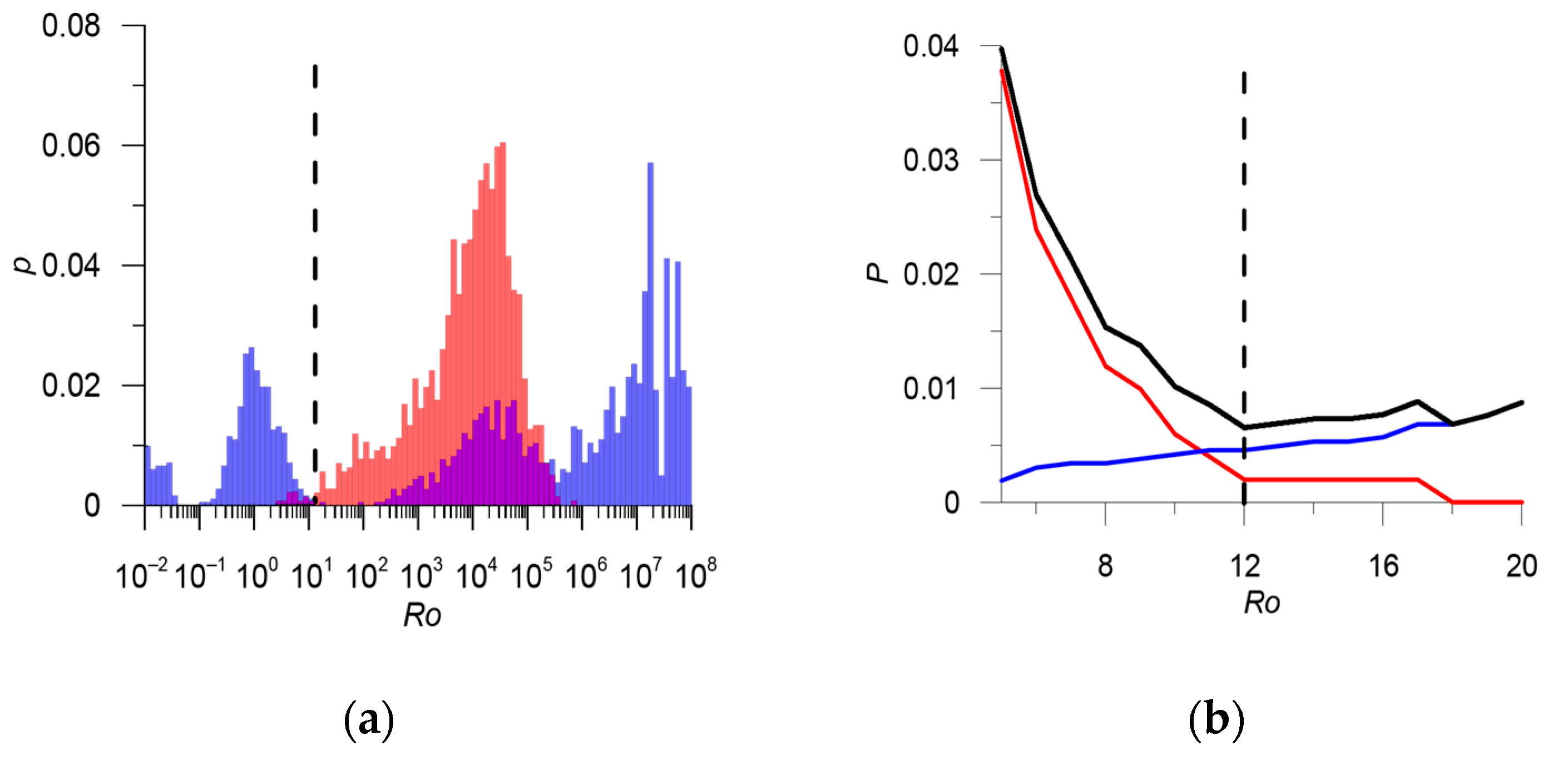
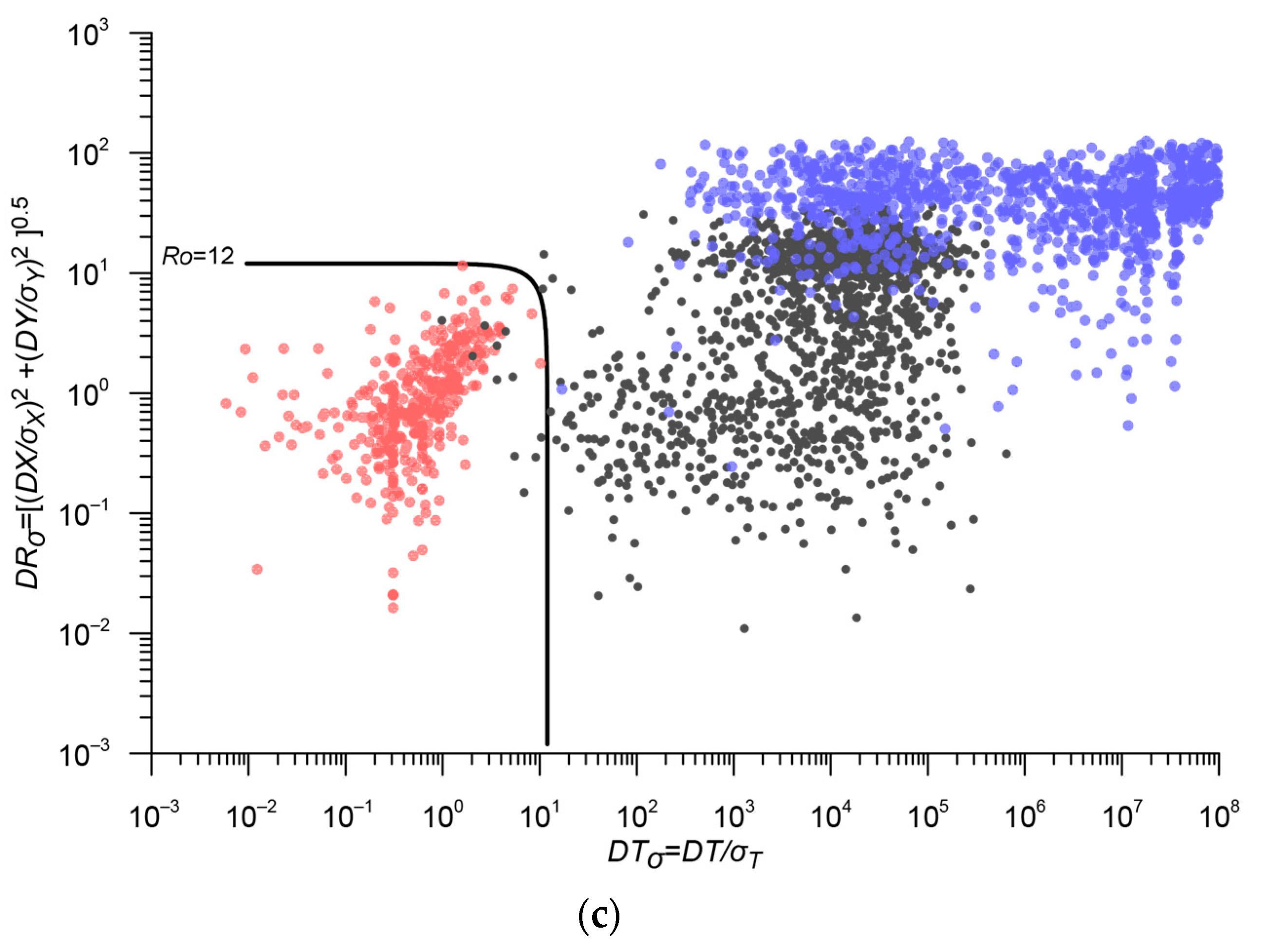
| 1 | ARC 2403 events | SHB 2634 events | 0.054; 22.5; 21.3 | 12 | 0.7% | 502 | ARC_SHB 4535 events |
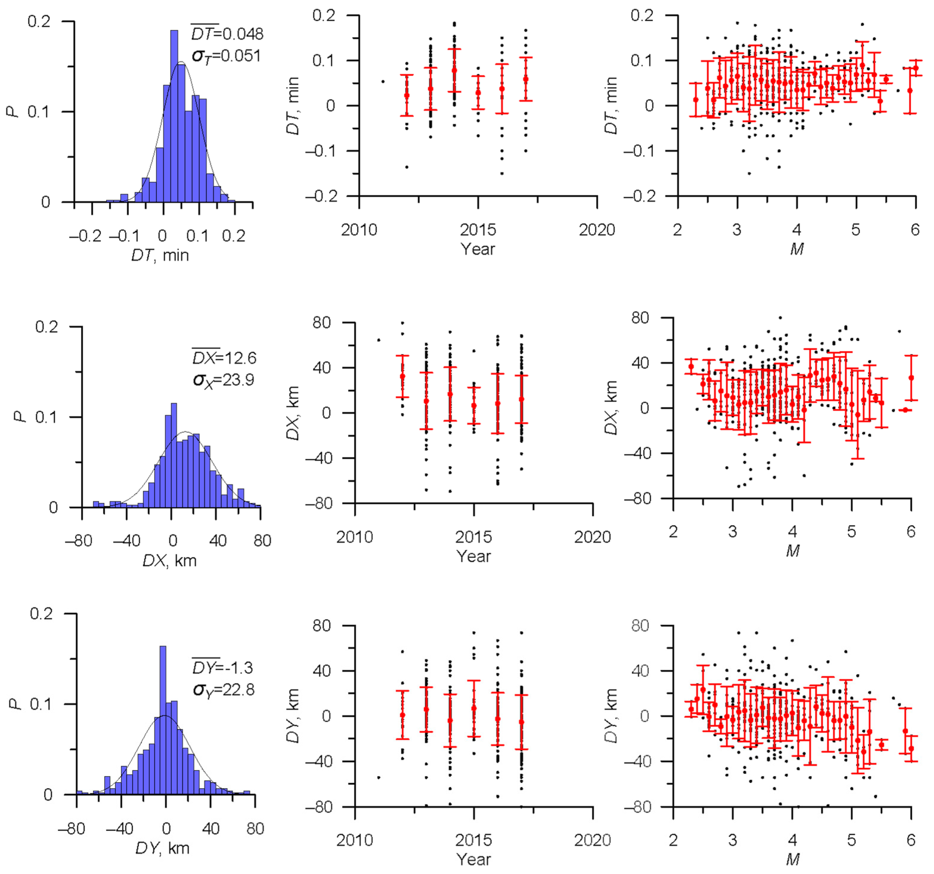
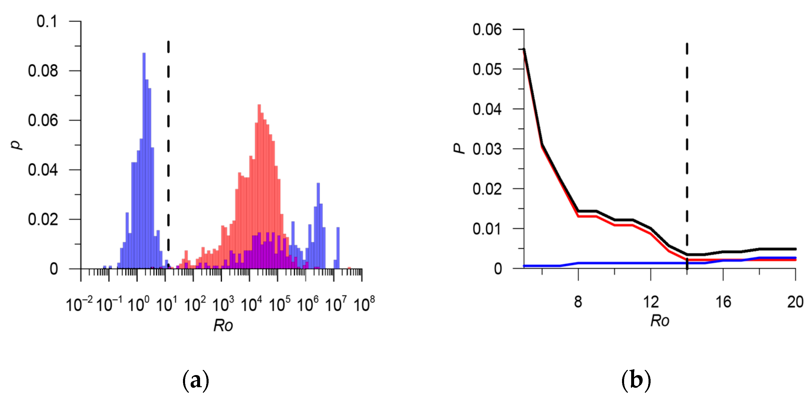
| 2 | ARC_SHB 4535 events | ARKH 1492 events | 0.048; 23.9; 22.8 | 14 | 0.3% | 1136 | RUS 4891 events |
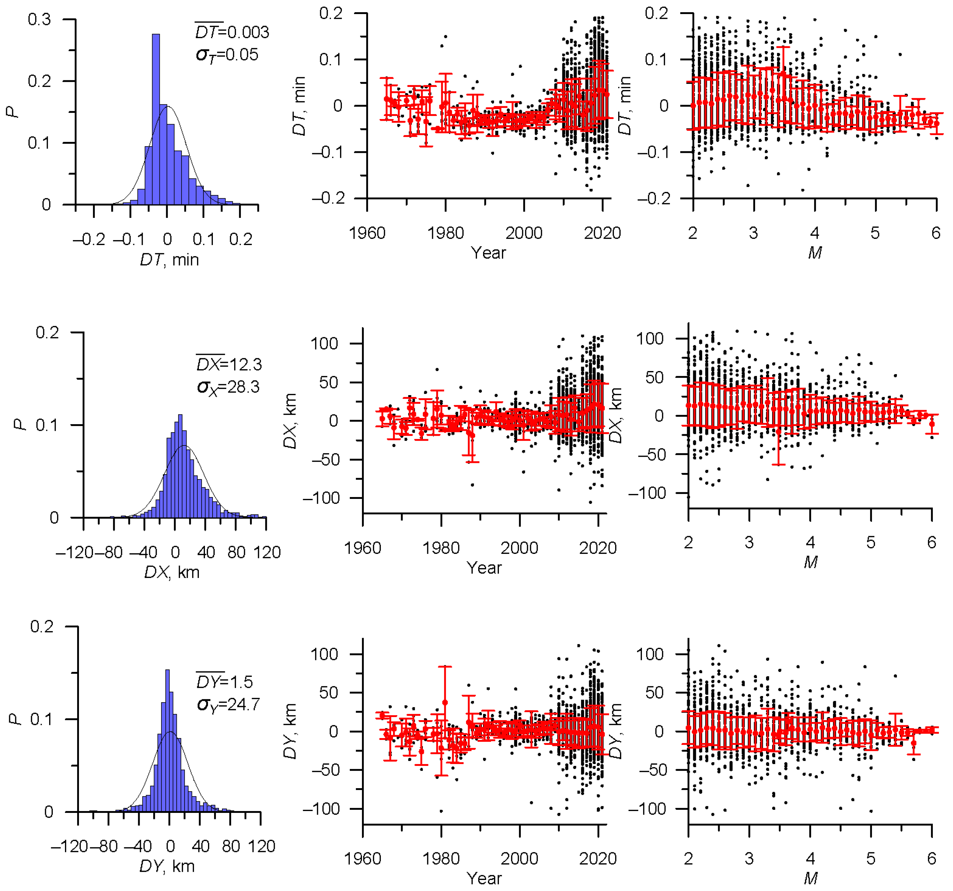
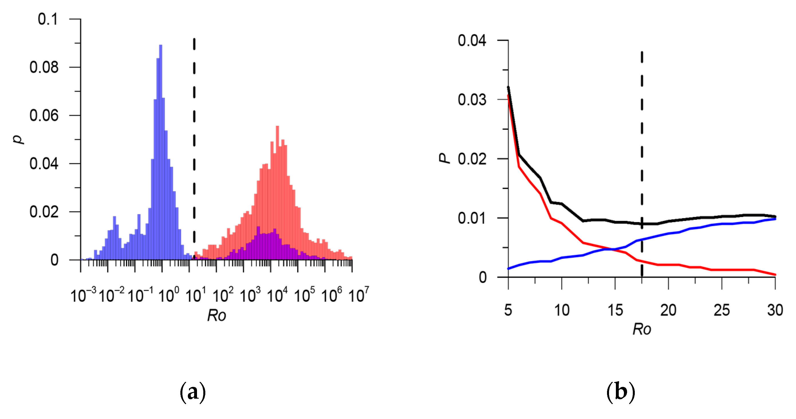
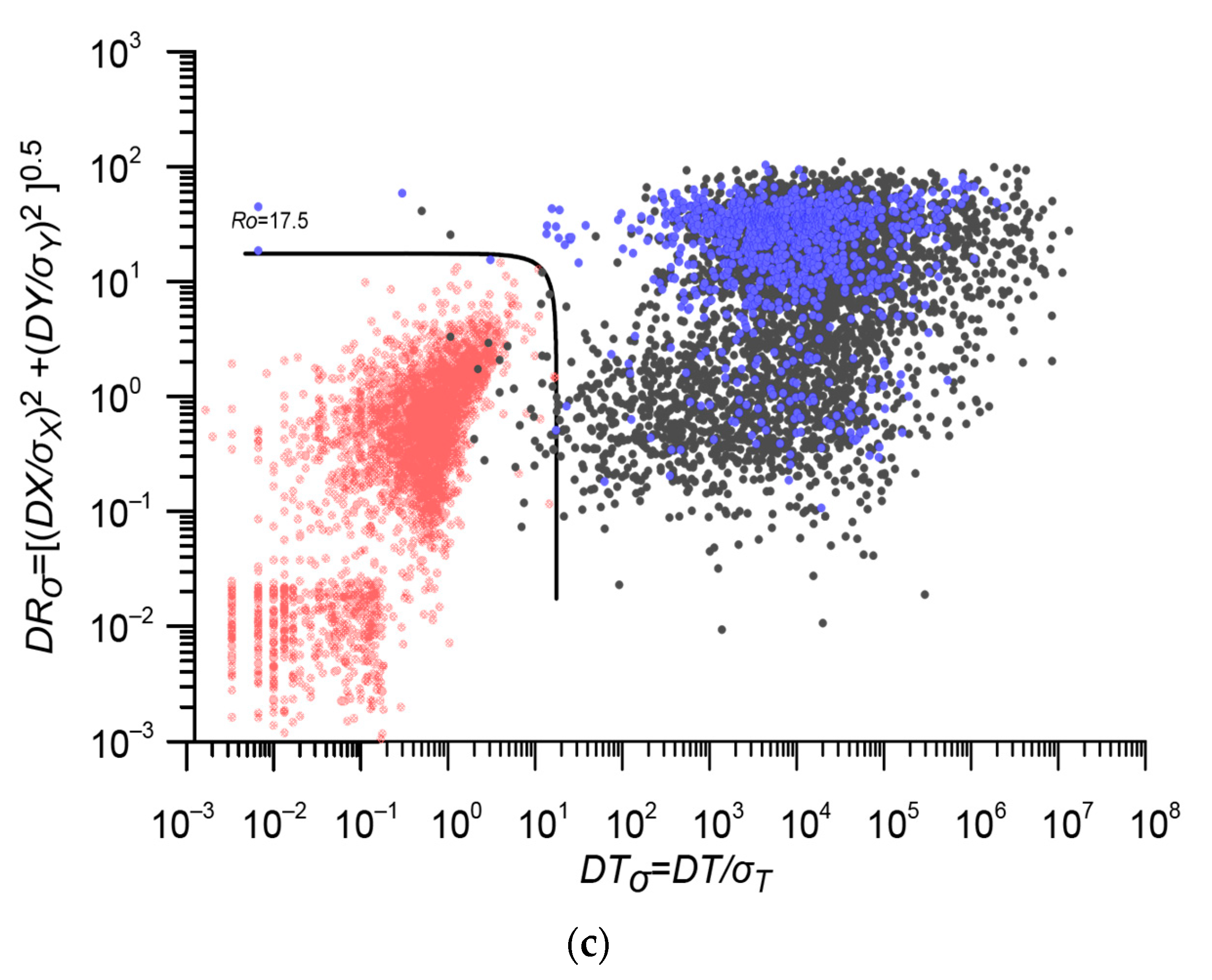
| 3 | ISC 16,937 events | RUS 4891 events | 0.05; 28.3; 24.7 | 17.5 | 0.9% | 3906 | ISC_RUS 17,922 events |
| 4 | Morozov 4 events | ISC_RUS 17,922 events | 4 | N_ARCTIC0 17,922 |


3.2. Magnitude Unification in the Integrated Earthquake Catalog
3.2.1. Svalbard
| Agency | Type of Magnitude | Priority | Number of Events | Magnitude in the Integrated Catalog | Correlation | Figure | Mmin— Mmax. Initial Magnitude Scale | Note |
|---|---|---|---|---|---|---|---|---|
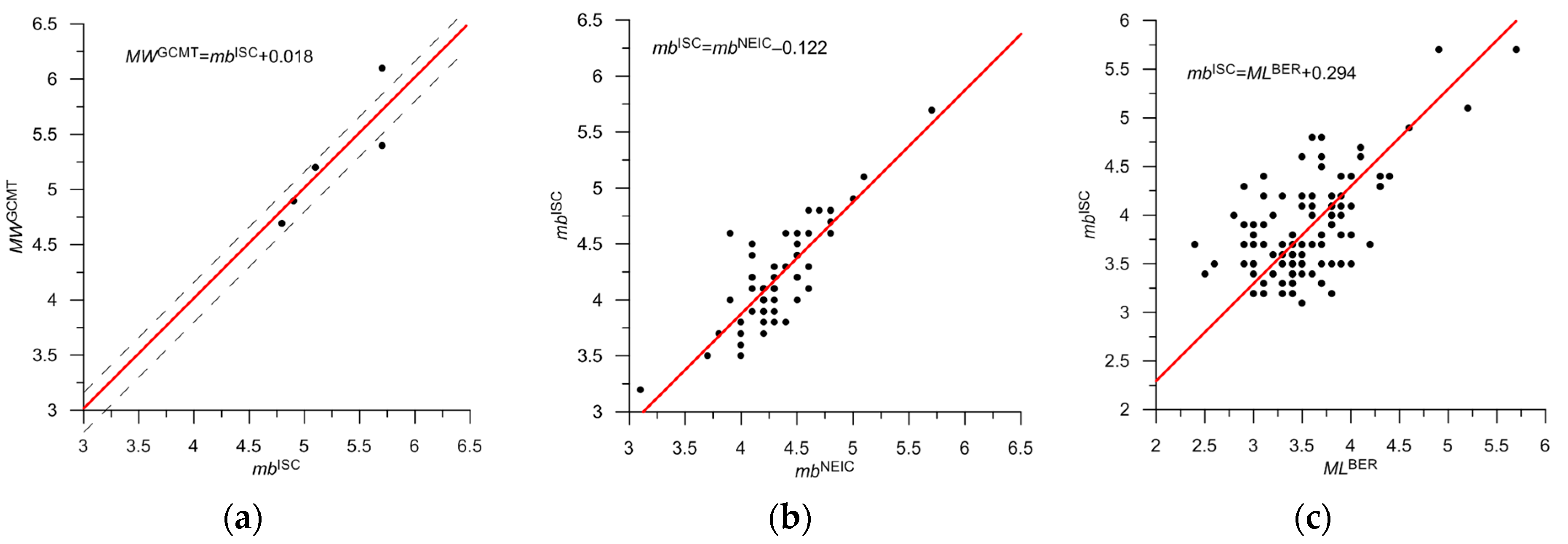
| GCMT | MW | 1 | 6 | M = MWGCMT | 4.7–6.1 | |||
| ISC | mb | 2 | 130 | M = mbISC | 0.78 | 11a | 3.1–5.6 | |
| NEIC, NEIS | mb | 2 | 17 | M=mbNEIC–0.1 | 0.75 | 11b | 3.3–4.9 | |
| BER | ML | 3 | 5927 | M = MLBER + 0.3 | 0.39 | 11c | 0.3–3.9 | |
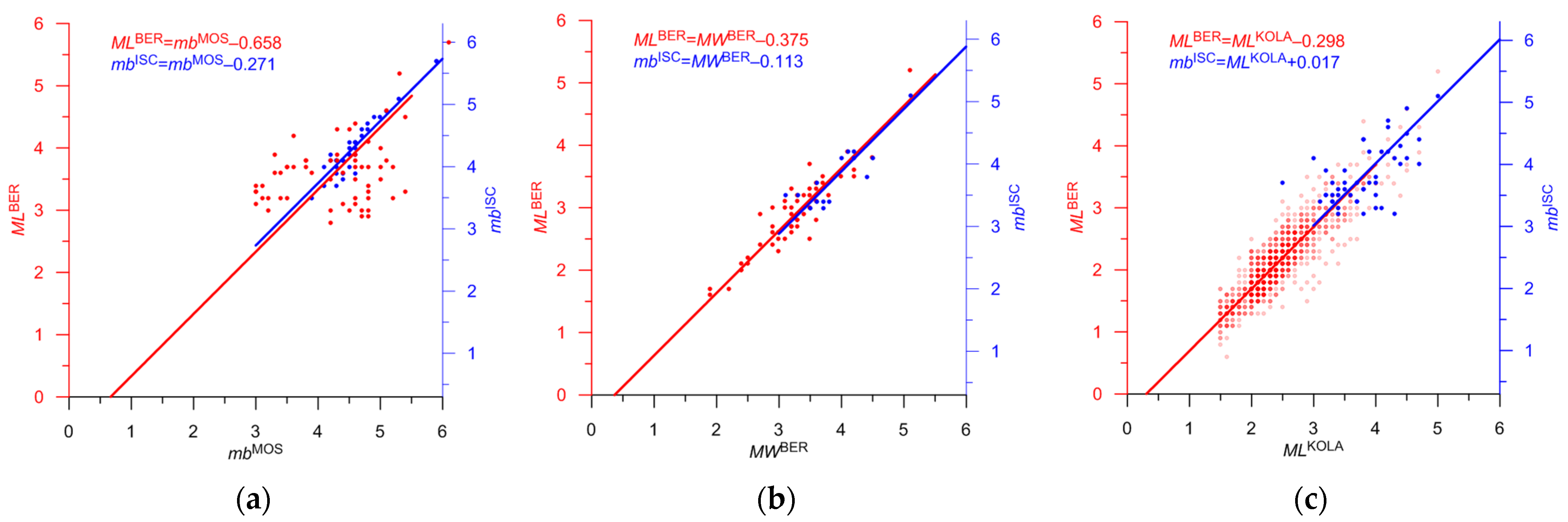
| KOLA | ML | 4 | 330 | M = MLKOLA | 0.79 | 12c | 1.4–3.4 | |
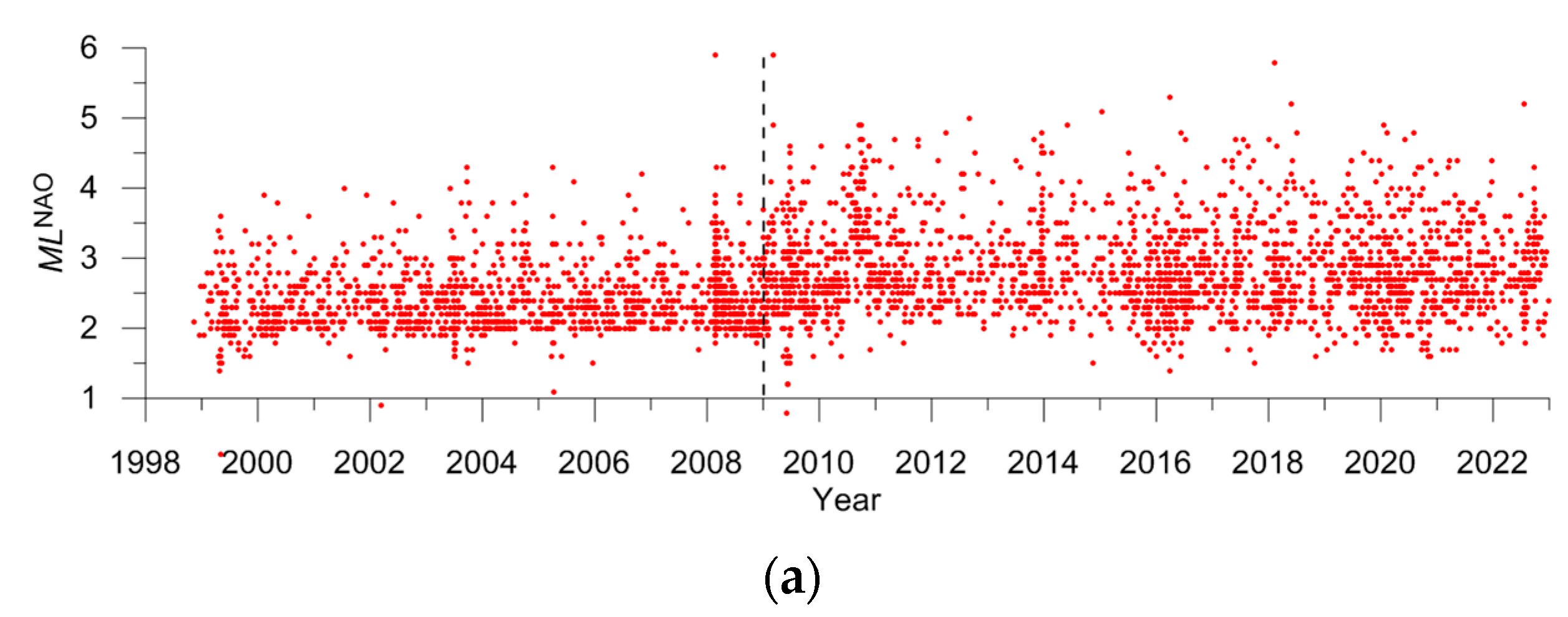
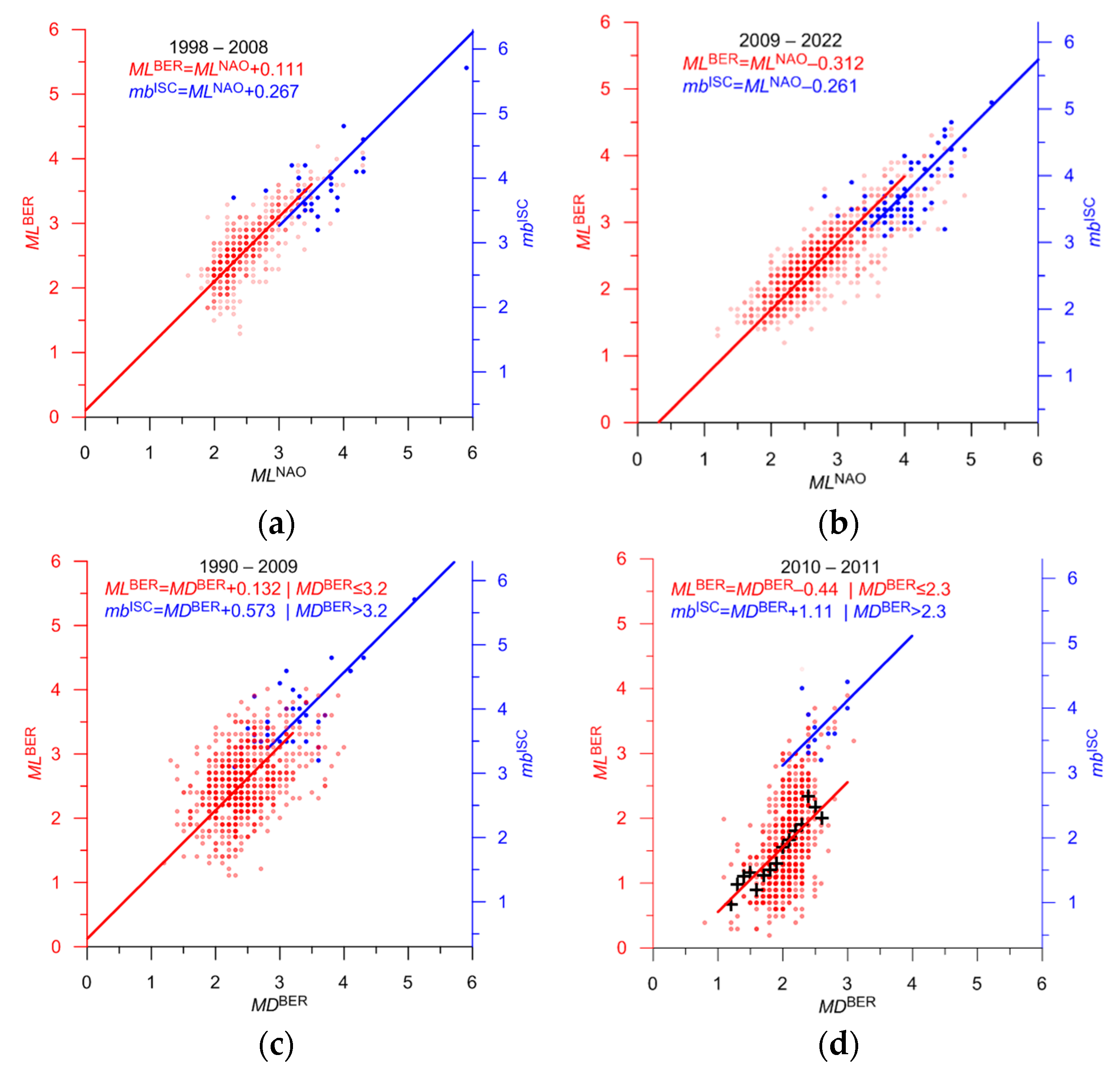
| NAO | ML | 4 | 250 | M = MLNAO + 0.4 | 0.65 | 13a | 0.9–3.2 | 1998–2008 |
| NAO | ML | 4 | 47 | M = MLNAO | 0.53 | 13b | 1.2–3.5 | 2009–2022 |
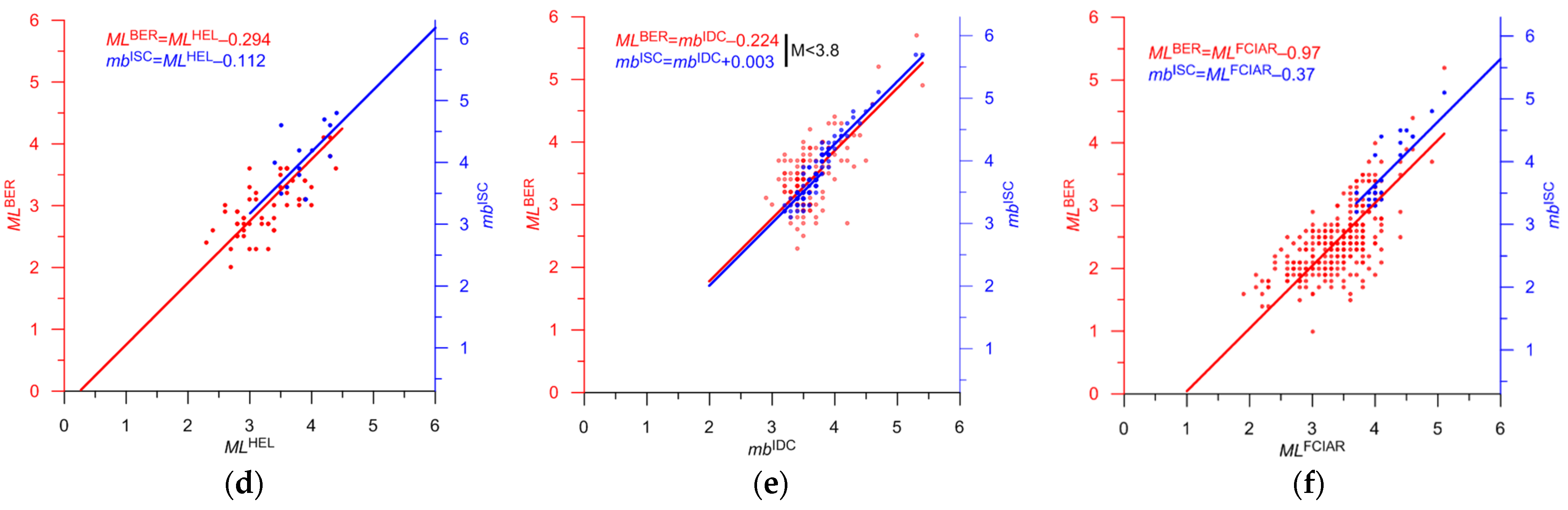
| FCIAR | ML | 4 | 46 | M = MLFCIAR–0.7 | 0.47 | 12f | 1.8–3.8 | |
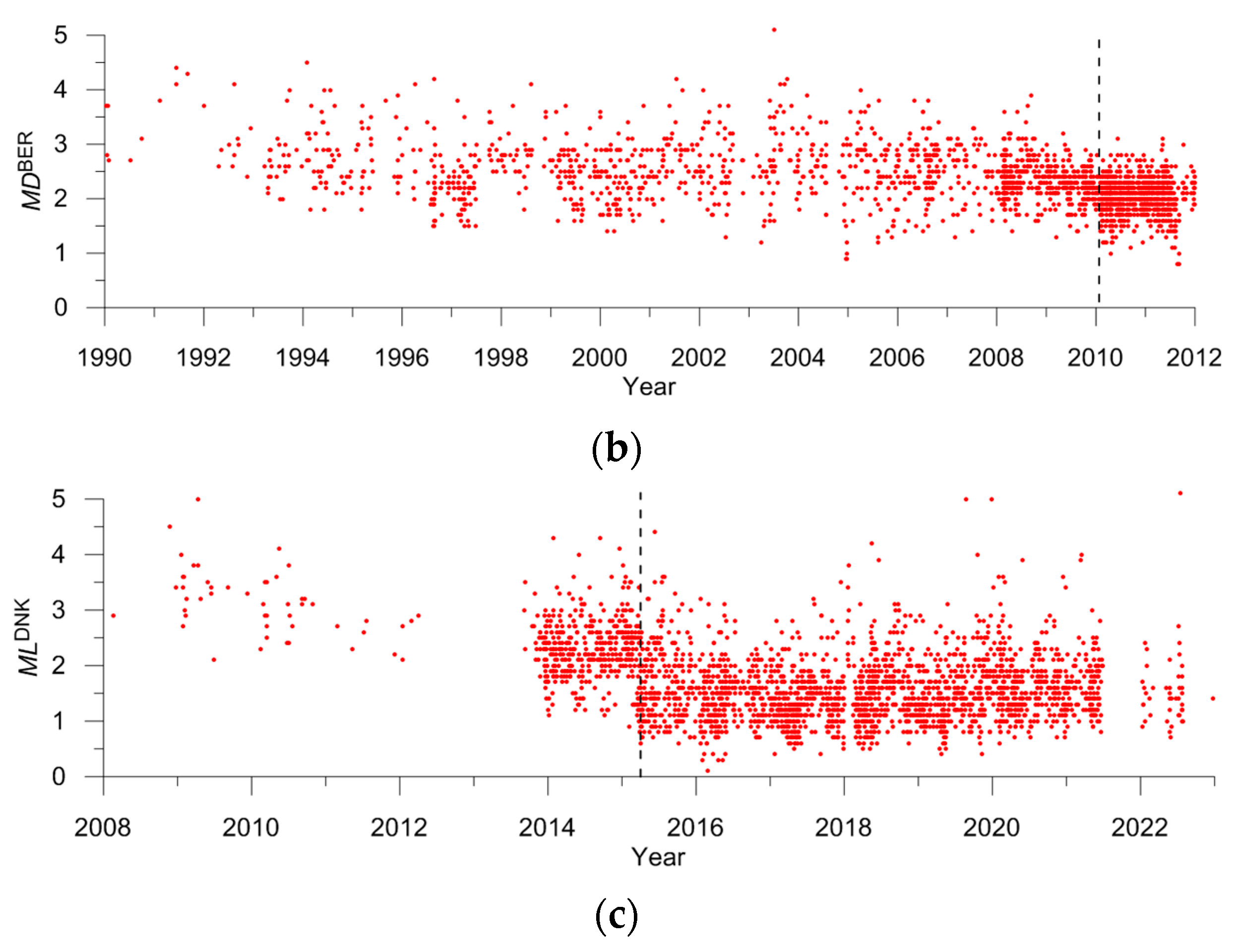
| BER | MD | 4 | 92 | M = MDBER + 0.4 | 0.43 | 13c | 0.9–3.2 | 1990–2009 |
| BER | MD | 5 | 34 | M = MDBER–0.1 | 0.25 | 13d | 0.8–2.3 | 2010–2011 unreliable, Non-linear relation |
| MOS | mb | 4 | 2 | M = mbMOS–0.3 | 0.89 | 12a | 4.9–5.8 | |
| BER | Mw | 4 | 7 | M = MwBER–0.1 | 0.85 | 12b | 3.1–3.9 | |
| HEL | ML | 4 | 4 | M = MLHEL | 0.53 | 12d | 2.3–3.2 | |
| IDC | mb | 4 | 1 | M = mbIDC | 0.78 | 12e | 3.5 | |
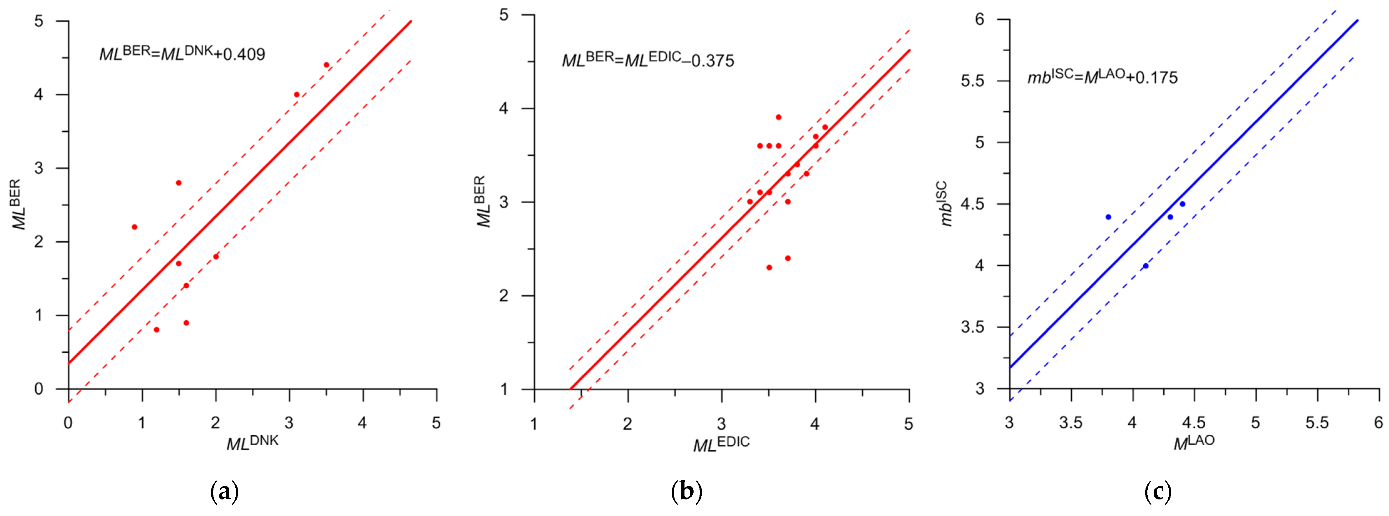
| DNK | ML | 5 | 3 | M = MLDNK + 0.7 | 0.66 | 14a | 1.8–2.0 | Poorly determined |
| EDIC | ML | 5 | 7 | M = MLEIDC–0.1 | 0.20 | 14b | 2.8–4.0 | Poorly determined |
| LAO | M | 5 | 2 | M = MLAO + 0.2 | 0.07 | 14c | 3.4–3.8 | Poorly determined |
| NAO | mb | 5 | 1 | M = mbNAO | 4 | Not Determined | ||
| HEL | MD | 5 | 5 | M = MDHEL | 3.2–4.0 | Not Determined | ||
| BER | mb(Pn) | 5 | 4 | M = mb(Pn)BER | 2.5–2.8 | Not Determined | ||
| WAR | M | 5 | 5 | M = MWAR | 2.1–3.0 | Not Determined | ||
| NUR | M | 5 | 1 | M = MNUR | 3.9 | Not Determined | ||
| Total | 6921 |
3.2.2. Knipovich and Gakkel Ridges
| Agency | Type of Magnitude | Priority | Number of Events | Magnitude in the Integrated Catalog | Correlation | Figure | Mmin— Mmax. Initial Magnitude Scale | Note |
|---|---|---|---|---|---|---|---|---|
| GCMT | MW | 1 | 112 | M = MWGCMT | – | 4.6–6.7 | ||
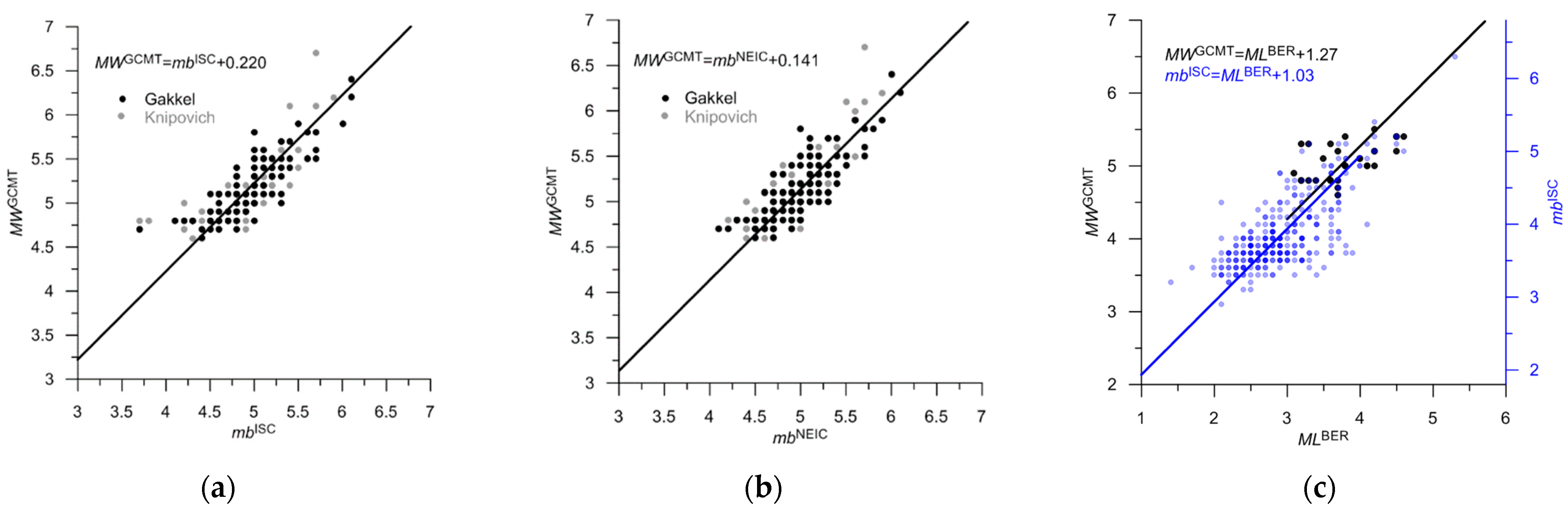
| ISC | mb | 2 | 805 | M = mbISC + 0.2 | 0.67 | 15a | 2.9–6.3 | Gakkel and Knipovich |
| NEIC, NEIS | mb | 2 | 80 | M = mbNEIC + 0.1 | 0.66 | 15b | 3.3–4.9 | Gakkel and Knipovich |
| BER | ML | 3 | 2974 | M = MLBER + 1.2 | 0.54 | 15c | 0.3–3.7 | Knipovich |
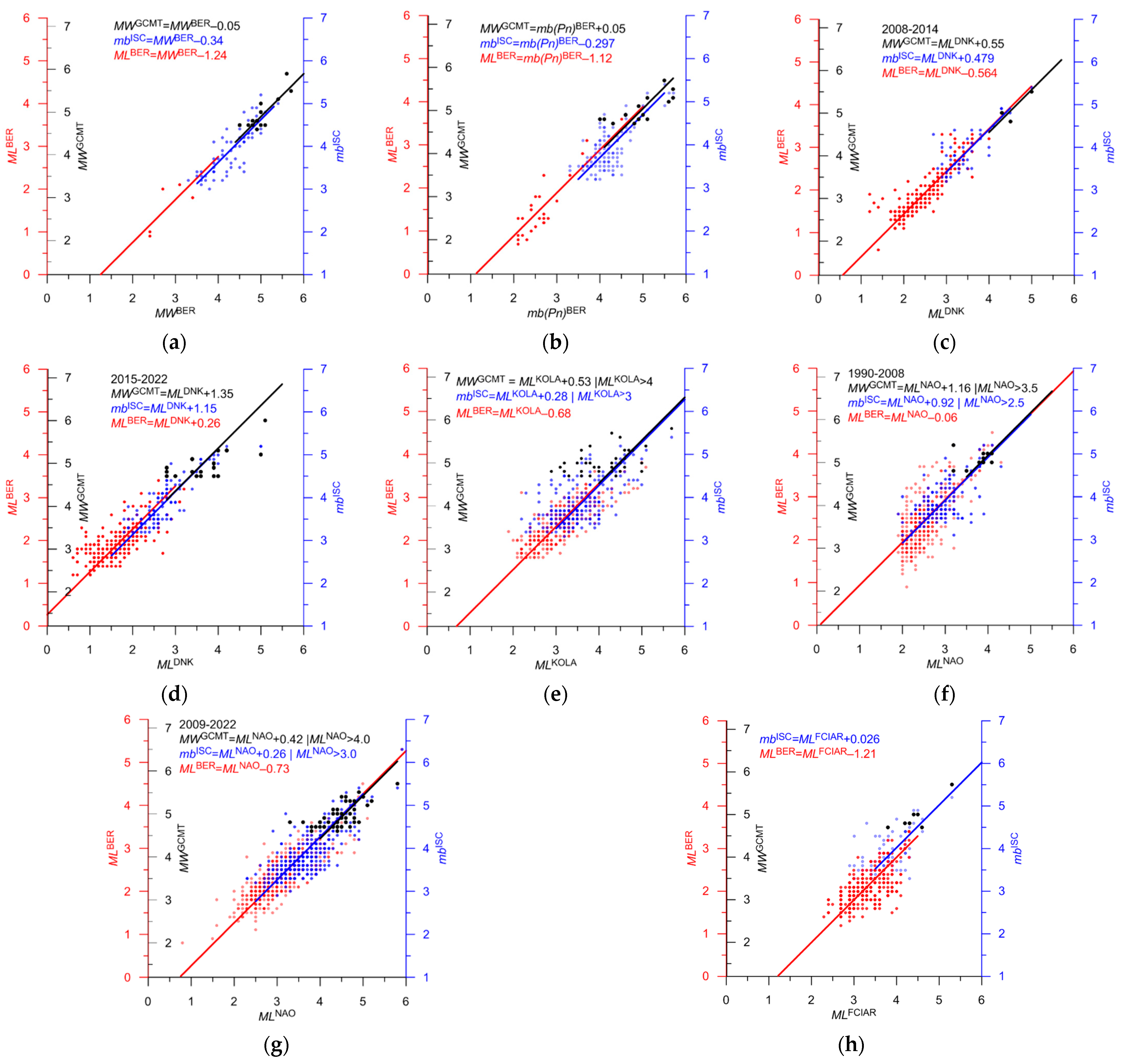
| BER | Mw | 4 | 1892 | M = MwBER − 0.1 | 0.72 | 16a | 1.3–5.0 | Gakkel and Knipovich |
| BER | mb(Pn) | 4 | 1521 | M = mb(Pn)BER − 0.1 | 0.82 | 16b | 1.7–4.6 | Gakkel and Knipovich |
| DNK | ML | 4 | 83 | M = MLDNK + 0.6 | 0.79 | 16c | 0.9–3.1 | 2008–2015.2 Knipovich |
| DNK | ML | 4 | 753 | M = MLDNK + 1.3 | 0.57 | 16d | 0.1–3.1 | 2015.3–2022 Knipovich |
| KOLA | ML | 4 | 82 | M = MLKOLA + 0.5 | 0.65 | 16e | 1.3–3.4 | Knipovich |
| NAO | ML | 4 | 265 | M = MLNAO + 1.1 | 0.53 | 16f | 0.2–3.4 | 1990–2008 Gakkel and Knipovich |
| NAO | ML | 4 | 32 | M = MLNAO + 0.4 | 0.69 | 16g | 1.7–4.2 | 2009–2022 Gakkel and Knipovich |
| FCIAR | ML | 4 | 102 | M = MLFCIAR | 0.42 | 16h | 2.3–4.1 | Knipovich |
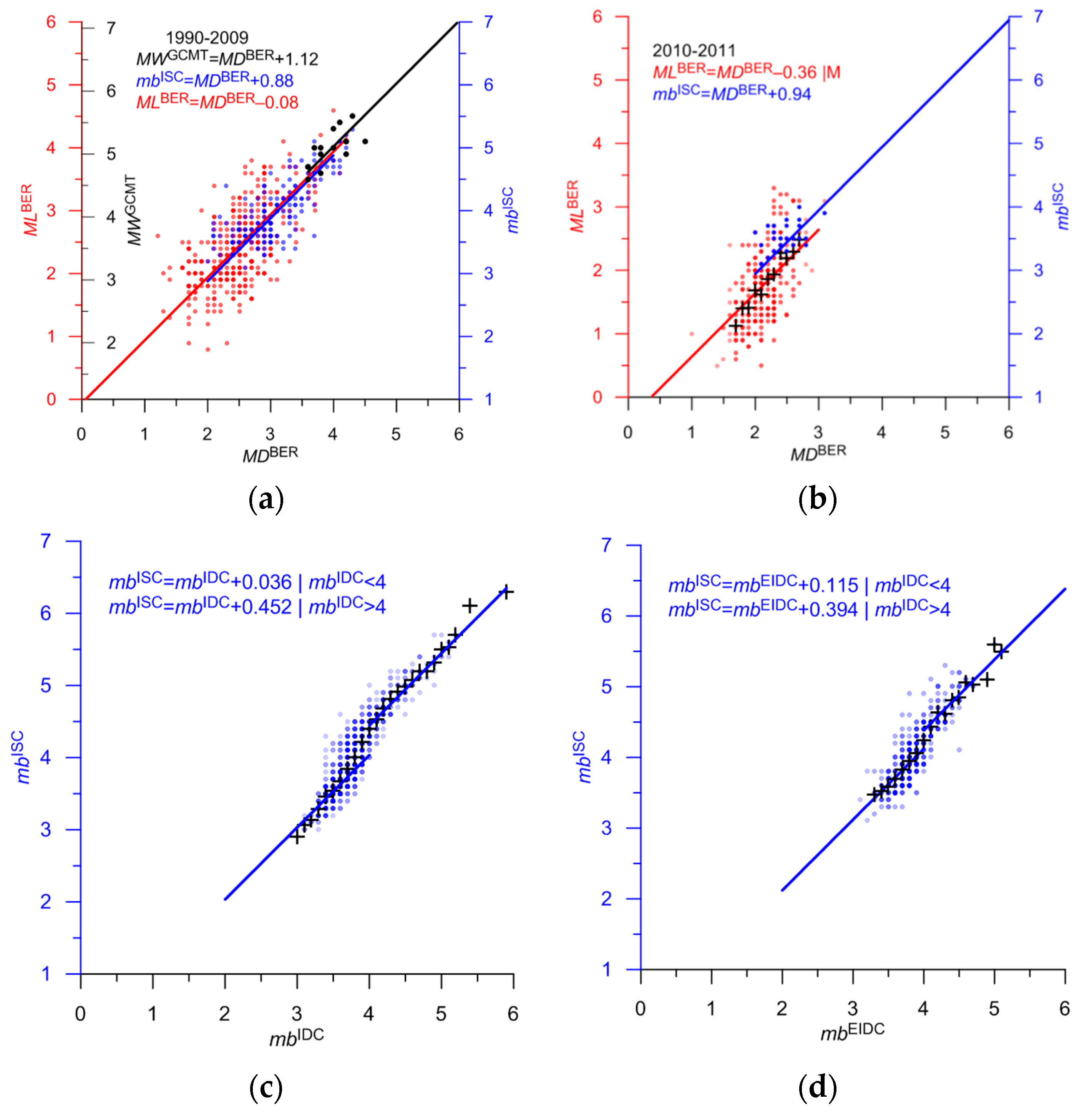
| BER | MD | 5 | 96 | M = MDBER + 1.1 | 0.62 | 17a | 1.5–4.4 | 1990–2009 Knipovich |
| BER | MD | 5 | 20 | M = MDBER + 0.8|MD < 2.7 | 0.23 | 17b | 1.5–2.5 | 2010–2011 Knipovich, unreliable |
| IDC | mb | 4 | 21 | M = mbIDC + 0.2 | 0.85 | 17c | 3.0–3.6 | Gakkel and Knipovich |
| EIDC | mb | 4 | 11 | M = mbEIDC + 0.3 | 0.76 | 17d | 2.9–3.7 | Gakkel and Knipovich |
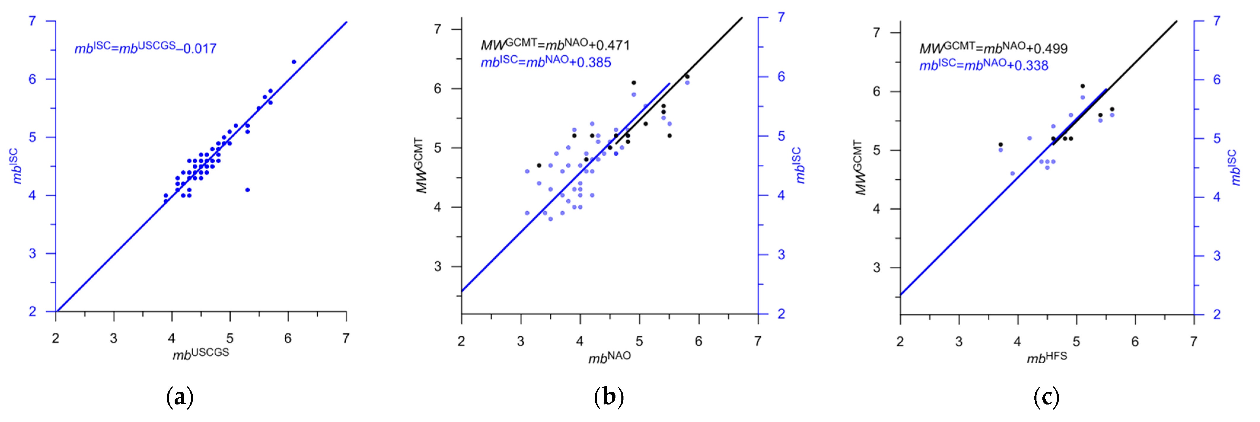
| USCGS | mb | 4 | 4 | M = mbUSCGS + 0.2 | 0.83 | 18a | 4.2–4.6 | Gakkel and Knipovich |
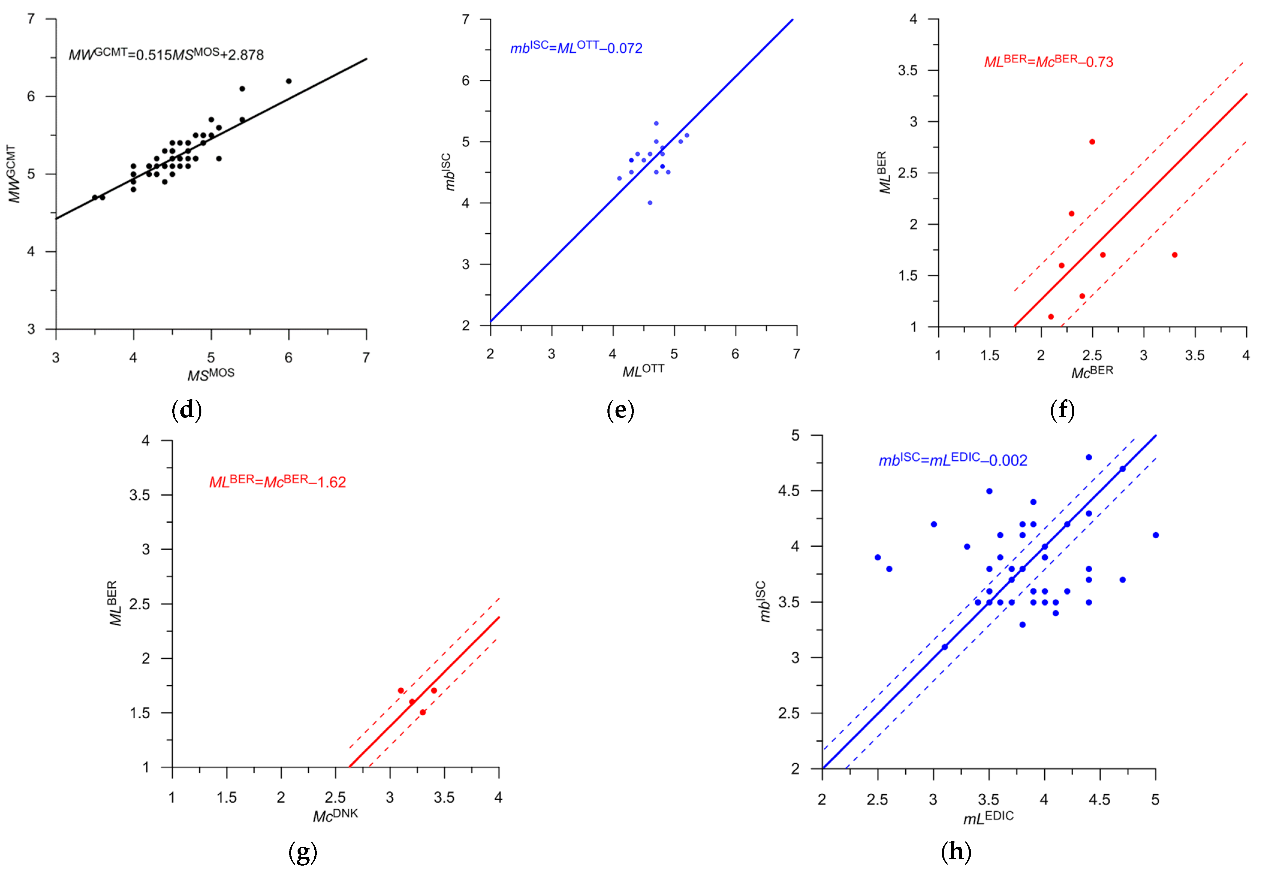
| MOS | MS | 4 | 1 | M = 0.515MSISC + 2.88 | 0.71 | 18d | 4.7 | Gakkel and Knipovich |
| NAO | mb | 4 | 3 | M = mbNAO + 0.5 | 0.62 | 18b | 3.6–4.1 | Knipovich |
| HFS | mb | 4 | 1 | M = mbNAO + 0.5 | 0.50 | 18c | 3.9 | Knipovich |
| OTT | ML | 4 | 27 | M = MLOTT + 0.1 | 0.23 | 18e | 3.2–5.0 | Gakkel and Knipovich |
| EIDC | ML | 5 | 7 | M = MLEIDC + 0.2 | 0.05 | 18h | 3.4–4.2 | Poorly determined |
| BER | Mc | 5 | 3 | M = McBER + 0.4 | 0.03 | 18f | 1.7–3.2 | Poorly determined |
| DNK | Mc | 5 | 6 | M = McBER − 0.5 | 0 | 18g | 2.1–3.7 | Poorly determined |
| CGS | M | 5 | 5 | M = MCGS | 4.2–4.7 | Not Determined | ||
| DNK | MD | 5 | 1 | M = MDBER | 2.4 | Not Determined | ||
| PAL | M | 5 | 2 | M = MPAL | 4.3 | Not Determined | ||
| STU | M | 5 | 1 | M = MSTU | 5.2 | Not Determined | ||
| OTT | Mn | 5 | 1 | M = MnOTT | 3.1 | Not Determined | ||
| WAR | M | 5 | 1 | M = MWAR | 2.6 | Not Determined | ||
| Total | 8912 |


3.3. Statistics of the Integrated Catalog for Three Sub-Regions
| Time Period, Catalog * | N Total | N from ISC | N from GS RAS, Morozov | Mc | N, M ≥ Mc | Mmax |
|---|---|---|---|---|---|---|
| 1962–2022 | ||||||
| N_Arctic | 17,922 | 16,933 (94.2%) | 989 (5.8%) | - | 6.7 | |
| Svalbard | 6921 | 6617 (95.6%) | 304 (4.4%) | - | 6.1 | |
| Knipovich Ridge | 8912 | 8794 (98.7%) | 118 (1.3%) | - | 6.7 | |
| Gakkel Ridge | 2089 | 1522 (72.9%) | 567 (27.1%) | - | 6.5 | |
| 1962–1994 | ||||||
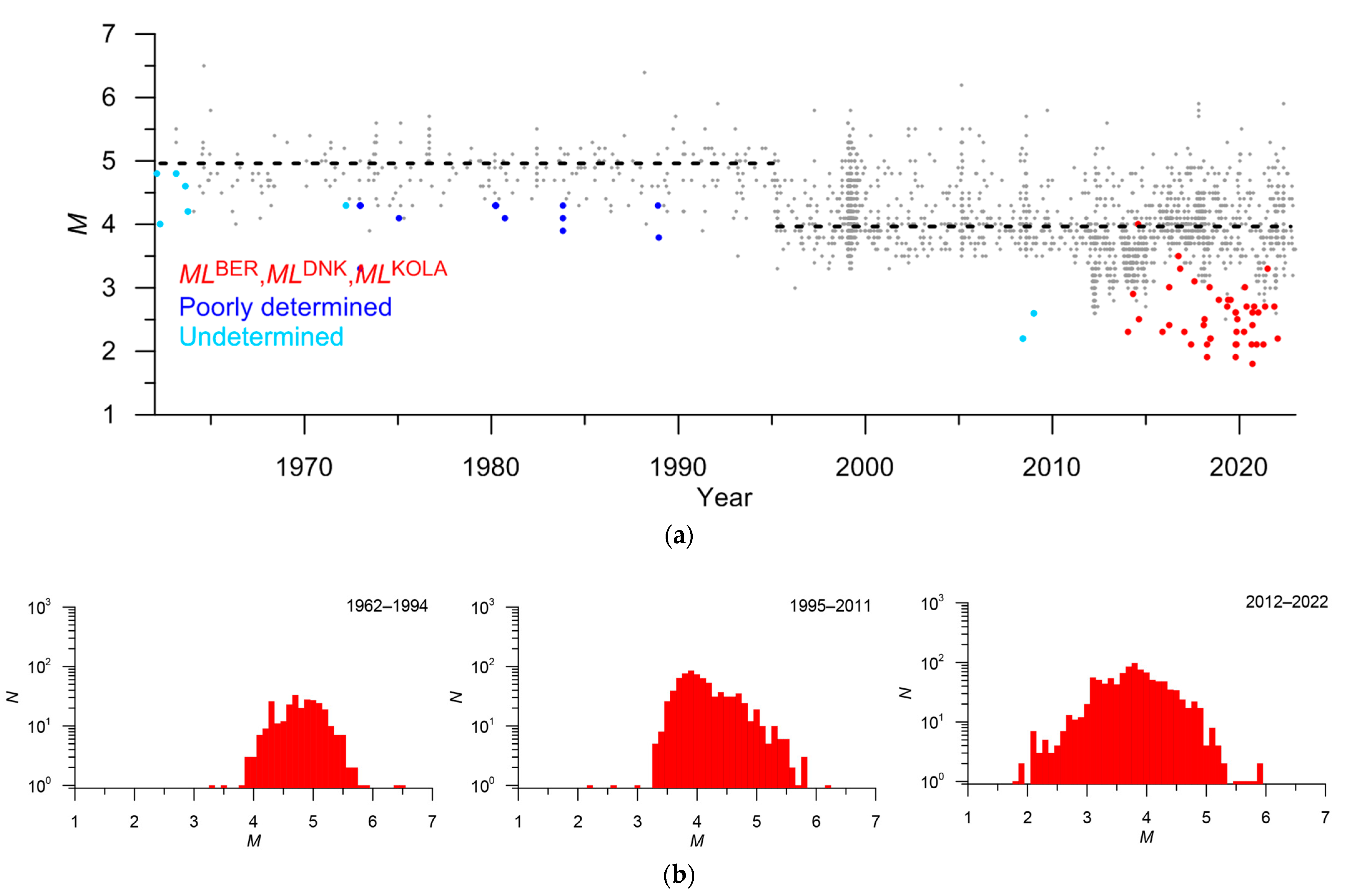
| N_Arctic | 703 | 683 (97.2%) | 20 (2.8%) | 5.0 | 181 | 6.7 |
| Svalbard | 94 | 94 (100%) | 0 (0%) | 4.5 | 20 | 5.6 |
| Knipovich Ridge | 329 | 329 (100%) | 0 (0%) | 4.7 | 166 | 6.7 |
| Gakkel Ridge | 280 | 260 (92.9%) | 20 (7.1%) | 5.0 | 102 | 6.5 |
| 1995–2011 | ||||||
| N_Arctic | 4377 | 4261 (97.3%) | 116 (2.7%) | 4.0 | 762 | 6.5 |
| Svalbard | 2209 | 2103 (95.2%) | 105 (4.8%) | 2.8 | 696 | 6.1 |
| Knipovich Ridge | 1408 | 1405 (99.8%) | 3 (0.2%) | 4.0 | 275 | 6.5 |
| Gakkel Ridge | 760 | 752 (98.9%) | 8 (1.1%) | 4.0 | 454 | 6.2 |
| 2012–2022 | ||||||
| N_Arctic | 12,842 | 11,989 (95.4%) | 853 (6.6%) | 4.0 | 657 | 6.0 |
| Svalbard | 4618 | 4419 (95.7%) | 199 (4.3%) | 1.7 | 2351 | 5.3 |
| Knipovich Ridge | 7175 | 7060 (98.4%) | 115 (1.6%) | 2.8 | 3447 | 6.0 |
| Gakkel Ridge | 1049 | 510 (48.6%) | 539 (51.4%) | 4.0* | 388 | 5.9 |


4. Conclusions
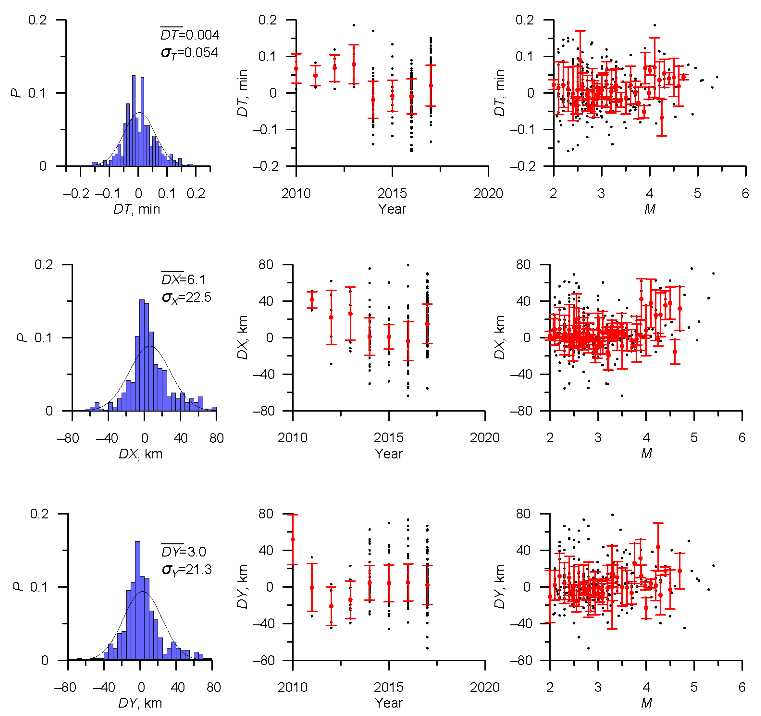
- The earthquake catalogs of the studied region (the Gakkel and Knipovich mid-ocean ridges plus the Svalbard Archipelago) are a mixture of data from a large number of agencies. Moreover, the catalogs significantly vary over time. As a result, heavy tails appear in the DT, DX, and DY distributions. Therefore, determining the threshold value of the metric using the methodology applied in [27,28] leads to an increased probability of missing duplicates. For this reason, in this study, we decided not to use a multivariate normal distribution model. Instead, the actual distribution of the metric for the nearest events from two combined catalogs was used. As a result, the estimated number of errors in the integrated catalog does not exceed 1%;
- The integrated catalog contains 17,922 events; 16,933 are from the ISC and 989 events are from Russian catalogs. The latter were not presented in the ISC, while the information regarding 578 events from Russian catalogs was used as a part of the ISC data. In the Gakkel Ridge, Russian data accounts for more than a quarter of events, and more than half after 2012. In the sub-regions of Svalbard and Knipovich, the addition of ISC data with Russian catalogs is insignificant. However, an important aspect here is the unification of magnitude;
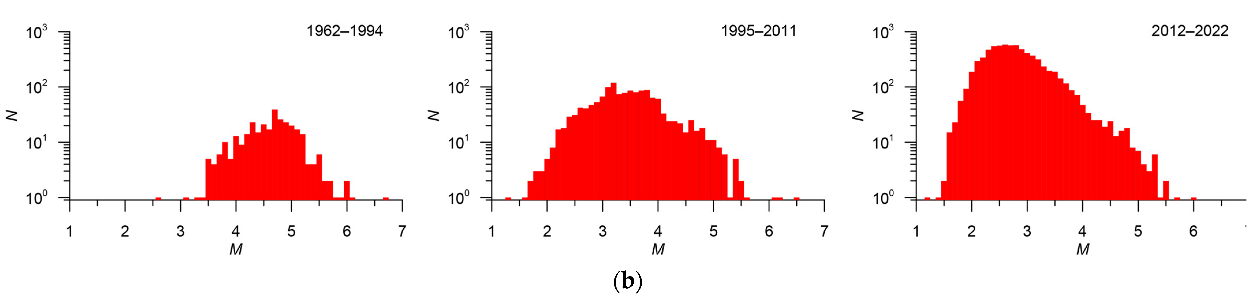
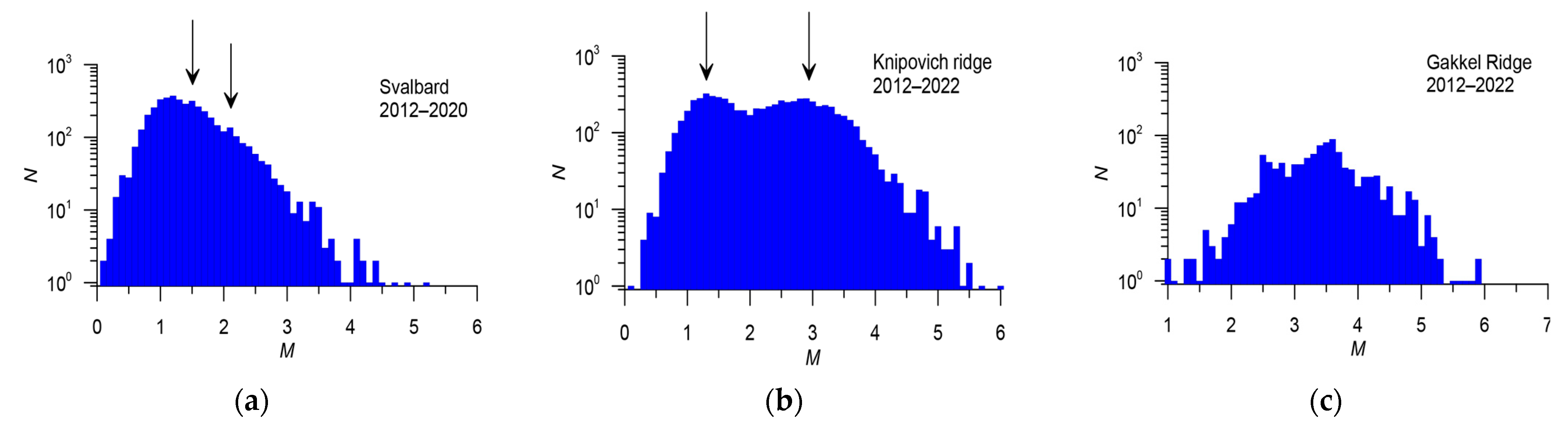
- The ratios between local magnitudes ML with the reference magnitude MWGCMT and mbISC significantly differ in Svalbard and mid-ocean ridges. In Svalbard, the difference between the local and moment magnitudes is about 0.3 (Table 3). In the Knipovich and Gakkel ridges, the estimates of local magnitudes are significantly underestimated compared to the moment magnitude, with a difference exceeding 1.0 (Table 4 and Table 5). Figure 25 shows the frequency-magnitude distributions constructed using original magnitudes. In Svalbard, noticeable discontinuities in the distribution are observed (Figure 25a). This can significantly affect the estimates of the b-value (the slope of the magnitude-frequency plot), which is an important parameter in seismic hazard assessment. The distribution in the Knipovich Ridge (Figure 25b) has a bimodal character, which contradicts the Gutenberg-Richter law. This is an independent confirmation of the inconsistency of magnitude estimates ML and MWGCMT, mbISC. In the Gakkel Ridge (Figure 25c), the distribution weakly follows the Gutenberg-Richter law. After the proposed magnitude conversion, the magnitude-frequency plots acquired a common form (Figure 21b, Figure 22b and Figure 23b);
- 4.
- When creating the unified magnitude scale, ratios were used with three types of magnitude, MWGCMT, mbISC, and MLBER, which are well represented in the studied region. The shift-type ratios turned out to be very similar for most magnitudes of different types determined by various agencies. This approach allows for a significant expansion of the interval for converting magnitudes to proxy-MW, increases statistics, and thus increases the reliability of the conversion. The MWGCMT magnitude is only determined for strong earthquakes with M > 5.0. The use of correlations with mbISC and MLBER allows for an extension of the interval to M of the order of 1. Strictly mathematically, this is not proof of the linearity of ratios between different magnitudes, but it is a weighty argument in favor of such an assumption;
- 5.
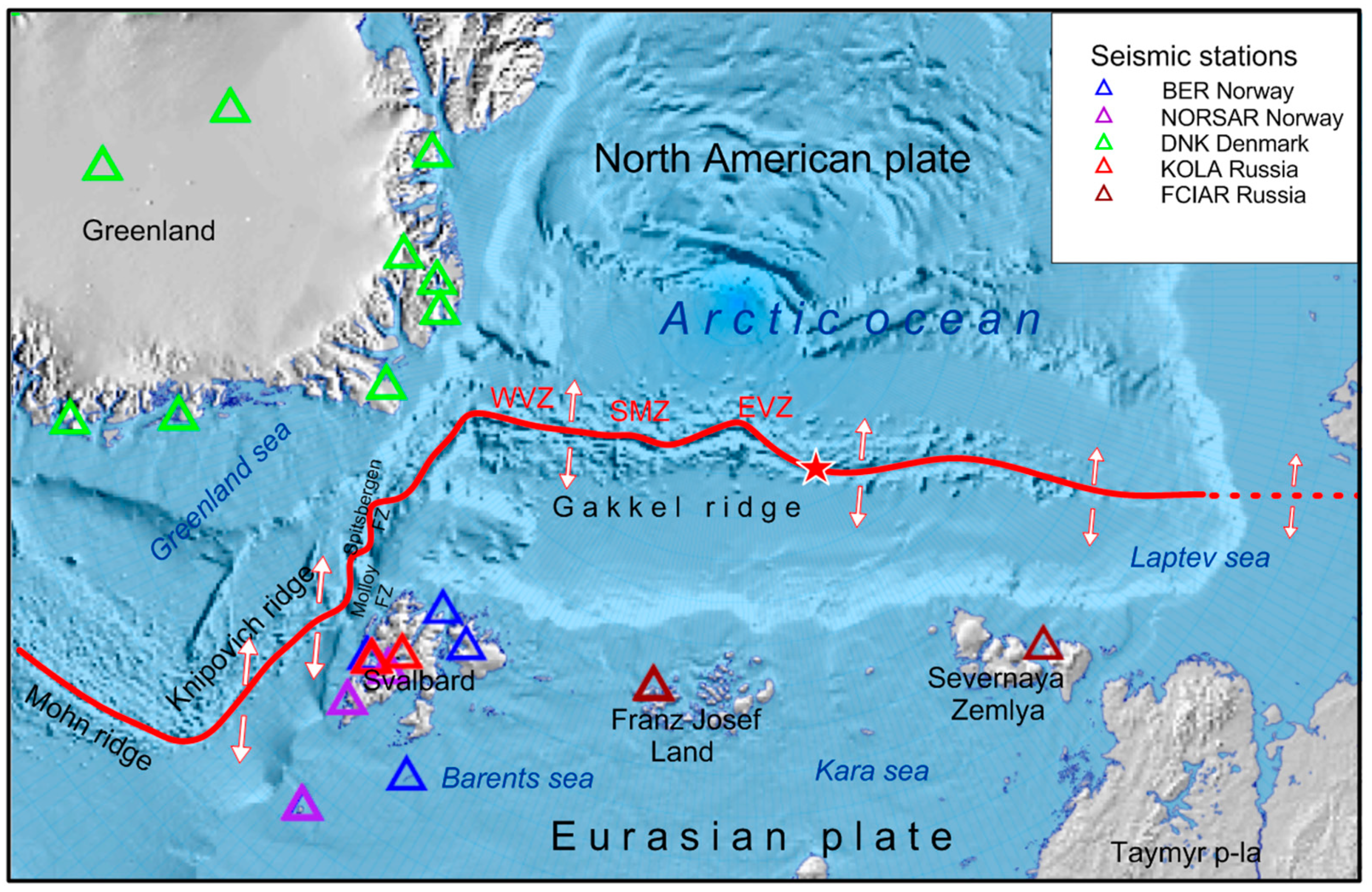
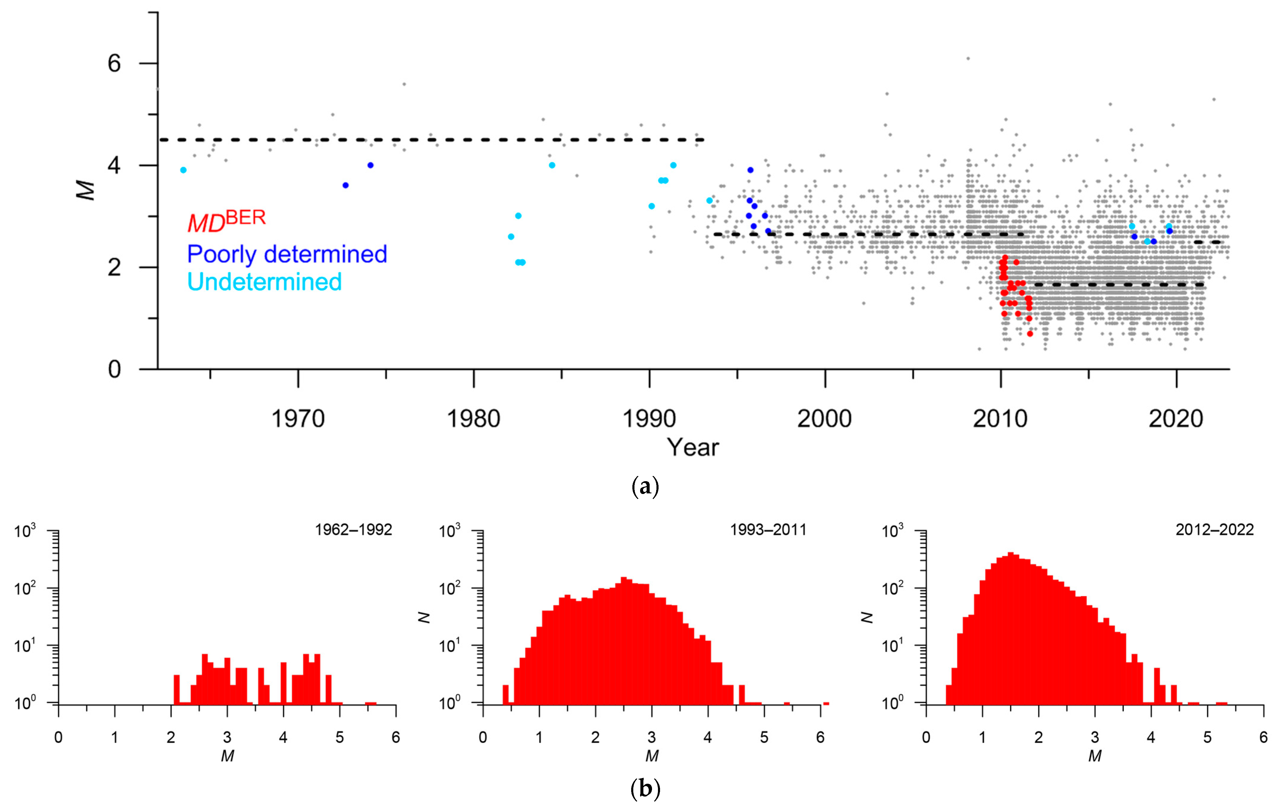
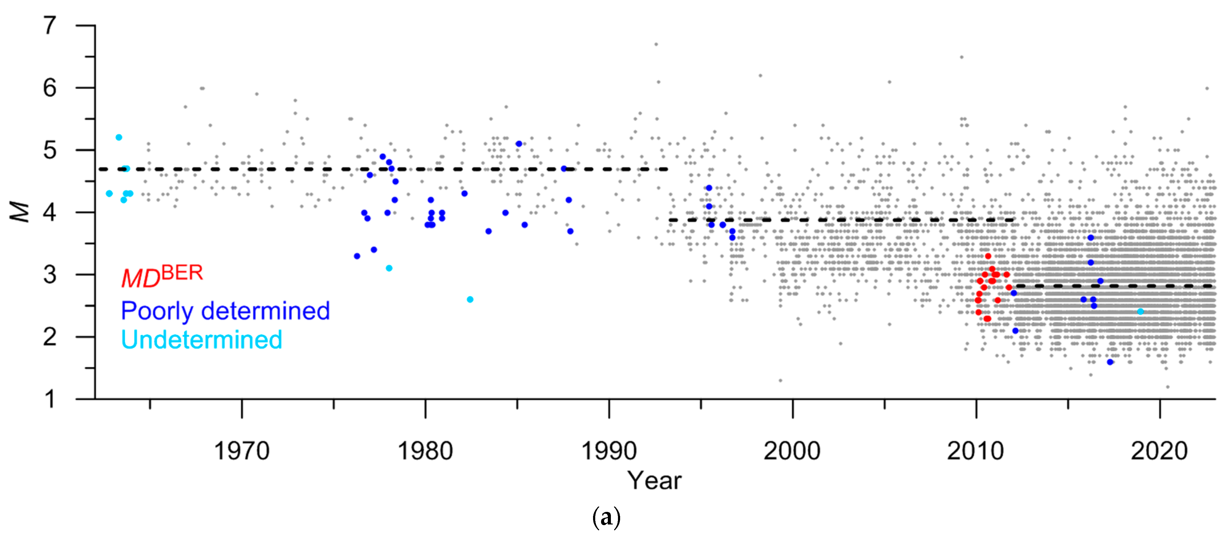
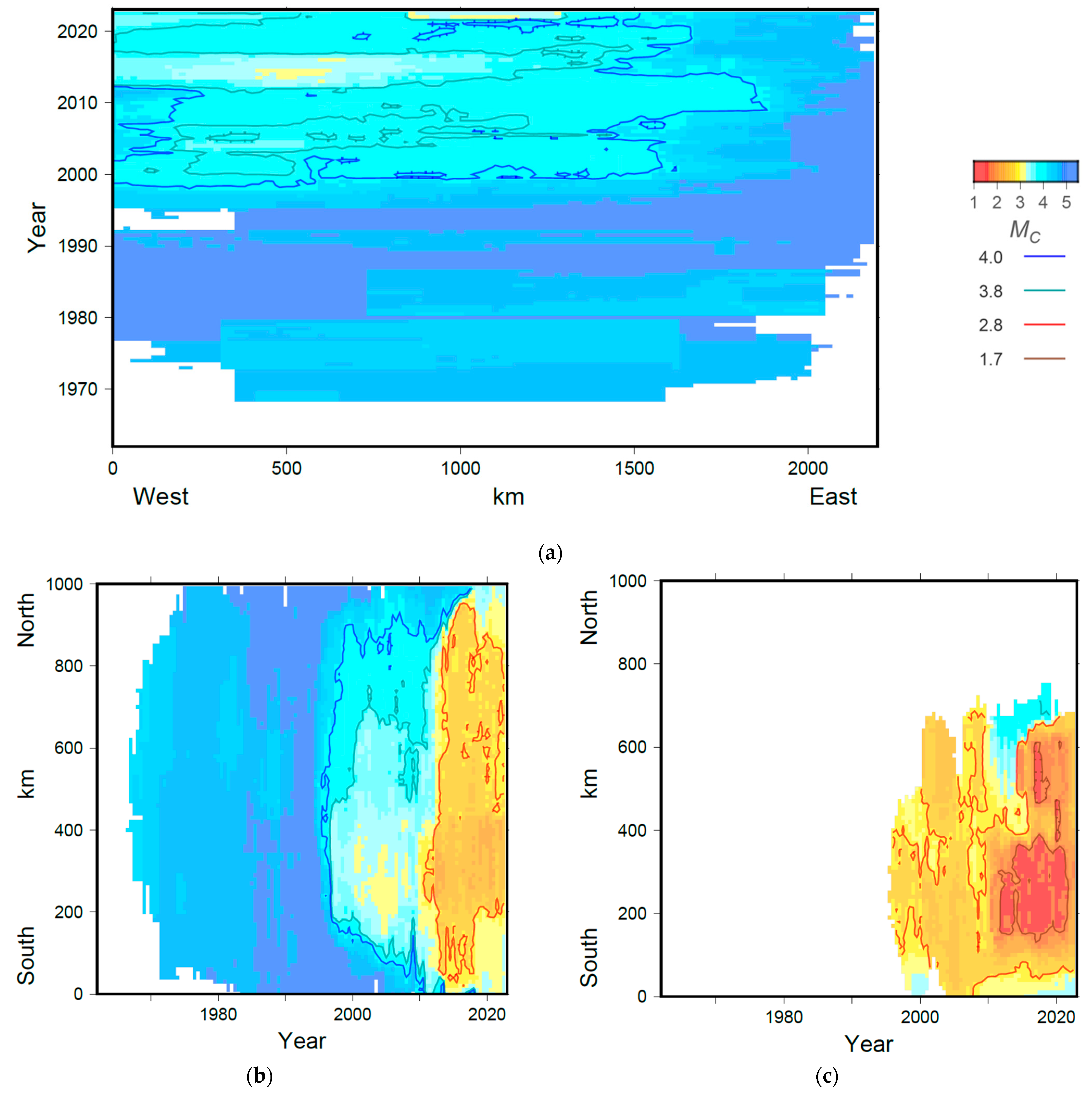
- The level of registration significantly varies over time and differs in sub-regions. The best registration level is on Svalbard (Mc = 1.7 after 2012), where there are many seismic stations of the BER, NORSAR, and KOLA networks. A good registration level is apparent in the Knipovich Ridge (Mc = 2.8 after 2012), which is provided by Norwegian and Russian stations on Svalbard and Danish DNK stations in Greenland. The worst registration level is in the Gakkel Ridge (Mc = 4.0), which is not surprising. The nearest seismic stations of FCIAR are located on the archipelagos of Severnaya Zemlya and Franz Josef Land, approximately 600 km from the seismic zone. The distance from Svalbard stations to the Gakkel Ridge is approximately the same;
- 6.
- The integrated earthquake catalog created and reported in this paper is intended for a wide range of researchers involved in both the study of the seismic regime of the Arctic and, in general, seismic hazard assessment [35,36,37,38,39,40,41,42,43,44,45,46]. Presented here, the integrated earthquake catalog, along with the author’s Arctic catalogs [27,28], provides an important contribution to the development of an Arctic Big Data system. Its creation is one of the important requirements for starting a full-scale system analysis of geophysical dynamics in the Arctic;
- 7.
- Figure S6 (see Supplementary) presents all three created integrated earthquake catalogs for the Arctic zone of the Russian Federation. The integrated catalog of Arctic regions I, II, and III contains 45,793 events. In the Svalbard region, 12 duplicates were identified and removed. We believe that the magnitude scale is homogeneous, because all magnitudes were converted to proxi-Mw. The catalog is available to the public at: http://www.wdcb.ru/arctic_antarctic/arctic_seism.html (accessed on 1 August 2023).
Supplementary Materials
Author Contributions
Funding
Institutional Review Board Statement
Informed Consent Statement
Data Availability Statement
Acknowledgments
Conflicts of Interest
Abbreviations
| BCIS | Bureau Central International de Sismologie, France |
| BER | University of Bergen, Norway |
| CSEM | Centre Sismologique Euro-Méditerranéen (CSEM/EMSC), France |
| DNK | Geological Survey of Denmark and Greenland, Denmark |
| EIDC | Experimental (GSETT3) International Data Center, USA |
| FCIAR | Federal Center for Integrated Arctic Research, Russia |
| GFZ | Helmholtz Centre Potsdam GFZ German Research Centre For Geosciences, Germany |
| HEL | Institute of Seismology, University of Helsinki, Finland |
| HFS | Hagfors Observatory, Sweden |
| IDC | International Data Centre, CTBTO, Austria |
| IEPN | Institute of Environmental Problems of the North, Russian Academy of Sciences, Russia |
| INMG | Instituto Português do Mar e da Atmosfera, I.P., Portugal |
| ISC | International Seismological Centre, United Kingdom |
| ISS | International Seismological Summary, United Kingdom |
| MOS | Geophysical Survey of Russian Academy of Sciences (GS RAS), Russia |
| KOLA | Kola Regional Seismic Centre, GS RAS, Russia |
| MSUGS | Michigan State University, Department of Geological Sciences, USA |
| NAO | Stiftelsen NORSAR, Norway |
| NEIC | National Earthquake Information Center, USA |
| OTT | Canadian Hazards Information Service, Natural Resources Canada |
| SYKES | Sykes Catalogue of earthquakes 1950 onwards |
| WAR | Institute of Geophysics, Polish Academy of Sciences, Poland |
| ZEMSU | USSR |
References
- Thiede, J.; The Shipboard Scientific Party. Polarstern Arctis XVII/2 Cruise Report: AMORE 2001 (Arctic Mid-Ocean Ridge Expedition). Alfred Wegener Inst. 2002, 421, 297. [Google Scholar]
- Schlindwein, V.; Muller, C.C.; Jokat, W. Microseismicity of the Ultraslow-Spreading Gakkel Ridge, Arctic Ocean: A Pilot Study. Geophys. J. Int. 2007, 169, 100–112. [Google Scholar] [CrossRef]
- Muller, C.; Jokat, W. Seismic evidence for volcanic activity discovered in Central Arctic. Eos Trans. AGU 2000, 81, 265–269. [Google Scholar] [CrossRef]
- Tolstoy, M.; Bohnenstiehl, D.R.; Edwards, M.H.; Kurras, G.J. Seismic character of volcanic activity at the ultraslow-spreading Gakkel Ridge. Geology 2001, 29, 1139–1142. [Google Scholar] [CrossRef]
- Cochran, J.R.; Kurras, G.J.; Edwards, M.H.; Coakley, B.J. The Gakkel Ridge: Bathymetry, gravity anomalies and crustal accretion at extremely slow spreading rates. J. Geophys. Res. Solid Earth 2003, 108, 2116–2137. [Google Scholar] [CrossRef]
- Cochran, J.R. Seamount volcanism along the Gakkel ridge, Arctic Ocean. Geophys. J. Int. 2008, 174, 1153–1173. [Google Scholar] [CrossRef]
- Michael, P.J.; Langmuir, C.H.; Dick, H.J.B.; Snow, J.E.; Goldsteink, S.L.; Graham, D.W.; Lehnertk, K.; Kurras, G.; Jokat, W.; Muhe, R.; et al. Magmatic and amagmatic seafloor generation at the ultraslow-spreading Gakkel ridge, Arctic Ocean. Nature 2003, 423, 956–961. [Google Scholar] [CrossRef] [PubMed]
- Dick, H.; Lin, J.; Schouten, H. An ultraslow-spreading class of ocean ridge. Nature 2003, 426, 405–412. [Google Scholar] [CrossRef] [PubMed]
- Zarayskaya, Y.A. Segmentation and seismicity of the ultraslow Knipovich and Gakkel mid-ocean ridges. Geotectonics 2017, 51, 163–175. [Google Scholar] [CrossRef]
- Dubinin, E.P.; Kokhan, A.V.; Sushchevskaya, N.M. Tectonics and magmatism of ultraslow spreading ridges. Geotectonics 2013, 47, 131–155. [Google Scholar] [CrossRef]
- Jokat, W.; Schmidt-Aursch, M. Geophysical characteristics of the ultraslow spreading Gakkel Ridge, Arctic Ocean. Geophys. J. Intern. 2007, 168, 983–998. [Google Scholar] [CrossRef]
- Kokhan, A.V.; Dubinin, E.P.; Grokholsky, A.L. Geodynamical peculiarities of structure-forming in Arctic and Polar Atlantic spreading ridges. Bull. Kamchatka Reg. Assoc. 2012, 19, 59–77. (In Russian) [Google Scholar]
- Koulakov, I.; Schlindwein, V.; Liu, M.; Gerya, T.; Jakovlev, A.; Ivanov, A. Low-degree mantle melting controls the deep seismicity and explosive volcanism of the Gakkel Ridge. Nat. Commun. 2022, 13, 3122. [Google Scholar] [CrossRef] [PubMed]
- Assinovskaya, B.A.; Panas, N.M.; Ovsov, M.K.; Antonovskaya, G.N. Preliminary seismic hazard assessment of the Arctic Gakkel ridge and surrounding. Russ. J. Seismol. 2019, 1, 35–45. [Google Scholar] [CrossRef]
- Di Giacomo, D.; Engdahl, E.R.; Storchak, D.A. The ISC-GEM Earthquake Catalogue (1904–2014): Status after the Extension Project. Earth Syst. Sci. Data 2018, 10, 1877–1899. [Google Scholar] [CrossRef]
- Ekström, G.; Nettles, M.; Dziewonski, A.M. The global CMT project 2004–2010: Centroid-moment tensors for 13,017 earthquakes. Phys. Earth Planet. Inter. 2012, 200–201, 1–9. [Google Scholar] [CrossRef]
- Köhler, A.; Gajek, W.; Malinowski, M.; Schweitzer, J.; Majdanski, M.; Geissler, W.H.; Chamarczuk, M.; Wuestefeld, A. Seismological monitoring of Svalbard’s cryosphere: Current status and knowledge gaps. In SESS report 2019—The State of Environmental Science in Svalbard—An annual report. Svalbard Integr. Arct. Earth Obs. Syst. 2020, 1, 136–159. [Google Scholar] [CrossRef]
- Asming, V.E.; Fedorov, A.V.; Alenicheva, A.O.; Jevtjugina, Z.A. Usage of the NSDL Location System for the Detailed Study of the Spitsbergen Archipelago Seismicity. Her. Kola Sci. RAS 2018, 3, 120–131. (In Russian) [Google Scholar] [CrossRef]
- Baranov, S.V. The aftershock process of the February 21, 2008 Storfjorden strait, Spitsbergen, earthquake. J. Volcanol. Seismol. 2013, 7, 230–242. [Google Scholar] [CrossRef]
- Sokolov, S.Y. Tectonic evolution of the Knipovich Ridge based on the anomalous magnetic field. Dokl. Earth Sci. 2011, 437, 343–348. [Google Scholar] [CrossRef]
- Crane, K.; Doss, H.; Vogt, P.; Sundvor, E.; Cherkashov, G.; Poroshina, I.; Joseph, D. The role of the Spitsbergen shear zone in determining morphology, segmentation and evolution of the Knipovich Ridge. Mar. Geophys. Res. 2001, 22, 153–205. [Google Scholar] [CrossRef]
- Morozov, A.N.; Vaganova, N.V.; Starkov, I.V.; Mikhaylova, Y.A. Modern Low-Magnitude Earthquake Swarms of the Gakkel Mid-Oceanic Ridge, Arctic Ocean. Russ. J. Earth. Sci. 2023, 23, ES3007. [Google Scholar] [CrossRef]
- Antonovskaya, G.; Morozov, A.; Vaganova, N.; Konechnaya, Y. Seismic monitoring of the European Arctic and Adjoining Regions. In The Arctic: Current Issues and Challenges; Pokrovsky, O.S., Kirpotin, S.N., Malov, A.I., Eds.; Nova Science Publishers, Inc.: New York, NY, USA, 2020; pp. 303–368. [Google Scholar]
- Engen, Ø.; Eldholm, O.; Bungum, H. The Arctic plate boundary. J. Geophys. Res. 2003, 108, 2075. [Google Scholar] [CrossRef]
- Shebalin, P.N.; Baranov, S.V.; Dzeboev, B.A. The Law of the Repeatability of the Number of Aftershocks. Dokl. Earth Sci. 2018, 481, 963–966. [Google Scholar] [CrossRef]
- Vorobieva, I.; Gvishiani, A.; Dzeboev, B.; Dzeranov, B.; Barykina, Y.; Antipova, A. Nearest Neighbor Method for Discriminating Aftershocks and Duplicates When Merging Earthquake Catalogs. Front. Earth Sci. 2022, 10, 820277. [Google Scholar] [CrossRef]
- Gvishiani, A.D.; Vorobieva, I.A.; Shebalin, P.N.; Dzeboev, B.A.; Dzeranov, B.V.; Skorkina, A.A. Integrated Earthquake Catalog of the Eastern Sector of the Russian Arctic. Appl. Sci. 2022, 12, 5010. [Google Scholar] [CrossRef]
- Vorobieva, I.A.; Gvishiani, A.D.; Shebalin, P.N.; Dzeboev, B.A.; Dzeranov, B.V.; Skorkina, A.A.; Sergeeva, N.A.; Fomenko, N.A. Integrated Earthquake Catalog II: The Western Sector of the Russian Arctic. Appl. Sci. 2023, 13, 7084. [Google Scholar] [CrossRef]
- Morozov, A.N.; Vaganova, N.V.; Asming, V.E.; Peretokin, S.A.; Aleshin, I.M. Seismicity of the Western Sector of the Russian Arctic. Phys. Solid Earth 2023, 59, 209–241. [Google Scholar] [CrossRef]
- Vinogradov, Y.A.; Asming, V.E.; Baranov, S.V.; Fedorov, A.V.; Vinogradov, A.N. Seismic and infrasonic monitoring of glacier destruction: A pilot experiment on Svalbard. Seism. Instr. 2015, 51, 1–7. [Google Scholar] [CrossRef]
- Bogorodskiy, P.V.; Demidov, N.E.; Filchuk, K.V.; Marchenko, A.V.; Morozov, E.G.; Nikulina, A.L.; Pnyushkov, A.V.; Ryzhov, I.V. Growth of land fast ice and its thermal interaction with bottom sediments in the Braganzavägen Gulf (West Spitsbergen). Russ. J. Earth Sci. 2020, 20, ES6005. [Google Scholar] [CrossRef]
- Di Giacomo, D.; Bondár, I.; Storchak, D.A.; Engdahl, E.R.; Bormann, P.; Harris, J. ISC-GEM: Global Instrumental Earthquake Catalogue (1900–2009), III. Re-computed MS and mb, proxy MW, final magnitude composition and completeness assessment. Phys. Earth Planet. Inter. 2015, 239, 33–47. [Google Scholar] [CrossRef]
- Vorobieva, I.; Shebalin, P.; Narteau, C.; Beauducel, F.; Nercessian, A.; Clouard, V.; Bouin, M.-P. Multiscale mapping of completeness magnitude of earthquake catalogs. Bull. Seism. Soc. Am. 2013, 103, 2188–2202. [Google Scholar] [CrossRef][Green Version]
- Vorobieva, I.; Shebalin, P.; Narteau, C. Break of slope in earthquake size distribution and creep rate along the San Andreas Fault system. Geophys. Res. Lett. 2016, 43, 6869–6875. [Google Scholar] [CrossRef]
- Agayan, S.M.; Tatarinov, V.N.; Gvishiani, A.D.; Bogoutdinov, S.R.; Belov, I.O. FDPS algorithm in stability assessment of the Earth’s crust structural tectonic blocks. Russ. J. Earth Sci. 2020, 20, ES6014. [Google Scholar] [CrossRef]
- Dzeboev, B.A.; Gvishiani, A.D.; Agayan, S.M.; Belov, I.O.; Karapetyan, J.K.; Dzeranov, B.V.; Barykina, Y.V. System-Analytical Method of Earthquake-Prone Areas Recognition. Appl. Sci. 2021, 11, 7972. [Google Scholar] [CrossRef]
- Dzeboev, B.A.; Karapetyan, J.K.; Aronov, G.A.; Dzeranov, B.V.; Kudin, D.V.; Karapetyan, R.K.; Vavilin, E.V. FCAZ-recognition based on declustered earthquake catalogs. Russ. J. Earth Sci. 2020, 20, ES6010. [Google Scholar] [CrossRef]
- Gorshkov, A.I.; Soloviev, A.A. Recognition of earthquake-prone areas in the Altai-Sayan-Baikal region based on the morphostructural zoning. Russ. J. Earth Sci. 2021, 21, ES1005. [Google Scholar] [CrossRef]
- Gvishiani, A.D.; Soloviev, A.A.; Dzeboev, B.A. Problem of Recognition of Strong-Earthquake-Prone Areas: A State-of-the-Art Review. Izv. Phys. Solid Earth 2020, 56, 1–23. [Google Scholar] [CrossRef]
- Kossobokov, V.G.; Soloviev, A.A. Pattern recognition in problems of seismic hazard assessment. Chebyshevskii Sb. 2018, 19, 55–90. (In Russian) [Google Scholar] [CrossRef]
- Peresan, A.; Gorshkov, A.; Soloviev, A.; Panza, G.F. The contribution of pattern recognition of seismic and morphostructural data to seismic hazard assessment. Boll. Di Geofis. Teor. Ed Appl. 2015, 56, 295–328. [Google Scholar] [CrossRef]
- Gorshkov, A.; Kossobokov, V.; Soloviev, A. Recognition of earthquake-prone areas. In Nonlinear Dynamics of the Lithosphere and Earthquake Prediction; Keilis-Borok, V., Soloviev, A., Eds.; Springer: Heidelberg, Germany, 2003; pp. 239–310. [Google Scholar] [CrossRef]
- Peresan, A.; Zuccolo, E.; Vaccari, F.; Gorshkov, A.; Panza, G.F. Neo-deterministic seismic hazard and pattern recognition techniques: Time-dependent scenarios for North-Eastern Italy. Pure Appl. Geophys. 2011, 168, 583–607. [Google Scholar] [CrossRef]
- Gorshkov, A.I.; Panza, G.F.; Soloviev, A.A.; Aoudia, A. Morphostructural zonation and preliminary recognition of seismogenic nodes around the Adria margin in peninsular Italy and Sicily. J. Seismol. Earthq. Eng. 2002, 4, 1–24. [Google Scholar]
- Gorshkov, A.; Novikova, O.; Parvez, I.A. Recognition of earthquake-prone areas in the Himalaya: Validity of the results. Int. J. Geophys. 2012, 2012, 419143. [Google Scholar] [CrossRef][Green Version]
- Gorshkov, A.; Novikova, O. Estimating the validity of the recognition results of earthquake-prone areas using the ArcMap. Acta Geophys. 2018, 66, 843–853. [Google Scholar] [CrossRef]


| Agency | Type of Magnitude | Priority | Number of Events | Magnitude in the Integrated Catalog | Correlation | Figure | Mmin— Mmax. Initial Magnitude Scale | Note |
|---|---|---|---|---|---|---|---|---|
| GCMT | MW | 1 | 138 | M = MWGCMT | – | 4.6–6.4 | ||
| ISC | mb | 2 | 979 | M = mbISC + 0.2 | 0.67 | 15a | 3.0–6.3 | Gakkel and Knipovich |
| NEIC, NEIS | mb | 2 | 74 | M = mbNEIC + 0.1 | 0.66 | 15b | 3.2–4.8 | Gakkel and Knipovich |
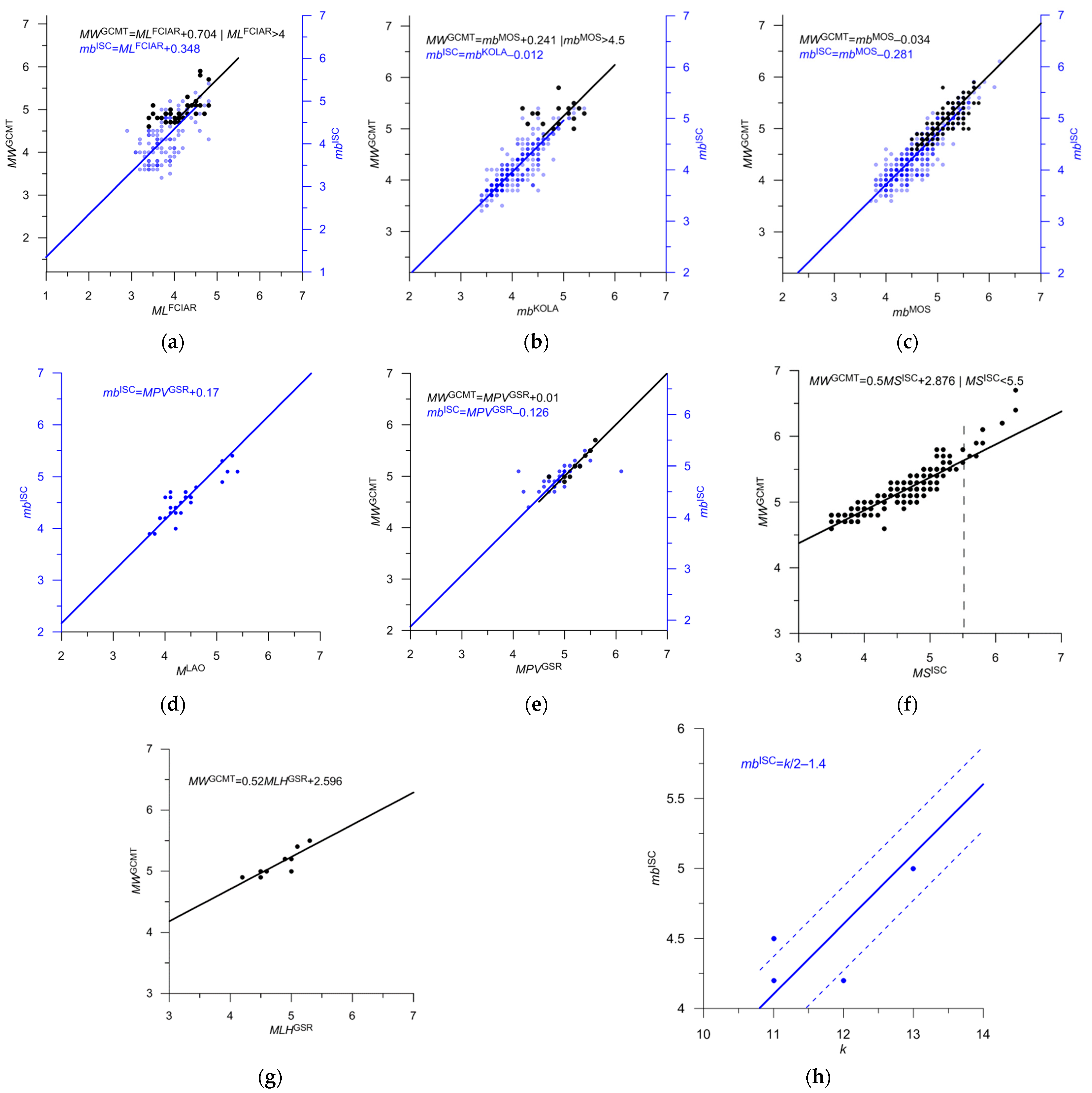
| FCIAR | ML | 3 | 561 | M = MLFCIAR + 0.6 | 0.37 | 19a | 2.0–4.3 | Gakkel |
| KOLA | mb | 4 | 32 | M = mbKOLA + 0.2 | 0.74 | 19b | 3.1–4.2 | Gakkel |
| MOS | mb | 4 | 1 | M = mbMOS | 0.82 | 19c | 5.3 | Gakkel |
| USCGS | mb | 4 | 2 | M = mbUSCGS + 0.2 | 0.83 | 18a | 3.8–4.0 | Gakkel and Knipovich |
| BER | Mw | 4 | 23 | M = MwBER − 0.1 | 0.72 | 16a | 3.1–4.1 | Gakkel and Knipovich |
| BER | mb(Pn) | 4 | 30 | M = mb(Pn)BER − 0.1 | 0.82 | 16b | 2.6–4.0 | Gakkel and Knipovich |
| BER | ML | 5 | 3 | M = MLBER + 1.2 | 0.54 | 15c | 1.9–2.3 | Knipovich, unreliable |
| DNK | ML | 5 | 3 | M = MLDNK + 0.6 | 0.79 | 16c | 1.7–2.3 | 2008–2015.2, Knipovich, unreliable |
| DNK | ML | 5 | 15 | M = MLDNK + 1.3 | 0.57 | 16d | 0.6–2.2 | 2015.3–2022, Knipovich, unreliable |
| KOLA | ML | 5 | 24 | M = MLKOLA + 0.5 | 0.65 | 16e | 1.3–3.5 | Knipovich, unreliable |
| NAO | ML | 4 | 3 | M = MLNAO + 1.1 | 0.53 | 16f | 2.4–2.8 | 1990–2008, Gakkel and Knipovich |
| LAO | M | 4 | 5 | M = MLAO + 0.4 | 0.79 | 19d | 3.7–4.5 | Gakkel |
| IDC | mb | 4 | 141 | M = mbIDC + 0.2 | 0.85 | 17c | 3.2–4.3 | Gakkel and Knipovich |
| EIDC | mb | 4 | 19 | M = mbEIDC + 0.3 | 0.76 | 17d | 2.7–3.9 | Gakkel and Knipovich |
| GSR | MPV | 4 | 2 | M = MPVGSR | 0.44 | 19e | 4.4–5.0 | Gakkel |
| ISC | MS | 4 | 1 | M = 0.5MSISC + 2.88 | 0.85 | 19f | 5.3 | Gakkel |
| GSR | MLH | 4 | 4 | M = 0.52MLHGSR + 2.6 | 0.75 | 19g | 3.0–3.4 | Gakkel |
| OTT | ML | 5 | 5 | M = MLOTT + 0.1 | 0.23 | 18e | 3.2–4.2 | Gakkel and Knipovich Poorly determined |
| GSR | k | 5 | 16 | M = k/2 − 1.2 | 0.51 | 19h | 9–11 | Gakkel Poorly determined |
| CSEM | ML | 5 | 2 | M = MLCSEM | – | 2.2–2.6 | Not Determined | |
| CGS | M | 5 | 2 | M = MCGS | – | 4.2–4.6 | Not Determined | |
| MSCGS | M | 5 | 1 | M = MMSCGS | – | 4.3 | Not Determined | |
| PAL | M | 5 | 2 | M = MPAL | – | 4.0–4.8 | Not Determined | |
| STU | M | 5 | 1 | M = MSTU | – | 4.8 | Not Determined | |
| Total | 2089 |
Disclaimer/Publisher’s Note: The statements, opinions and data contained in all publications are solely those of the individual author(s) and contributor(s) and not of MDPI and/or the editor(s). MDPI and/or the editor(s) disclaim responsibility for any injury to people or property resulting from any ideas, methods, instructions or products referred to in the content. |
© 2023 by the authors. Licensee MDPI, Basel, Switzerland. This article is an open access article distributed under the terms and conditions of the Creative Commons Attribution (CC BY) license (https://creativecommons.org/licenses/by/4.0/).
Share and Cite
Vorobieva, I.A.; Gvishiani, A.D.; Shebalin, P.N.; Dzeboev, B.A.; Dzeranov, B.V.; Sergeeva, N.A.; Kedrov, E.O.; Barykina, Y.V. Integrated Earthquake Catalog III: Gakkel Ridge, Knipovich Ridge, and Svalbard Archipelago. Appl. Sci. 2023, 13, 12422. https://doi.org/10.3390/app132212422
Vorobieva IA, Gvishiani AD, Shebalin PN, Dzeboev BA, Dzeranov BV, Sergeeva NA, Kedrov EO, Barykina YV. Integrated Earthquake Catalog III: Gakkel Ridge, Knipovich Ridge, and Svalbard Archipelago. Applied Sciences. 2023; 13(22):12422. https://doi.org/10.3390/app132212422
Chicago/Turabian StyleVorobieva, Inessa A., Alexei D. Gvishiani, Peter N. Shebalin, Boris A. Dzeboev, Boris V. Dzeranov, Natalia A. Sergeeva, Ernest O. Kedrov, and Yuliya V. Barykina. 2023. "Integrated Earthquake Catalog III: Gakkel Ridge, Knipovich Ridge, and Svalbard Archipelago" Applied Sciences 13, no. 22: 12422. https://doi.org/10.3390/app132212422
APA StyleVorobieva, I. A., Gvishiani, A. D., Shebalin, P. N., Dzeboev, B. A., Dzeranov, B. V., Sergeeva, N. A., Kedrov, E. O., & Barykina, Y. V. (2023). Integrated Earthquake Catalog III: Gakkel Ridge, Knipovich Ridge, and Svalbard Archipelago. Applied Sciences, 13(22), 12422. https://doi.org/10.3390/app132212422