


Research Method for Ship Engine Fault Diagnosis Based on Multi-Head Graph Attention Feature Fusion


Abstract
:1. Introduction
- (1)
- Transform the ship engine dataset into two graph structures from different scales and make the two graph structures contain similarity relationships from multiple perspectives by extracting the neighbor relationships between samples so as to achieve complementation and extension of the model input information.
- (2)
- Introducing fusion weights, the two graph structures are structurally fused according to appropriate weights to obtain a fused graph structure that contains deeper information.
- (3)
- Input the obtained fusion graph structure into the GANN of fused multi-head attention for multi-channel feature extraction, and finally connect the Softmax layer to realize fault diagnosis.
- (4)
- The ship engine thermal parameter dataset is used to verify that the MPGANN proposed in this paper outperforms other classical algorithms and achieves higher accuracy.
2. Related Work and Theory
2.1. Data Topology Construction
2.1.1. Probabilistic Graph Structure
2.1.2. Rank-Order Graph Structure
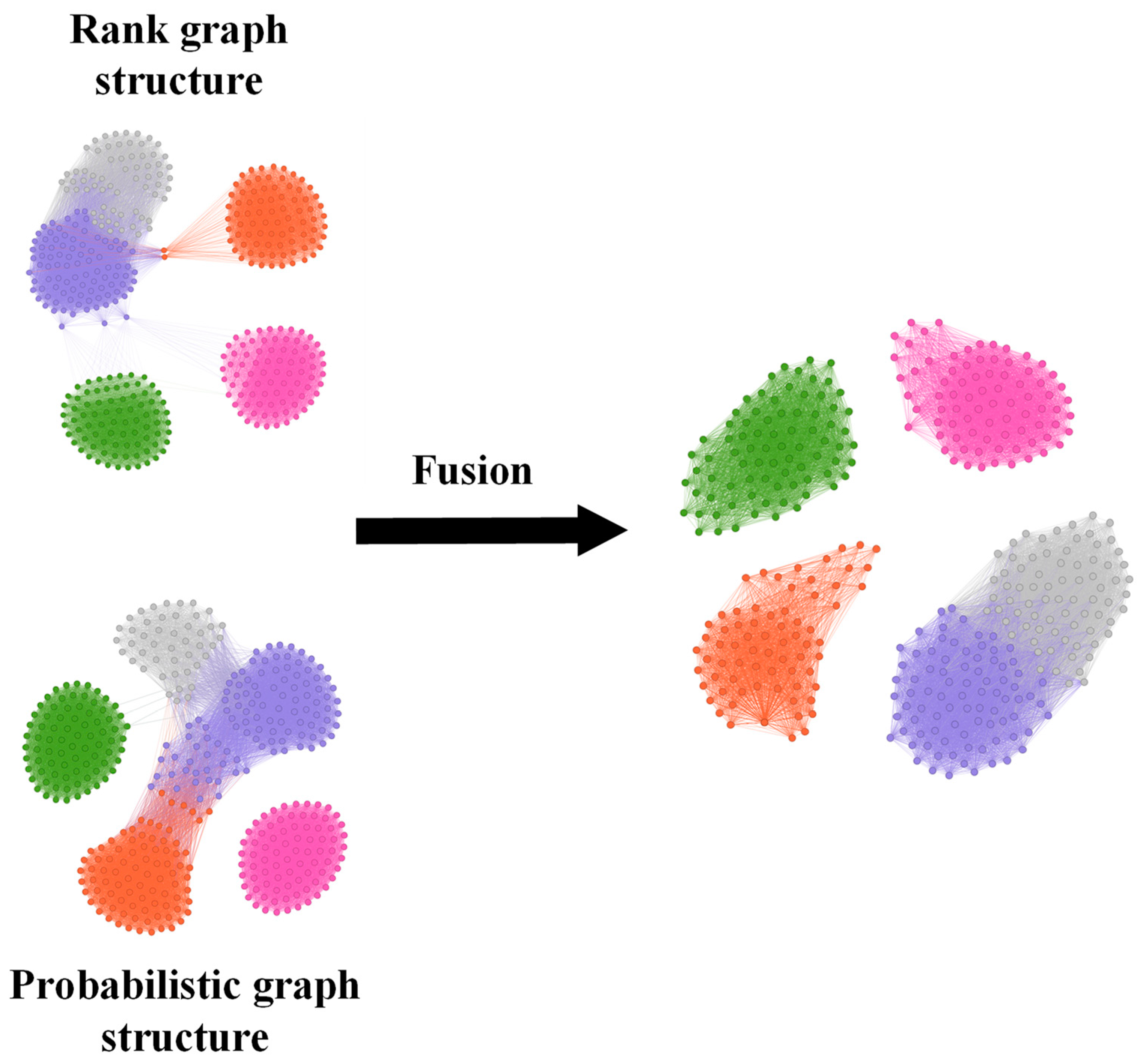
2.1.3. Feature Graph Fusion
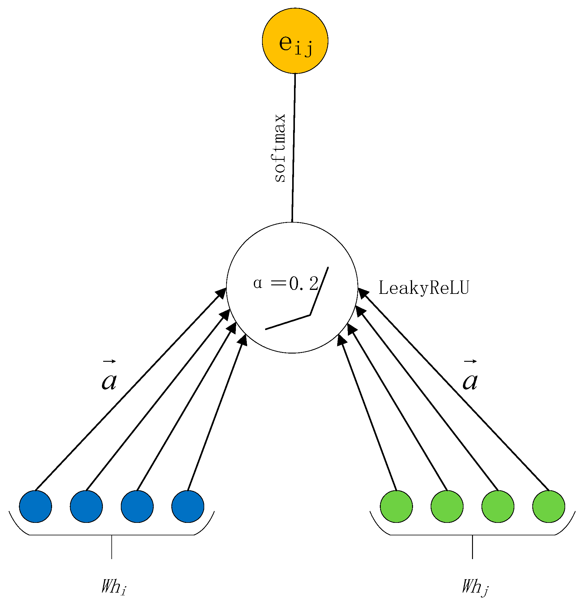
2.2. Graphical Attention Neural Network
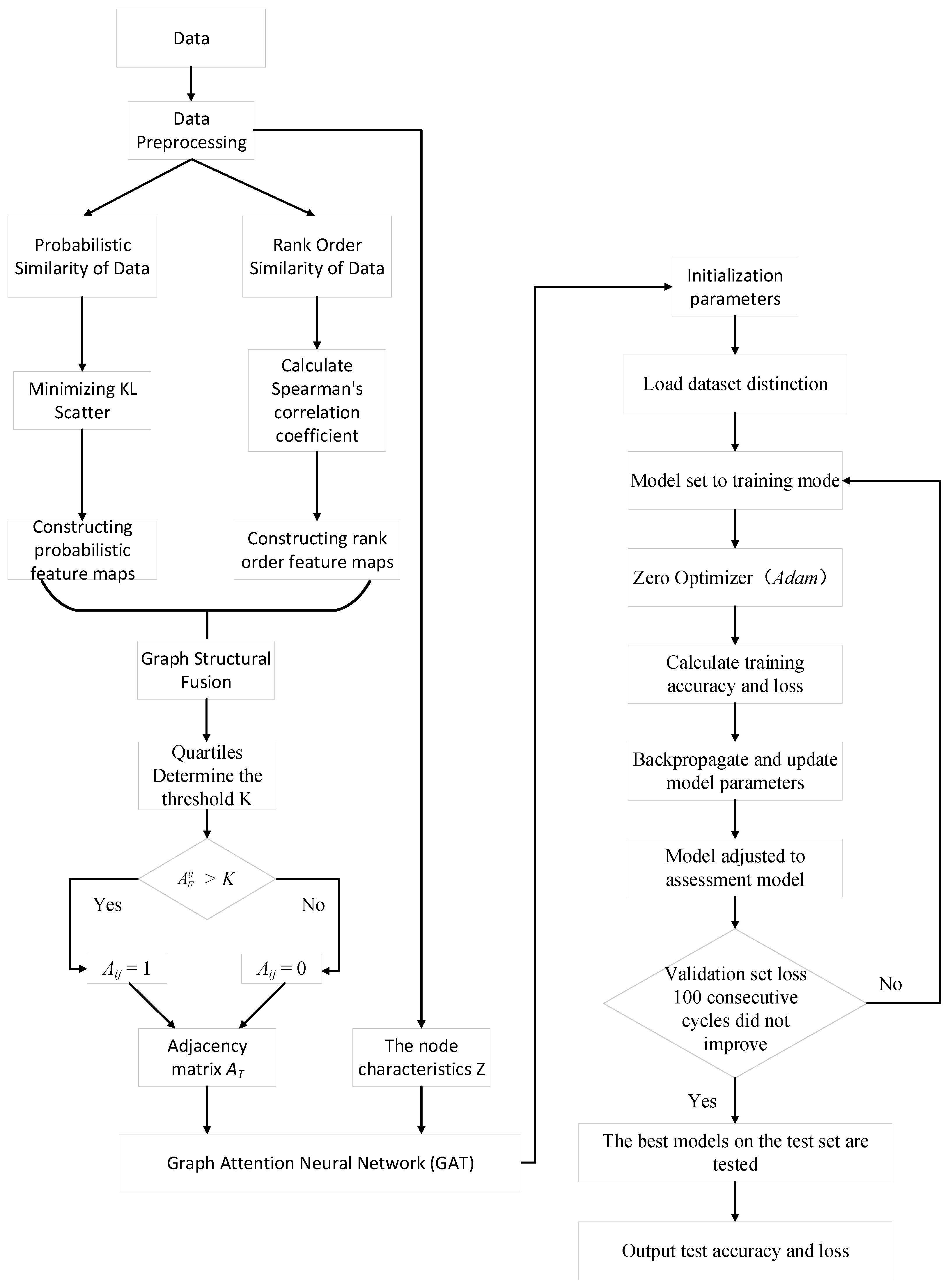
2.3. Algorithmic Process
3. Case Study
3.1. Data Description
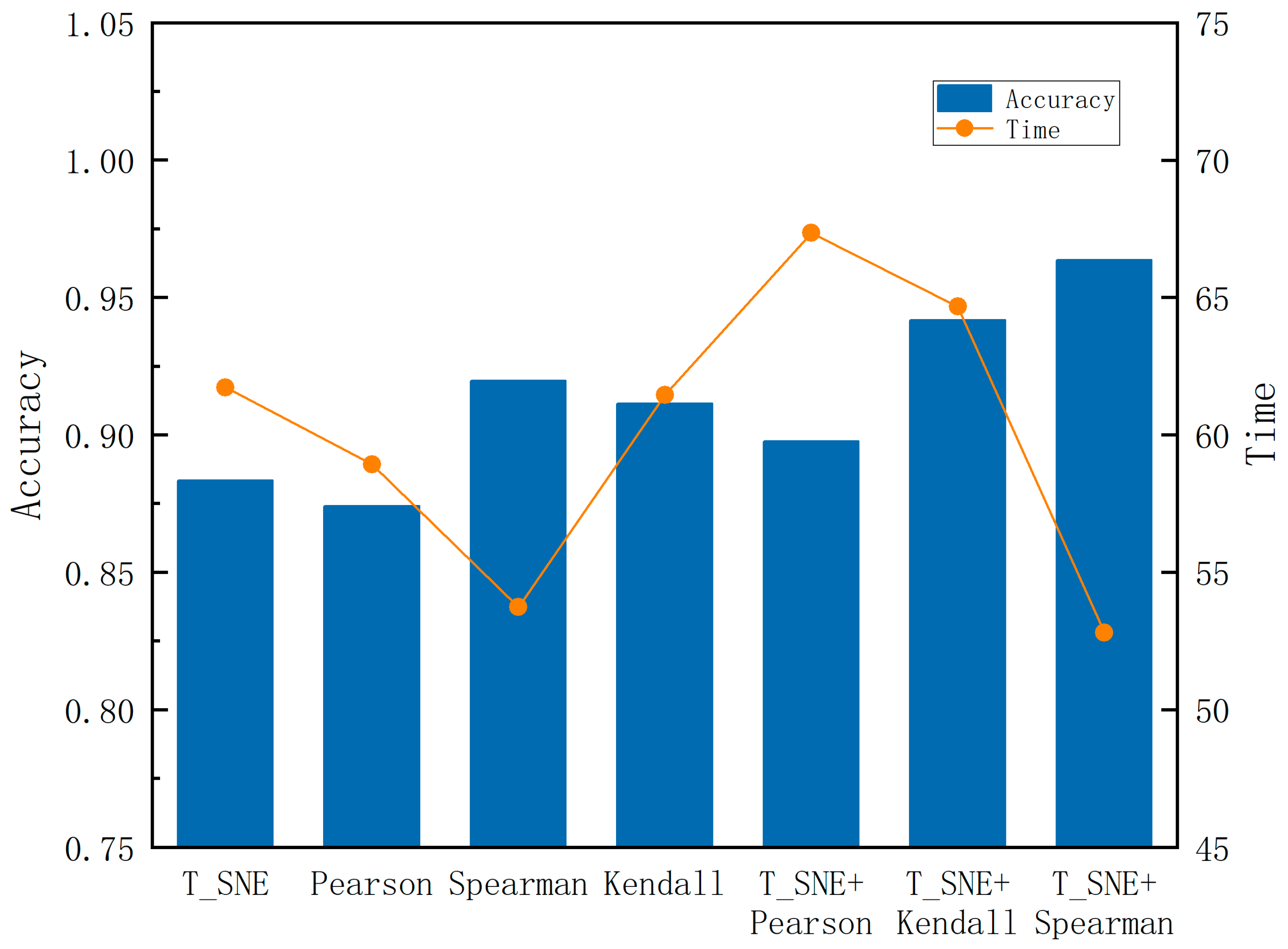
3.2. Comparison of Graph Structures
3.3. Network Parameter Setting
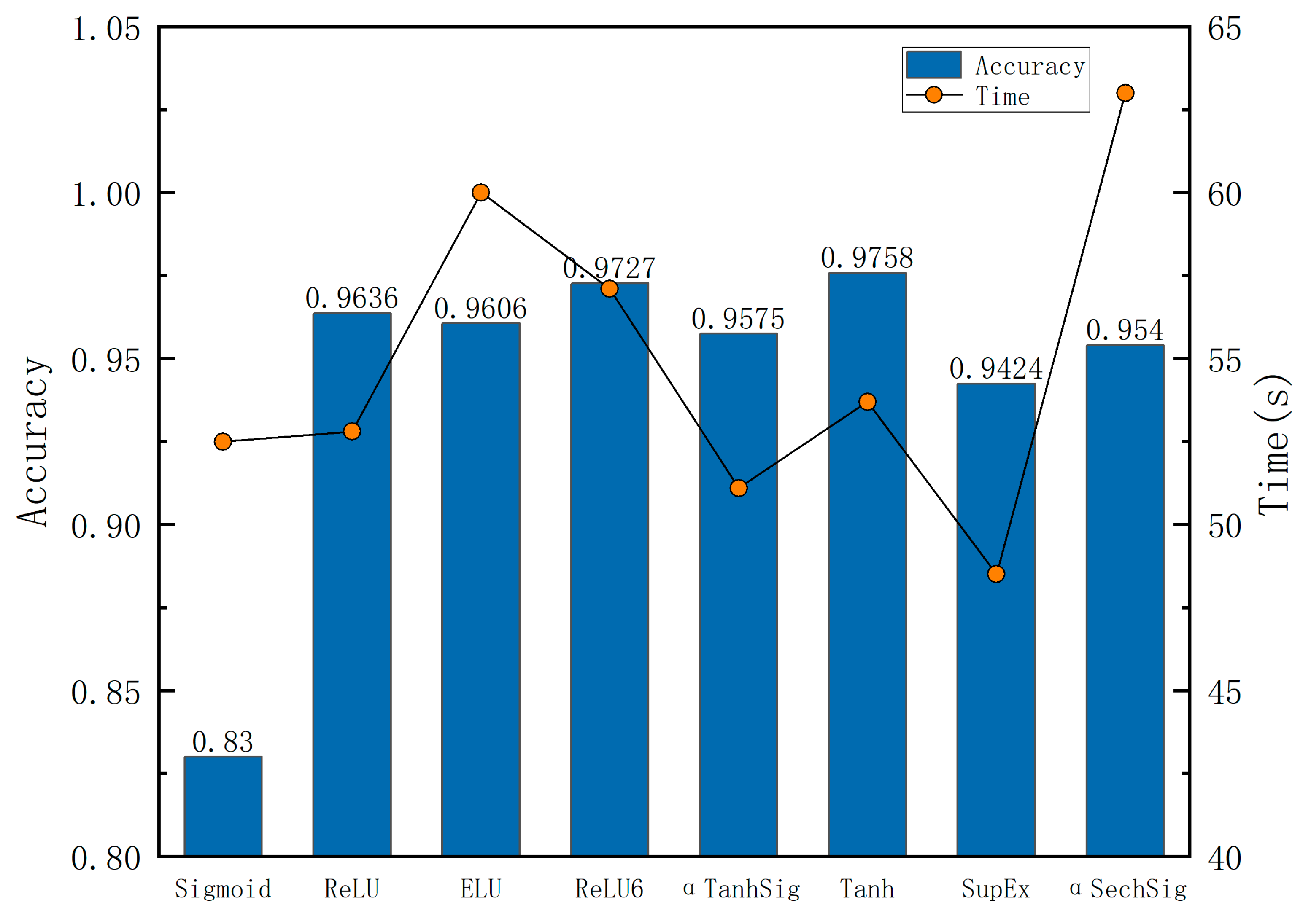
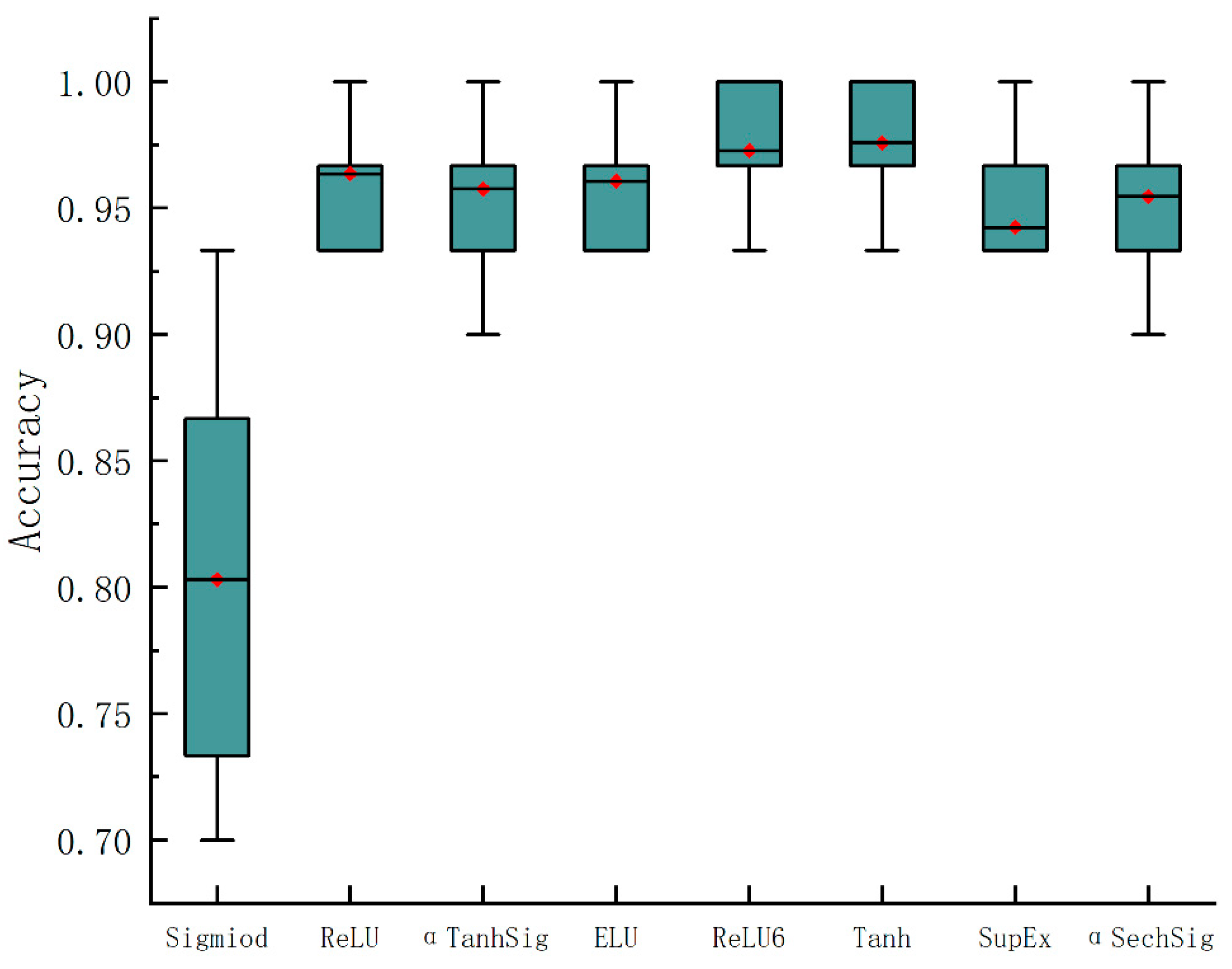
3.3.1. Activation Function
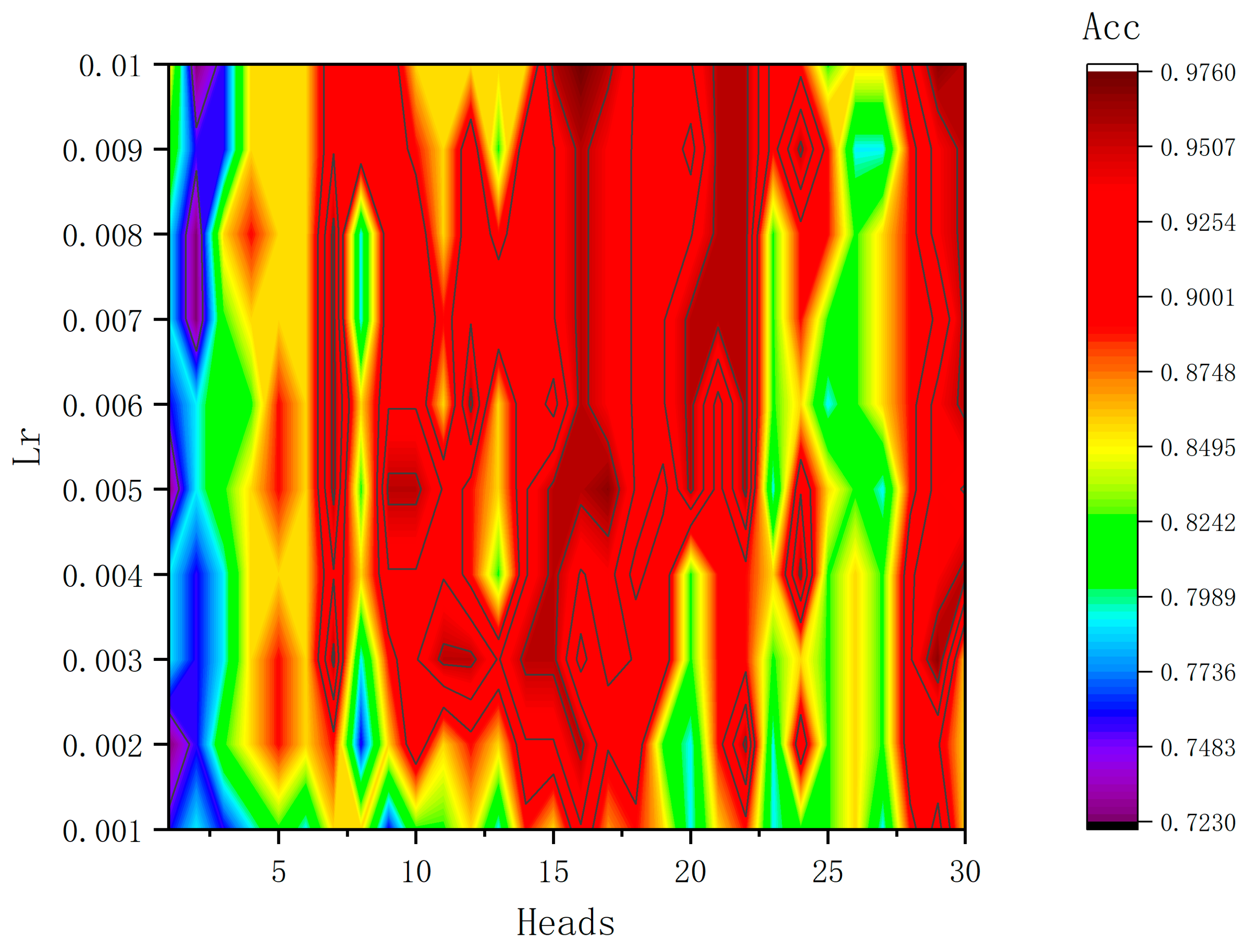
3.3.2. Number of Attention Heads
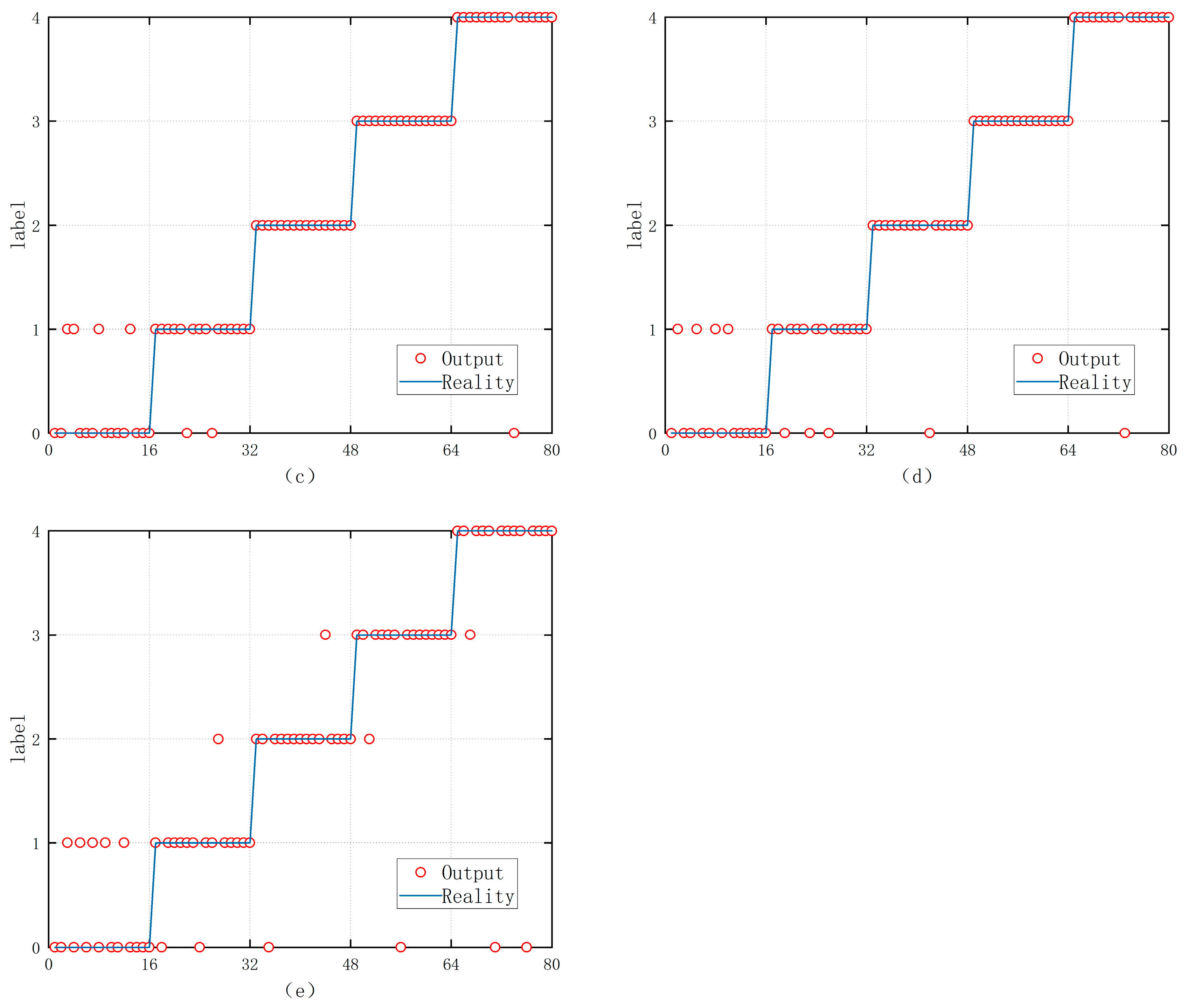
3.3.3. Algorithm Performance Comparison
4. Conclusions
- (1)
- The two graph structure construction methods in the MPGANN model can effectively obtain probabilistic similarity and ordinal similarity between data samples and transform the data into probabilistic graph structure and ordinal graph structure.
- (2)
- Early fusion is employed to combine the probability map structure and rank-order map structure with the incorporation of feature weights. This integration process effectively amalgamates information from samples at various scales.
- (3)
- The multi-head attention mechanism is applied to conduct multi-channel feature screening on the fusion graph structure, extracting feature information with higher relevance to enhance the diagnostic performance of the model.
- (4)
- The model effect was validated using the ship engine fault dataset, and compared with other models in terms of accuracy, precision, recall, and F1 score, MPGANN was the most effective, with a diagnostic accuracy as high as 97.58% and an F1 score of 97.6%.
Author Contributions
Funding
Institutional Review Board Statement
Informed Consent Statement
Data Availability Statement
Conflicts of Interest
References
- Zhong, G.Q.; Wang, H.Y.; Zhang, K.Y.; Jia, B.Z. Fault diagnosis of Marine diesel engine based on deep belief network. In Proceedings of the 2019 Chinese Automation Congress (CAC), Hangzhou, China, 22–24 November 2019; pp. 3415–3419. [Google Scholar] [CrossRef]
- Hou, L.; Zhang, J.; Du, B. A Fault Diagnosis Model of Marine Diesel Engine Fuel Oil Supply System Using PCA and Optimized SVM. J. Phys. Conf. Ser. 2020, 1576, 012045. [Google Scholar] [CrossRef]
- Zhong, K.; Li, J.B.; Wang, J.; Han, M. Fault Detection for Marine Diesel Engine Using Semi-supervised Principal Component Analysis. In Proceedings of the 9th International Conference on Information Science and Technology (ICIST), Hulunbuir, China, 2–5 August 2019; pp. 146–151. [Google Scholar]
- Ren, D.P.; Zeng, H.; Wang, X.L.; Pang, S.; Wang, J.D. Fault Diagnosis of Diesel Engine Lubrication System Based on Bayesian Network. In Proceedings of the 6th International Conference on Control, Automation and Robotics (ICCAR), Electr Network, Singapore, 20–23 April 2020; pp. 423–429. [Google Scholar]
- Han, P.H.; Li, G.Y.; Skulstad, R.; Skjong, S.; Zhang, H.X. A Deep Learning Approach to Detect and Isolate Thruster Failures for Dynamically Positioned Vessels Using Motion Data. IEEE Trans. Instrum. Meas. 2021, 70, 1–11. [Google Scholar] [CrossRef]
- Xu, X.J.; Zhao, Z.Z.; Xu, X.B.; Yang, J.B.; Chang, L.L.; Yan, X.P.; Wang, G.D. Machine learning-based wear fault diagnosis for marine diesel engine by fusing multiple data-driven models. Knowl. Based Syst. 2020, 190, 105324. [Google Scholar] [CrossRef]
- Cao, H.; Zhang, J.D.; Cao, X.; Li, R.; Wang, Y.R. Optimized SVM-Driven Multi-Class Approach by Improved ABC to Estimating Ship Systems State. IEEE Access 2020, 8, 206719–206733. [Google Scholar] [CrossRef]
- Wang, R.H.; Chen, H.; Guan, C. Random convolutional neural network structure: An intelligent health monitoring scheme for diesel engines. Measurement 2021, 171, 108786. [Google Scholar] [CrossRef]
- Memis, S.; Arslan, B.; Aydin, T.; Enginoglu, S.; Camci, C. Distance and Similarity Measures of Intuitionistic Fuzzy Parameterized Intuitionistic Fuzzy Soft Matrices and Their Applications to Data Classification in Supervised Learning. Axioms 2023, 12, 463. [Google Scholar] [CrossRef]
- Choo, K.B.; Cho, H.; Park, J.H.; Huang, J.F.; Jung, D.; Lee, J.; Jeong, S.K.; Yoon, J.; Choo, J.; Choi, H.S. A Research on Fault Diagnosis of a USV Thruster Based on PCA and Entropy. Appl. Sci. 2023, 13, 3344. [Google Scholar] [CrossRef]
- Zhao, N.Y.; Mao, Z.W.; Wei, D.H.; Zhao, H.P.; Zhang, J.J.; Jiang, Z.N. Fault Diagnosis of Diesel Engine Valve Clearance Based on Variational Mode Decomposition and Random Forest. Appl. Sci. 2020, 10, 1124. [Google Scholar] [CrossRef]
- Memis, S. Picture Fuzzy Soft Matrices and Application of Their Distance Measures to Supervised Learning Picture Fuzzy Soft k-Nearest Neighbor (PFS-kNN). Electronics 2023, 12, 4129. [Google Scholar] [CrossRef]
- Yang, K.; Fan, H.Y. Research on Fault Diagnosis Method of Diesel Engine Thermal Power Conversion Process. In Proceedings of the 3rd International Forum on Energy, Environment Science and Materials (IFEESM), Shenzhen, China, 25–26 November 2017; pp. 1445–1450. [Google Scholar]
- Agrawal, S.K.; Banerjee, S.; Sinha, A.; Das, D. SafeEngine: Fault Detection with Severity Prediction for Diesel Engine. In Proceedings of the 2022 IEEE 10th Region 10 Humanitarian Technology Conference (R10-HTC), Hyderabad, India, 16–18 September 2022; pp. 216–220. [Google Scholar]
- Zhou, J.; Cui, G.; Hu, S.; Zhang, Z.; Yang, C.; Liu, Z.; Wang, L.; Li, C.; Sun, M. Graph neural networks: A review of methods and applications. AI Open 2020, 1, 57–81. [Google Scholar] [CrossRef]
- Nie, J.; Xu, Y.; Huang, Y.; Li, J. The review of image processing based on graph neural network. In Proceedings of the International Conference on Intelligent Robotics and Applications, Yantai, China, 22–25 October 2021; pp. 534–544. [Google Scholar]
- Zhou, A.Z.; Li, Y.F. Structural attention network for graph. Appl. Intell. 2021, 51, 6255–6264. [Google Scholar] [CrossRef]
- Kipf, T.N.; Welling, M. Semi-supervised classification with graph convolutional networks. arXiv 2016, arXiv:1609.02907. [Google Scholar]
- Wang, R.; Chen, H.; Guan, C. DPGCN Model: A Novel Fault Diagnosis Method for Marine Diesel Engines Based on Imbalanced Datasets. IEEE Trans. Instrum. Meas. 2022, 72, 1–11. [Google Scholar] [CrossRef]
- Li, T.; Zhao, Z.; Sun, C.; Yan, R.; Chen, X. Domain adversarial graph convolutional network for fault diagnosis under variable working conditions. IEEE Trans. Instrum. Meas. 2021, 70, 1–10. [Google Scholar] [CrossRef]
- Zheng, J.; Gao, Q.; Lü, Y. Quantum graph convolutional neural networks. In Proceedings of the 2021 40th Chinese Control Conference (CCC), Shanghai, China, 26–28 July 2021; pp. 6335–6340. [Google Scholar]
- Veličković, P.; Cucurull, G.; Casanova, A.; Romero, A.; Lio, P.; Bengio, Y. Graph attention networks. arXiv 2017, arXiv:1710.10903. [Google Scholar]
- Yang, F.; Zhang, H.Y.; Tao, S.M. Semi-supervised classification via full-graph attention neural networks. Neurocomputing 2022, 476, 63–74. [Google Scholar] [CrossRef]
- Zhang, S.; Gong, H.; She, L. An aspect sentiment classification model for graph attention networks incorporating syntactic, semantic, and knowledge. Knowl. Based Syst. 2023, 275, 110662. [Google Scholar] [CrossRef]
- Van der Maaten, L.; Hinton, G. Visualizing data using t-SNE. J. Mach. Learn. Res. 2008, 9, 2579–2605. [Google Scholar]
- Zhang, W.-Y.; Wei, Z.-W.; Wang, B.-H.; Han, X.-P. Measuring mixing patterns in complex networks by Spearman rank correlation coefficient. Phys. A Stat. Mech. Appl. 2016, 451, 440–450. [Google Scholar] [CrossRef]
- Wang, Y.; Qin, Y.; Guo, J.; Cao, Z.; Jia, L. Multi-point short-term prediction of station passenger flow based on temporal multi-graph convolutional network. Phys. A Stat. Mech. Appl. 2022, 604, 127959. [Google Scholar] [CrossRef]
- Wang, L.; Hu, Z.; Kong, Q.; Qi, Q.; Liao, Q. Infrared and Visible Image Fusion via Attention-Based Adaptive Feature Fusion. Entropy 2023, 25, 407. [Google Scholar] [CrossRef] [PubMed]
- Luo, Z.; Li, J.; Zhu, Y. A deep feature fusion network based on multiple attention mechanisms for joint iris-periocular biometric recognition. IEEE Signal Process. Lett. 2021, 28, 1060–1064. [Google Scholar] [CrossRef]
- Yang, J.; Yang, J.-Y.; Zhang, D.; Lu, J.-F. Feature fusion: Parallel strategy vs. serial strategy. Pattern Recognit. 2003, 36, 1369–1381. [Google Scholar] [CrossRef]
- Wang, Y.; Xu, X.; Yu, W.; Xu, R.; Cao, Z.; Shen, H.T. Comprehensive Framework of Early and Late Fusion for Image–Sentence Retrieval. IEEE MultiMedia 2022, 29, 38–47. [Google Scholar] [CrossRef]
- Boulahia, S.Y.; Amamra, A.; Madi, M.R.; Daikh, S. Early, intermediate and late fusion strategies for robust deep learning-based multimodal action recognition. Mach. Vis. Appl. 2021, 32, 121. [Google Scholar] [CrossRef]
- Ruiz, L.; Gama, F.; Ribeiro, A. Graph neural networks: Architectures, stability, and transferability. Proc. IEEE 2021, 109, 660–682. [Google Scholar] [CrossRef]
- Brauwers, G.; Frasincar, F. A general survey on attention mechanisms in deep learning. IEEE Trans. Knowl. Data Eng. 2021, 35, 3279–3298. [Google Scholar] [CrossRef]
- Weston, J.; Chopra, S.; Bordes, A. Memory networks. arXiv 2014, arXiv:1410.3916. [Google Scholar]
- Kiliçarslan, S.; Közkurt, C.; Bas, S.; Elen, A. Detection and classification of pneumonia using novel Superior Exponential (SupEx) activation function in convolutional neural networks. Expert Syst. Appl. 2023, 217, 119503. [Google Scholar] [CrossRef]
- Közkurt, C.; Kiliçarslan, S.; Bas, S.; Elen, A. αSechSig and αTanhSig: Two novel non-monotonic activation functions. Soft Comput. 2023, 27, 18451–18467. [Google Scholar] [CrossRef]


| Working Condition | Form | Power/kW | Booster Outlet Pressure/Bar | Air Cooler Outlet Temperature/°C | Fuel Consumption/ g/Cycle |
|---|---|---|---|---|---|
| 100% load | simulation value | 4104.99 | 4.6732 | 46.6 | 4.14 |
| measured value | 4078 | 4.528 | 46 | 4.12 | |
| inaccuracies/% | 0.6618 | 1.1815 | 1.3043 | 0.4854 | |
| 75% load | simulation value | 3393.19 | 3.2067 | 42.9 | 3.17 |
| measured value | 3375 | 3.74 | 42 | 3.18 | |
| inaccuracies/% | 0.5390 | −2.1471 | 2.143 | −0.3145 | |
| 50% load | simulation value | 2295.03 | 2.3018 | 36.7 | 2.23 |
| measured value | 2250 | 2.57 | 38 | 2.24 | |
| inaccuracies/% | 2.001 | −3.4319 | −3.4211 | −0.4464 | |
| 25% load | simulation value | 1164.88 | 1.277 | 28.4 | 1.21 |
| measured value | 1125 | 1.42 | 29 | 1.26 | |
| inaccuracies/% | 3.5449 | −3.0282 | −2.0689 | −3.9683 | |
| Working Condition | Form | Inlet Flow/g/s | Average Effective Pressure/bar | Exhaust Temperature/°C | |
| 100% load | simulation value | 8370.9823 | 20.0947 | 455.3 | |
| measured value | 8300 | 19.96 | 460 | ||
| inaccuracies/% | 0.8552 | 0.6748 | −0.1022 | ||
| 75% load | simulation value | 6477.0966 | 17.4753 | 438.75 | |
| measured value | 6800 | 16.52 | 445 | ||
| inaccuracies/% | −3.2780 | 3.9667 | −1.4045 | ||
| 50% load | simulation value | 4249.7621 | 11.4935 | 437.8 | |
| measured value | 4600 | 11.01 | 430 | ||
| inaccuracies/% | −3.266 | 3.4518 | 1.8140 | ||
| 25% load | simulation value | 2371.3959 | 5.7910 | 427.7 | |
| measured value | 2600 | 5.51 | 410 | ||
| inaccuracies/% | −3.9848 | 3.5957 | 3.5593 | ||
| Malfunction Code | Parameterization | |||||
|---|---|---|---|---|---|---|
| Failure Characteristics | Regular Value | Degree of Failure | ||||
| LV1 | LV2 | LV3 | LV4 | |||
| F1 | Injection timing advance | −13.1 deg | −14.1 | −15.1 | −16.1 | −17.1 |
| F2 | Delayed injection timing | −13.1 deg | −12.1 | −11.1 | −10.1 | −9.1 |
| F3 | Decline in supercharger efficiency | 100% | 95% | 90% | 85% | 80% |
| F4 | Reduced air cooler efficiency | 100% | 95% | 90% | 85% | 80% |
| Working Condition | Dimension | Sample Size |
|---|---|---|
| Injection timing advance (F1) | 23 | 80 |
| Delayed injection timing (F2) | 23 | 80 |
| Decline in supercharger efficiency (F3) | 23 | 80 |
| Reduced air cooler efficiency (F4) | 23 | 80 |
| Normal operation (F5) | 23 | 80 |
| Notation | Monitoring Indicators | Unit | Notation | Monitoring Indicators | Unit |
|---|---|---|---|---|---|
| Pmp3 | Booster outlet pressure | bar | Tmp23 | Exhaust manifold temperature | °C |
| Vmp3 | Supercharger outlet flow | m/s | Pmp24 | Turbine outlet pressure | bar |
| Tmp3 | Supercharger inlet temperature | °C | Vmp24 | Turbine Outlet Flow | m/s |
| Pmp4 | Air cooler inlet pressure | bar | Tmp24 | Turbine outlet temperature | °C |
| Vmp4 | Air cooler outlet flow | m/s | F | Air intake | kg/s |
| Tmp4 | Air cooler outlet temperature | °C | g | Fuel consumption rate | g/kW·h |
| Pmp5 | Cylinder inlet pressure | bar | Pz | Maximum burst pressure | bar |
| Vmp5 | Cylinder inlet flow | m/s | λ | Maximum voltage rise | bar/deg |
| Tmp5 | Cylinder inlet temperature | °C | Ne | Power (output) | kW |
| Tmp14 | Cylinder exhaust temperature | °C | PI | IMEP | bar |
| Pmp23 | Exhaust manifold pressure | bar | PB | BMEP | bar |
| Vmp23 | Exhaust manifold flow | m/s | / | / | / |
| Algorithms | Precision | Recall | ||||||||
|---|---|---|---|---|---|---|---|---|---|---|
| F1 | F2 | F3 | F4 | F5 | F1 | F2 | F3 | F4 | F5 | |
| MPGANN | 1 | 0.89 | 1 | 1 | 1 | 0.88 | 1 | 1 | 1 | 1 |
| GCN | 0.88 | 0.884 | 0.94 | 1 | 1 | 0.88 | 0.94 | 1 | 0.94 | 0.94 |
| CNN | 0.8 | 0.78 | 1 | 1 | 1 | 0.75 | 0.88 | 1 | 1 | 0.94 |
| SVM | 0.71 | 0.76 | 1 | 1 | 1 | 0.75 | 0.81 | 0.94 | 1 | 0.94 |
| BPNN | 0.65 | 0.72 | 0.88 | 0.88 | 1 | 0.69 | 0.81 | 0.88 | 0.88 | 0.81 |
Disclaimer/Publisher’s Note: The statements, opinions and data contained in all publications are solely those of the individual author(s) and contributor(s) and not of MDPI and/or the editor(s). MDPI and/or the editor(s) disclaim responsibility for any injury to people or property resulting from any ideas, methods, instructions or products referred to in the content. |
© 2023 by the authors. Licensee MDPI, Basel, Switzerland. This article is an open access article distributed under the terms and conditions of the Creative Commons Attribution (CC BY) license (https://creativecommons.org/licenses/by/4.0/).
Share and Cite
Ai, Z.; Cao, H.; Wang, J.; Cui, Z.; Wang, L.; Jiang, K. Research Method for Ship Engine Fault Diagnosis Based on Multi-Head Graph Attention Feature Fusion. Appl. Sci. 2023, 13, 12421. https://doi.org/10.3390/app132212421
Ai Z, Cao H, Wang J, Cui Z, Wang L, Jiang K. Research Method for Ship Engine Fault Diagnosis Based on Multi-Head Graph Attention Feature Fusion. Applied Sciences. 2023; 13(22):12421. https://doi.org/10.3390/app132212421
Chicago/Turabian StyleAi, Zeren, Hui Cao, Jihui Wang, Zhichao Cui, Longde Wang, and Kuo Jiang. 2023. "Research Method for Ship Engine Fault Diagnosis Based on Multi-Head Graph Attention Feature Fusion" Applied Sciences 13, no. 22: 12421. https://doi.org/10.3390/app132212421
APA StyleAi, Z., Cao, H., Wang, J., Cui, Z., Wang, L., & Jiang, K. (2023). Research Method for Ship Engine Fault Diagnosis Based on Multi-Head Graph Attention Feature Fusion. Applied Sciences, 13(22), 12421. https://doi.org/10.3390/app132212421