Saturation-Based Airlight Color Restoration of Hazy Images

Abstract

Typically, images captured in adverse weather conditions such as haze or smog exhibit light gray or white color on screen; therefore, existing hazy image restoration studies have performed dehazing under the same assumption. However, hazy images captured under actual weather conditions tend to change color because of various environmental factors such as dust, chemical substances, sea, and lighting. Color-shifted hazy images have hindered accurate color perception of the images, and due to the dark haze color, they have worsened visibility compared to conventional hazy images. Therefore, various color correction-based dehazing algorithms have recently been implemented to restore colorcast images. However, existing color restoration studies are limited in that they struggle to distinguish between haze and objects, particularly when haze veils and images have a similar color or when objects with a high saturation value occupy a significant portion of the scene, resulting in overly grayish images and distorted colors. Therefore, we propose a saturation-based dehazing method that extracts only the hue of the cast airlight and preserves the information of the object. First, the proposed color correction method uses a dominant color extraction method for the clustering of CIELAB(LAB) color images and then assigns area scores to the classified clusters. Sorting of the airlight areas is performed using the area score, and gray world-based white balance is performed by extracting the hue of the area. Finally, the saturation of the restored image is used to separate and process the distant objects and airlight, and dehazing is performed by applying a weighting value to the depth map based on the average luminance. Our color restoration method prevents excessive gray tone and color distortion. In particular, the proposed dehazing method improves upon existing issues where near-field information is lost and noise is introduced in the far field as visibility improves.

1. Introduction

Scene analysis, target tracking, remote detection systems, and other outdoor image-based systems are affected by adverse atmospheric conditions caused by floating particles such as haze, clouds, or smog. Outdoor images and videos captured under bad weather often suffer from reduced visibility, low contrast, distorted colors, and low illumination intensity, which can degrade their quality and impact the performance of these systems. Therefore, researchers have conducted extensive studies to restore hazy images captured in adverse weather conditions [1,2,3,4,5,6,7,8].

Typically, atmospheric particles such as fog and smog manifest as white or grayish colors in scenes, and previous research assumed this coloration and performed dehazing accordingly. However, hazy images captured under real-world weather conditions often exhibit color variations due to various environmental factors such as sand, chemical substances, sea, noise, and lighting conditions [9,10,11,12]. Color-shifted hazy images have hindered the accurate color perception of scenes, and the intense coloration of dense haze has often resulted in worse visibility compared with standard hazy images. Consequently, conventional dehazing methods [1,2,3,4,5,6,7,8] failed to restore the color of color-cast real hazy images, often producing distorted color. Therefore, unlike typical hazy images, real hazy images have presented greater challenges in dehazing due to color-cast issues.

Color correction-based dehazing algorithms have been proposed to restore color-cast images such as sandstorm images and underwater scenes. To address the issue of blurred visibility, Koschmieder’s atmospheric scattering model (ASM) [13,14] has been used as a popular single-image dehazing method [1,2,3,4,5,6]. ASM effectively defined various hazy images that required color correction, not limited to typical hazy images, and was used for various dehazing tasks, including underwater images [15,16,17,18], sandstorm images [19,20,21], and color-cast remote detection images [22].

As He et al. proposed a dark channel prior (DCP) effective in removing haze, visibility restoration studies for various color-cast images have been conducted based on DCP [17,18,19,20,21]. Li et al. [17] effectively restored underwater images by calculating the difference between the dark channel priors of green and blue channels and the red channel prior. Shi et al. proposed halo-reduced dark channel prior dehazing (HRDCP) in which DCP was applied to the CIELAB(LAB) color space [20] to minimize the color distortion issue of the dehazing algorithm. Furthermore, Shi et al. proposed normalized gamma transformation-based contrast-limited adaptive histogram equalization (NGCCLAHE) [21] as a revised method for compensating the insufficient contrast improvement function of HRDCP by applying a gamma correction formulation to contrast limited adaptive histogram equalization (CLAHE) [23], a well-known contrast improvement method. Both HRDCP and NGCCLAHE efficiently restored color-cast hazy images using the gray world hypothesis for white balancing. In addition, various other dehazing methods apply color constancy to the images [15,16,17,22,24]. Among them, weighted scene depth adaptive color constancy (WSDACC) [22] effectively removed color cast in heavily affected images by correcting the loss of ambient light extinction in the medium as an image formation model.

However, existing color restoration studies have failed to consider the characteristics of haze models affected by ambient light, resulting in unsatisfactory results in some images. For example, color cast due to weather, scenes, or ambient light may exhibit colors similar to haze veils; however, existing methods are unable to address this, leading to output images with excessive grayscale or distorted colors. Furthermore, in cases where colorful objects occupy a wide area, distinguishing between the color of the haze and the objects is challenging, thereby posing limitations to existing methods.

Therefore, we propose a saturation-based dehazing method that preserves the information of objects by extracting only the hue of cast airlight. The proposed method addresses the existing color distortion issue by using the LAB color space in color correction and dehazing. First, the proposed color correction method uses a dominant color output method to cluster LAB color images and assign area scores to the classified clusters. These scores are used to identify the airlight areas, and the hue of the corresponding areas is detected to perform gray world-based white balancing. Furthermore, using the correlation between the luminance and saturation of the image and the depth of haze from the corrected image, this method generates a depth map equation. To address the loss of near-field information and the generation of far-field noise as visibility improves, this method uses the saturation of the restored image to separate and process far-field objects from airlight and applies a weighting value to the depth map based on the average luminance. The parameters of the defined depth map were estimated using multiple linear regression according to the linear characteristics and applied to the ASM for dehazing. The proposed method prevents excessive grayscale and color distortion while preserving object colors, thus improving upon the limitations of existing color restoration-based dehazing methods.

The remaining structure of this paper is as follows. Section 2 discusses theories related to color restoration, and Section 3 describes the proposed dehazing method. Section 4 presents the experimental results and discussions, comparing our method with existing methods. Finally, Section 5 concludes the paper.

2. Dehazing for Color Restoration

2.1. Atmospheric Scattering Model

ASM, or Koschmieder’s optical model [13,14], is widely used to restore blurred images in image processing research. ASM defines a hazy image $I\left(x\right)$ as follows:

$$I\left(x\right)=J\left(x\right)t\left(x\right)+A\left(1-t\left(x\right)\right)$$

(1)

$$t\left(x\right)=e^{-\beta d\left(x\right)}$$

(2)

where $x$ is the spatial coordinate of the scene, $t\left(x\right)$ is the transmission of the scene, $A$ is airlight, and $J\left(x\right)$ is the scene without haze. Also, $\beta$ in Equation (2) is a scattering coefficient, and $d\left(x\right)$ is the depth of the scene. In Equation (1), $J\left(x\right)t\left(x\right)$ represents direct decay, and $A\left(1-t\left(x\right)\right)$ represents the airlight area. $t\left(x\right)$ shows an exponential decay with distance $d\left(x\right)$ according to Equation (2). Therefore, if the distance between the observer and the scene is very long, the transmission rate $t\left(x\right)\approx 0$, and according to the definition of ASM, the direct decay area represents 0, while $A$ has a value very close to $I\left(x\right)$. This can be shown in the following equation:

$$I\left(x\right)\approx A\left(\mathrm{\infty }\right), d\left(x\right)\to \mathrm{\infty }, t\left(x\right)\to 0$$

(3)

Here, $A\left(\mathrm{\infty }\right)$ shows the entire area of the background airlight with infinitely large $d\left(x\right)$. Generally, since the sky area is the farthest from the object, $A\left(\mathrm{\infty }\right)$ can be considered as the atmospheric particles containing most of the haze information. Based on Equation (1), dehazing involves obtaining $J\left(x\right)$ by estimating $A$ and $t\left(x\right)$.

2.2. Gray World Hypothesis

When only the aforementioned ASM is used, the biased haze color can degrade the color recognition of the image, and the dark haze color may also degrade visibility. Therefore, many dehazing methods for color-cast images restore image color based on the gray world hypothesis [15,20,21,22].

The gray world hypothesis indicates that in a typical RGB color image, the average of each color channel is identical. Given that the R, G, and B channel values of a color-cast image $I\left(x\right)$ are $I_r\left(x\right)$, $I_g\left(x\right)$, and $I_b\left(x\right)$, and the white balance result is $\widehat{I_r}{\displaystyle \left(x\right)},\widehat{I_g}\left(x\right),$ and $\widehat{I_b}{\displaystyle \left(x\right)}$, respectively, the gray world hypothesis is expressed as follows [25,26]:

$$\begin{array}{c}\begin{array}{l}\widehat{I_r}\left(x\right)=\frac{G_{avg}}{R_{avg}}{I}_r\left(x\right)\\ \widehat{I_g}\left(x\right)=I_g\left(x\right)\end{array}\\ \widehat{I_b}\left(x\right)=\frac{G_{avg}}{B_{avg}}{I}_b\left(x\right)\end{array}$$

(4)

Given that the widths of the row and column of $I\left(x\right)$ are $M$ and $N$, respectively, the average $R_{avg}$, $G_{avg}$, and $B_{avg}$ of the R, G, and B channels can be expressed as follows:

$$\begin{array}{c}\begin{array}{l}{R}_{avg}=\frac{1}{MN}{\displaystyle \sum _{X=1}^{MN}}{I}_r\left(x\right)\\ G_{avg}=\frac{1}{MN}{\displaystyle \sum _{X=1}^{MN}}{I}_g\left(x\right)\end{array}\\ B_{avg}=\frac{1}{MN}{\displaystyle \sum _{X=1}^{MN}}{I}_b\left(x\right)\end{array}$$

(5)

The resulting images of the gray world hypothesis from the aforementioned Equations (4) and (5) can be verified in Figure 1.

In Figure 1, the typical hazy image produces a result very similar to the original image, as shown in Figure 1a,c. In contrast, the color-cast image shows a biased histogram, as shown in Figure 1b, and the gray world hypothesis restores color by moving and overlapping the corresponding histogram, as shown in Figure 1d.

Figure 1. Histogram of the gray world hypothesis: (a) normal hazy image, (b) color-cast hazy image, (c) restored normal image, and (d) restored color-cast image.

2.3. Gray World Hypothesis in the LAB Color Space

As discussed above, the gray world hypothesis restores color by correcting the reduced R, G, and B channels. However, because the RGB channel also contains the luminance of the image, Equation (4) can cause another color distortion due to excessive white balancing. Therefore, to address this issue with RGB images, the gray world hypothesis using LAB color space has been proposed [20,21].

CIELAB stands for a three-dimensional color space consisting of three channels, L, a, and b. The L channel represents the brightness component, and the a and b channels represent the saturation components. In particular, the a and b channels allow for the linear process as they are expressed on a grid: the negative value in the a channel is in green, and the positive value is in red; and the negative value in the b channel is blue, and the positive value is in yellow. In other words, higher values of a and b result in a stronger reddish or yellowish color cast, while a typical gray world has values of a and b close to 0.

Based on the characteristics of LAB, as shown in Equation (6), white balancing in the LAB color space can be performed. Because the saturation and luminance channels are separated in the LAB color space, Equation (6) does not affect L, resulting in little color distortion.

$$\begin{array}{c}\widehat{a}\left(x\right)=a\left(x\right)-a_{avg}\\ \widehat{b}\left(x\right)=b\left(x\right)-b_{avg}\end{array}$$

(6)

Here, $a\left(x\right)$ and $b\left(x\right)$ represent the $a$ and $b$ channel values in LAB, respectively, and $a_{avg}$ and $b_{avg}$ are the averages of $a\left(x\right)$ and $b\left(x\right)$.

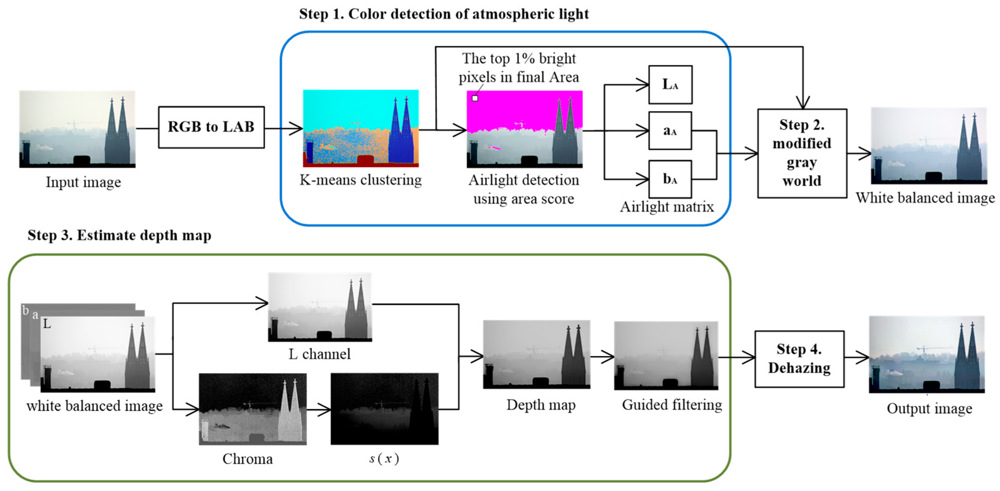
3. Proposed Dehazing Method

A flowchart of the proposed method is shown in Figure 2. As shown in Figure 2, the proposed dehazing method incorporates the following four stages: extraction of color components in airlight, improved hazy color correction based on the gray world hypothesis, depth map setting based on luminance and saturation, and dehazing. Since both color correction and dehazing in this study used the LAB color space, the RGB color space was first converted into the LAB color space to perform the color correction algorithm, and the color-corrected image was used as an input image for dehazing to estimate the depth map for the LAB color space. The estimated depth map restored the L channel through the ASM, and the restored L, a, and b channels were converted to the RGB color space for the final output.

Figure 2. Visualized flowchart of the proposed method.

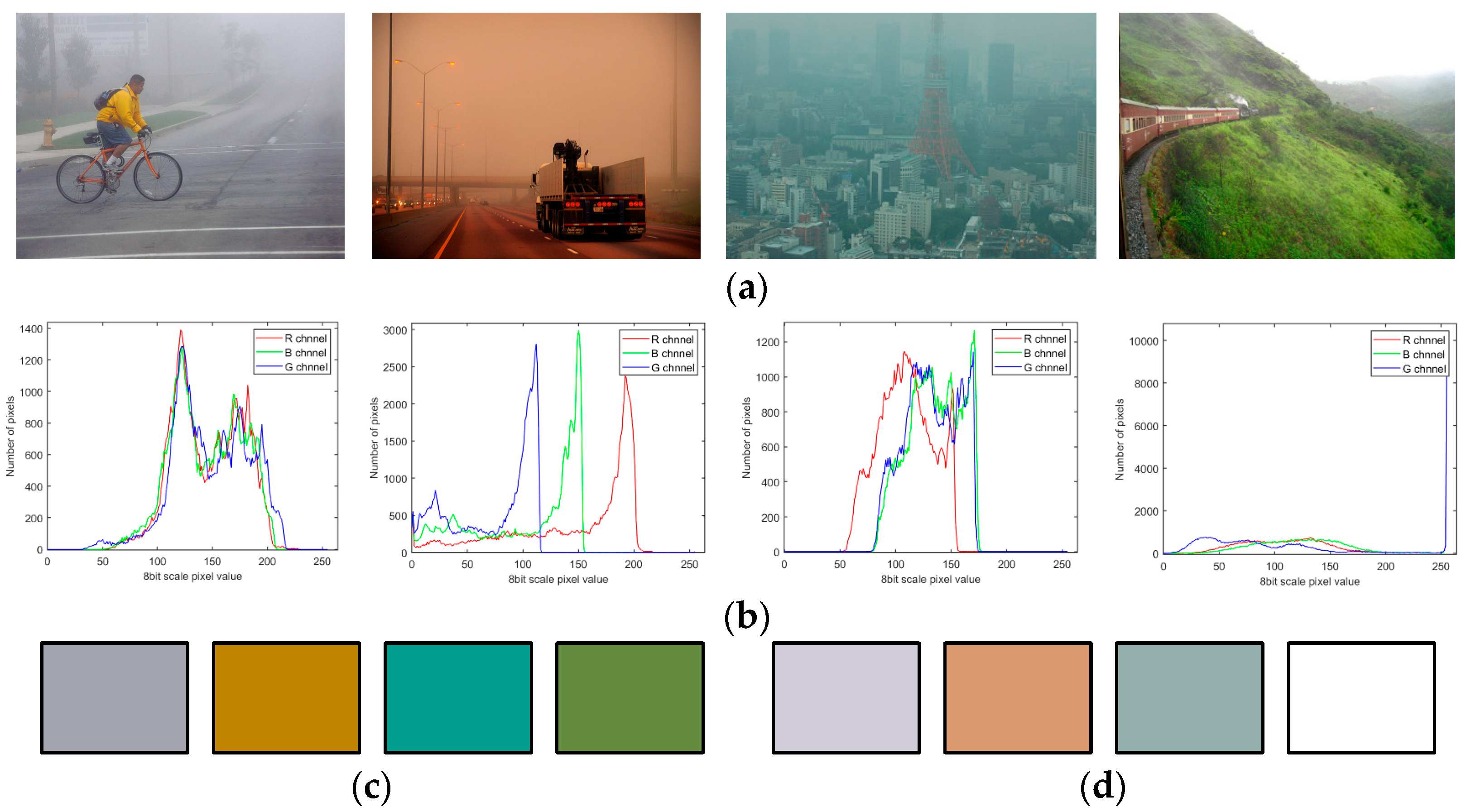
3.1. Extraction of Color Components in Airlight

Because the entire background airlight $A\left(\mathrm{\infty }\right)$ in a hazy image comprises bright pixels, the brightest pixels are generally aligned, and their average is considered to be airlight [1,2,3,4,5,6]. However, when there are objects in the image that have white as their inherent color, this method can include information from these objects rather than just the airlight. In particular, in the case of the L channel, which represents the luminance of the image, this method can result in even less reliable airlight extraction results.

Therefore, the proposed method to prevent such an error shows a way to output airlight by using the method which extracts the dominant color. The most dominant color extraction methods [27,28,29] use the K-means algorithm in CIELAB, an RGB color space. In recent research, Chang [29] defined the following hypotheses based on the analysis of color palette datasets:

• In most cases, the number of dominant colors is between 3 and 6.
• High saturation colors are often selected, with the most vivid colors almost always being chosen.
• The color that occupies the largest area is almost always chosen, regardless of its conspicuousness.
• When multiple colors are somewhat conspicuous, there is a greater likelihood that other colors will be chosen.
• Colors that differ significantly from the surrounding environment are more likely to be chosen.

In this study, clustering is performed by applying that algorithm to most hazy images; the sky area is dominant, and the sky can be differentiated from objects into Chang’s hypotheses 3 and 5. In particular, hypothesis 3 suggests that when the number of clusters k is small, the range may not include large areas, so an appropriate k should be chosen. The results depending on K are described in Section 3.1.2. In addition, Figure 3b,c show the results of the conventional airglow detection method and the proposed method.

Figure 3a shows the clustering result of the image, and Figure 3b,c show the results from the existing airlight extraction method and proposed method, respectively. In Figure 3, the pink area represents the extracted airlight area.

In this study, to perform the algorithm, the RGB image is first converted to the LAB color space in Section 3.1.1, and Section 3.1.2 and Section 3.1.3 explain the proposed airlight hue extraction method.

Figure 3. Airlight extraction using area division: (a) clustering of the hazy image with the sky, (b) extraction of the brightest pixels in the L channel, and (c) airlight area extraction using the proposed method.

3.1.1. Execution of the LAB Color Space Conversion Equation

To execute the proposed method, the LAB color space conversion equation is used to convert the entered RGB image into the CIELAB color space. The well-known LAB color space conversion equation is shown below [20,21].

$$\begin{array}{c}\begin{array}{l}L=116f\left(\frac{Y}{Y_n}\right)-16\\ a=500\left[f\left(\frac{X}{X_n}\right)-f\left(\frac{Y}{Y_n}\right)\right]\end{array}\\ b=200\left[f\left(\frac{Y}{Y_n}\right)-f\left(\frac{Z}{Z_n}\right)\right]\end{array}$$

(7)

Here,

$$\left[\begin{array}{c}X\\ Y\\ Z\end{array}\right]=\left[\begin{array}{ccc}0.4124& 0.3576& 0.1804\\ 0.2127& 0.7152& 0.0722\\ 0.0193& 0.1192& 0.9502\end{array}\right]\left[\begin{array}{c}R\\ G\\ B\end{array}\right]$$

(8)

$$f\left(q\right)=\left\{\begin{array}{l}\sqrt[3]{q},\hspace{1em}\hspace{1em} q>0.008856\\ 7.787q+\frac{4}{29},\hspace{1em} q\le 0.008856\end{array}\right.$$

(9)

$$X_n=95.047,Y_n=100.000,Z_n=108.883$$

(10)

Here, R, G, and B are the pixel values of the R, G, and B channels, respectively, and L, a, and b are the pixel values of the L, a, and b channels, respectively. Further, $X_n$, $Y_n$, and $Z_n$ are the tricolor stimulation values of the reference white light in the CIE XYZ color space.

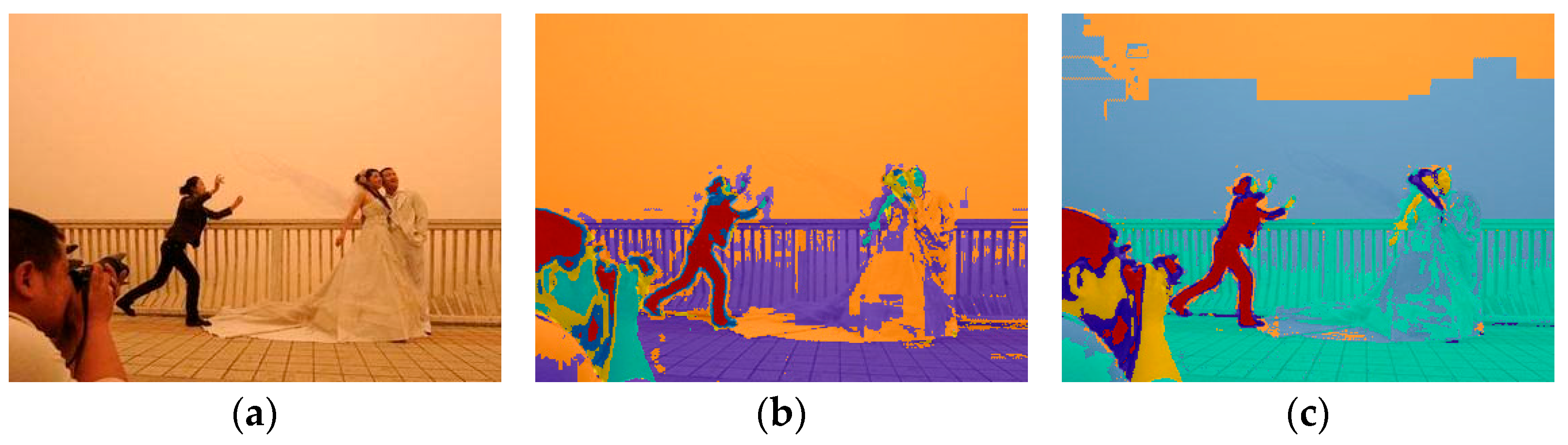
3.1.2. Division of the Image Using K-Means Clustering

The well-known K-means clustering is a non-training-based method that forms a cluster by placing k arbitrary central points on the closest objects. It is expressed as follows:

$${argmin}_S\sum _{i=1}^k\sum _{x\in S_i}^{}{‖x-{\mu }_i‖}^2$$

(11)

where $x$ is the data, $S$ is a cluster, $\mu$ is the average of the cluster components, and $k$ is the number of clusters. To execute K-means according to Equation (11), the number of clusters $k$ and the data with which sorting is performed $x$ must be established.

Generally, K-means algorithms for dominant color output in the CIELAB color space [28,29] use the saturation channels a and b of the image as input data. However, if an object with an achromatic color is present, it will form the same cluster as the airglow because its a and b values are almost identical. Also, if there is a color cast across the scene, the difference in the saturation of the entire image may be small and clustering may be less effective.

Accordingly, this study sets the input value as follows:

• The whole LAB color image from Equation (7) is used as the input image.
• The number of clusters “k” is set to 6 for better separation of bright objects.
• The number of repetitions is 3, which is the default value of the algorithm.
• K-means is initialized using cluster centroid initialization and the squared Euclidean distance measurement method.

In this paper, we segmented the images based on the K-means++ algorithm, and all k values were set to 6, which is the number that satisfies Chang’s first hypothesis.

K, the number of clusters, affects the detection results for the sky area. Unlike traditional saturation-based methods, the proposed method uses the LAB color channel, which bases clusters on shading and saturation differences. We measured the proposed method for k = 3–9 and found that when k is small, the objects in the fog image are detected in the same cluster as the sky area. Conversely, for a large k, sky areas are detected in multiple clusters. The experimental results show that the optimal value of k is 6, so we used k = 6 for clustering in this paper.

Based on the designed value, K-means clustering is performed to divide the LAB color image. The clustering results are shown in Figure 4, which also compares the saturation channel-based K-means and the proposed method.

Figure 4. Clustering results of the color-cast image: (a) original hazy image, (b) clustering using only a and b channels, and (c) clustering using the LAB color image.

Figure 4a,b show the sky area in the orange cluster area. However, Figure 4b also contains objects with low saturation; therefore, the proposed method is more favorable for separating the sky area.

3.1.3. Airlight Extraction Based on Area Scores

As shown in Figure 4, the clustering area sorted in Section 3.1.2 selects the optimal sky area by calculating the area score of these clusters. The sky area shows bright pixels in the image [1,2,3,4,5,6] with very low scattering [30]. Further, it has a relatively low saturation value compared with neighboring areas due to floating particles [5,31]. In this paper, the sky area consists of a set of bright, low variance, and low saturation pixels.

When the mean and variance of the L channel of the clustered group and the mean of the a and b channels are given as $\mu \left(L_i\right)$, $\sigma \left(L_i\right)$, and $\mu \left(\mu \left(a_i\right),\mu \left(b_i\right)\right)$, they represent the brightness, variance, and saturation of the clusters, respectively. First, $\mu \left(L_i\right)$ represents the mean of the L channel, so the larger the $\mu \left(L_i\right)$, the larger the brightness value of the sample pixels in the cluster. Second, $\sigma \left(L_i\right)$ represents the distribution of brightness values, signifying the distribution of pixels in the cluster. Finally, the $\mu \left(\mu \left(a_i\right),\mu \left(b_i\right)\right)$ represents the mean of the saturation channels, and the higher the value, the more saturated the cluster. Therefore, ${score}_i$, the area score for airglow estimation, is defined by Equation (12).

$$\begin{gathered} {score}_i=\mu \left(L_i\right)-\sigma \left(L_i\right)-\mu \left(\mu \left(a_i\right),\mu \left(b_i\right)\right) \\ i=1,\dots ,k \end{gathered}$$

(12)

Here, $\mu (·)$ and $\sigma (·)$ represent the average and scattering values of each cluster. Based on the characteristics of the sky area, the cluster with the highest value of ${score}_i$ is selected as the airlight area. The selected airlight area is shown in Figure 3c. As shown in Figure 3c, the selected airlight area is dominant in the image; thus, the top 1% of the pixels in this cluster are selected as the final airlight $A$, and their L, a, and b channel averages of the final airlight are entered into the 1 × 3 airlight matrix.

3.2. Improved Haze Color Correction Based on the Gray World Hypothesis

The existing color restoration methods are based on the gray world hypothesis, and color consistency and white balance are performed by adjusting the color average. However, depending on the scene, original images without additional hues may show a biased histogram. This can be observed through histograms and color means, as shown in Figure 5.

Figure 5. Veil color in various types of hazy images: (a) original images, (b) histogram of the original images, (c) average colors of the original images, and (d) airlight colors of the original images.

In Figure 5, when colorful objects dominate a wide range, the image exhibits a biased histogram. In such cases, the gray world hypothesis, as shown in Figure 5c, can perceive incorrect colors and perform excessive white balance [32]. This can be improved through the saturation of $A\left(\mathrm{\infty }\right)$, as shown in Figure 5d.

The saturation of $A\left(\mathrm{\infty }\right)$ shows a value very similar to the hue added in the image. Accordingly, the proposed method restores the color-cast image using the saturation value of $A\left(\mathrm{\infty }\right)$ to the gray world hypothesis. Given that the $a$ and $b$ channel values of the airlight matrix extracted in Section 3.1 are $a_A$ and $b_A$, respectively, the proposed method calculates the corrected colors $\widehat{a_A}\left(x\right)$ and $\widehat{b_A}\left(x\right)$ based on Equation (6).

$$\begin{array}{c}\widehat{a_A}\left(x\right)=a\left(x\right)-{wa}_A\\ \widehat{b_A}\left(x\right)=b\left(x\right)-{wb}_A\end{array}$$

(13)

In Equation (13), $w$ is the constant that shows the level of white balance and is set to $0.95~1$. Weight $w$ has a value of [0 1], and as $w$ increases, the image becomes closer to grayscale. In this paper, we use a $w$ of 0.95 for all datasets to carry out white balance.

3.3. Depth Map Setting Based on Luminance and Saturation

3.3.1. Depth Map of Haze Based on Existing Studies

The relation of a depth map to the saturation and luminance of a hazy image has already been proven in previous studies [5,31] using linear models. Accordingly, the depth map in the LAB channel can be expressed in a linear model as shown below.

$$d\left(x\right)=a_1+a_{2}L\left(x\right)+a_3\left(\left|a\left(x\right)\right|+\left|b\left(x\right)\right|\right)+{ϵ}_0$$

(14)

In this equation, saturation is expressed as $\left|a\right|+\left|b\right|$; $a_1$, $a_2$, and $a_3$ indicate the parameters for linear representation of the depth map. In addition, $\epsilon \left(x\right)$ is a random error that can be calculated using a Gaussian distribution model, $N(0,{\sigma }^2)$, where the average is 0 and the scattering is $\sigma$ [5].

$$d\left(x\right)~p\left(d\left(x\right)|x,a_0,a_1,a_2,{\sigma }^2\right)=N(a_1+a_{2}L+a_3\left(\left|a\right|+\left|b\right|\right),{\sigma }^2)$$

(15)

The multiple linear regression model satisfies $\epsilon ~N\left(0,{\sigma }^2\right)$ by the normality of the errors and has an expected value of zero. This causes the conditional expected value of the output to mean $a_1+a_{2}L+a_3\left(\left|a\right|+\left|b\right|\right)$, the $d\left(x\right)$ formula without the error term. $\sigma$, $N\left(0,{\sigma }^2\right)$’s input value, can be computed by the embedded multiple linear regression algorithm. Based on previous studies [5,31], a depth map has a strong correlation with the luminance and saturation of an image. Therefore, this study estimated the parameters $a_1$, $a_2$, and $a_3$ using multilinear regression, as presented Algorithm 1.

Algorithm 1. Parameter estimation algorithm using multilinear regression.

Input dataset

Depth map: 450 depth map datasets on NYU ground truth images

L, C, a, b: 450 L, $\left|a\right|+\left|b\right|$, a, b channel NYU images calculated from Section 3.1.1

Output: $\sigma$ for parameters $a_1$, $a_2$, $a_3$, and the normal distribution of the residual zone

Begin

for index = 1:450

Constant matrix with its component only at x1 = 1; x2 = L(index); x3 = C(index);

X = [x1 x2 x3]; Y = depth map(index);

Perform the multilateral regression algorithm using X as the input and Y as the output.

Enter the parameter and scattering of the corresponding index output to the 1, 2, 3, 4

columns of the output matrix $l$.

End

If a value with $R^2\le 0.5$ exists, the corresponding data are deleted.

Calculate the average of the final data on the output $l$, and $a_1$, $a_2$, $a_3$, $\sigma$.

End

To estimate the parameters in Equation (14), a depth map of a fog-free image is required as a dataset. Thus, we use the NYU dataset included in the D-Hazy dataset [33] as a sample. The NYU dataset provides depth maps of the hazy and ground truth images for each of the 450 fog images. For each of the collected NYU datasets, the values of L, a, b, and $\left|a\right|+\left|b\right|$ are computed and are set as the input value X for the multiple linear regression. When setting the depth map to the output Y, according to Equation (14), the estimated parameters are output as the matrix $l$ of size $450\times 4$, and the final parameters are computed by averaging $l$.

Equations (14) and (15) can effectively estimate the depth map using only a simple linear equation. However, because the same equation is applied to the entire region, the performance of restoring visibility for nearby objects’ shading or distant scene visibility is still unsatisfactory. Therefore, this study introduces weights reflecting saturation characteristics, as explained in Section 3.3.2.

3.3.2. Depth Map with the Saturation Weight

Scenes in distant areas create dark shading and noise as visibility increases [5,32]. Hazy images contain scenes that require visibility due to atmospheric light; thus, a method to distinguish between the sky area and objects is needed to address this. This study uses the color-restored saturation of a and b channels as the method for differentiating haze and objects.

The proposed method is explained in more detail in the saturation map shown in Figure 6. The saturation used the $\left|a\right|+\left|b\right|$ value, multiplied by 10, to visualize the noise in the sky area.

Figure 6. Saturation map for the color-restored hazy image: (a) color-restored input image, (b) 20-times amplified saturation map, and (c) saturation map of the hazy image multiplied by the weighting value $(L\left(x\right)-{\mu }_w)$.

In Figure 6, the color-restored input image shows the acromatic airlight area mostly via Equation (13). As a result, the airlight area shows the darkest value, and as shown in Figure 6b, airlight and objects can be separated by the color of the objects. Based on this assumption, the saturation map applied with the weighting value $s\left(x\right)$ is proposed as follows.

$$s\left(x\right)=(L\left(x\right)-{\mu }_w)(\left|a\left(x\right)\right|+\left|b\left(x\right)\right|)$$

(16)

Here, ${\mu }_w$ is the average of the $L$ channel of the white-balanced total image, showing the standard by which to differentiate close and distant objects. $s\left(x\right)$ outputs a positive value against the distant scene, whose luminance is higher than ${\mu }_w$, and a negative value against the close scene, whose luminance is smaller than ${\mu }_w$. As a result, Equation (16) performs stronger dehazing as it is closer to airlight, and dehazing with a smaller weighting value is performed on close objects susceptible to shading.

Since the saturation of the sky area results in a very low value close to 0, based on the assumption of the saturation of the sky area, the multiplication of $s\left(x\right)$ and saturation in a distant scene leaves only the hazy object components except the sky area. The multiplication of $s\left(x\right)$ and saturation is shown in Figure 6c, which was amplified 10 times for visualization.

As explained, this study sets $d\left(x\right)$ based on luminance and saturation as follows:

$$d\left(x\right)=a_1+a_{2}L\left(x\right)+a_{3}s\left(x\right)+{ϵ}_0$$

(17)

$s\left(x\right)$ in Equation (17) is the saturation applied with the weighting value set in Equation (16). All parameters in Equation (17), $a_1$, $a_2$, and $a_3$, and scattering $\sigma$ can be calculated by resetting the input value x3 as $s\left(x\right)C$ in Algorithm 1, and the random error ${ϵ}_0$ can be calculated by applying the calculated scattering $\sigma$ to Equation (15).

Because of executing Equation (17) in Algorithm 1, the values $a_1=-0.2138$, $a_2=0.9103$, $a_3=1.3970$, and $\sigma =0.0224$ were obtained, and $\sigma$ was used to generate random error ${ϵ}_0$, for each location $x$, through the Gaussian distribution model described in Equation (15). This study uses all of these parameters as generalized parameters for all hazy images. Meanwhile, Figure 6b,c show some noise, and to remove it, we performed guide filtering [3].

The proposed depth map estimation, as explained above, is performed as follows:

• Retrieve the L, a, and b channels of the image resulting from the restoration presented in Section 3.2 and define their pixel values as $L\left(x\right)$, $a\left(x\right)$, and $b\left(x\right)$.
• $\sigma =0.0224$ is applied to the Gaussian distribution model of Equation (15), $N(0,{\sigma }^2)$, to produce the random error ${ϵ}_0$ to each location $x$.
• Enter these into Equation (17) using $a_1=-0.2138$, $a_2=0.9103$, $a_3=1.3970$, and ${ϵ}_0$ to estimate $d\left(x\right)$, the depth map to which the weighting value of saturation is applied.
• To solve the noise of the saturation map, filtering is performed using the guide filter on $d\left(x\right)$.

Figure 7 illustrates the depth map and the corresponding guide filtering results.

Figure 7. Depth map of the proposed method: (a) estimated depth map and (b) depth map applied with guide map.

3.4. Dehazing

We detected the airglow $A\left(\mathrm{\infty }\right)$ through Section 3.1 and restored the color of the image through Section 3.2, and we estimated the depth of the fog $d\left(x\right)$ in Section 3.3. Thus, $t\left(x\right)$ and $J\left(x\right)$ can be obtained using the ASM equation.

Fog images captured in bad weather are more affected by noise than normal images due to the influence of suspended particles. The resulting image $J\left(x\right)$ is more susceptible to noise and more noise can occur when the transmission rate $t\left(x\right)$ value approaches 0 or 1. To avoid this noise, we set $t\left(x\right)$ in the range of 0.05 to 0.95 [5,7,8,9,10]. Using about 200 different fog image datasets, we measured the range from 0 to 1 on both sides in 0.01 decrements, with the best overall results obtained between 0.05 and 0.95.

$$t\left(x\right)=max(0.05,\mathit{min}(0.95,e^{-\beta d\left(x\right)}))$$

(18)

The aforementioned output $A\left(\mathrm{\infty }\right)$ and $t\left(x\right)$ in Equation (18) are entered into ASM Equation (1). To prevent color distortion, the L channel, which shows only luminance, is set to input image $I\left(x\right)$ and used in the ASM equation.

$$J\left(x\right)=\frac{L\left(x\right)-L_A}{t\left(x\right)}+L_A$$

(19)

In Equation (19), $L_A$ is the L value of the airlight matrix $A$, $A\left(\mathrm{1,1}\right);$ $J\left(x\right)$ is a grayscale image. To obtain an RGB image, the L, $\widehat{a_A}$, and $\widehat{b_A}$ values are substituted in the $J$, a, and b values of the LAB color space conversion equation. The equation for converting the LAB color space to the RGB space is shown below [18,19].

$$\left\{\begin{array}{c}\begin{array}{l}X=X_n{f}^{-1}\left( \frac{J+16}{116}+\frac{\widehat{a_A}}{500} \right)\\ Y=Y_n{f}^{-1}\left( \frac{J+16}{116} \right)\end{array}\\ Z=Z_{n}200\left( \frac{J+16}{116}-\frac{\widehat{b_A}}{200} \right)\end{array}\right.$$

(20)

$$\left[\begin{array}{c}R\\ G\\ B\end{array}\right]=\left[\begin{array}{ccc}3.2410& -1.5374& -0.4986\\ -0.9692& 1.8760& 0.0416\\ 0.0556& -0.2040& 1.0570\end{array}\right]\left[\begin{array}{c}X\\ Y\\ Z\end{array}\right]$$

(21)

In Equation (19), $f^{-1}\left(q\right)$ is the inverse function of $f\left(q\right)$ in Equation (9); $X_n$, $Y_n$, and $Z_n$ show values identical to those in Equation (10).

The guide filter applied in Figure 7 can reduce the contrast of the image somewhat because it smooths out the edge area based on the original image [5,31]. To solve this issue, the well-known contrast improvement technique CLAHE [23] was applied to an RGB image previously produced for correction. In this study, to prevent supersaturation of the image, the contrast improvement limit of CLAHE was set to 0.03–0.05. CLAHE’s contrast enhancement limit has a range of [0 1]. The proposed algorithm was simulated for various fog images in 0.01 increments, and the best overall characteristics were obtained at 0.03.

4. Experimental Results and Discussions

This paper uses a desktop with an intel Core i5-2400 CPU (3.1GHz) and 4GB memory as a test platform and runs the algorithms in MATLAB R2023a. In this study, recent studies on color-added hazy images, HRDCP [20], NGCCLAHE [21], and WSDACC [22], were compared with the proposed method to assess its performance. While HRDCP and NGCCLAHE have often been used for dust dehazing, the authors showed that they performed well for general hazy images and color-cast images. The proposed method and the existing methods were visually evaluated in Section 4.1 and objectively evaluated in Section 4.2.

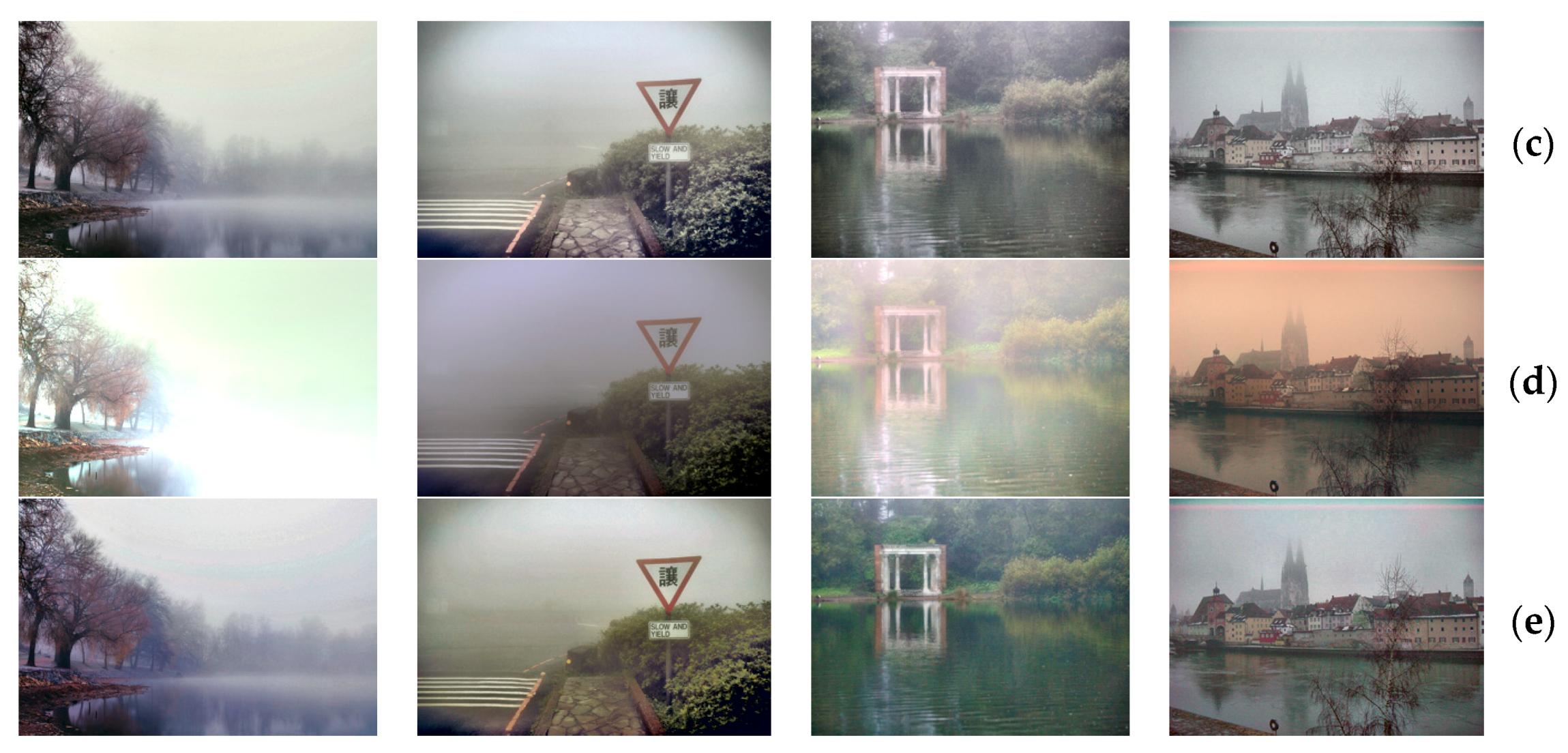
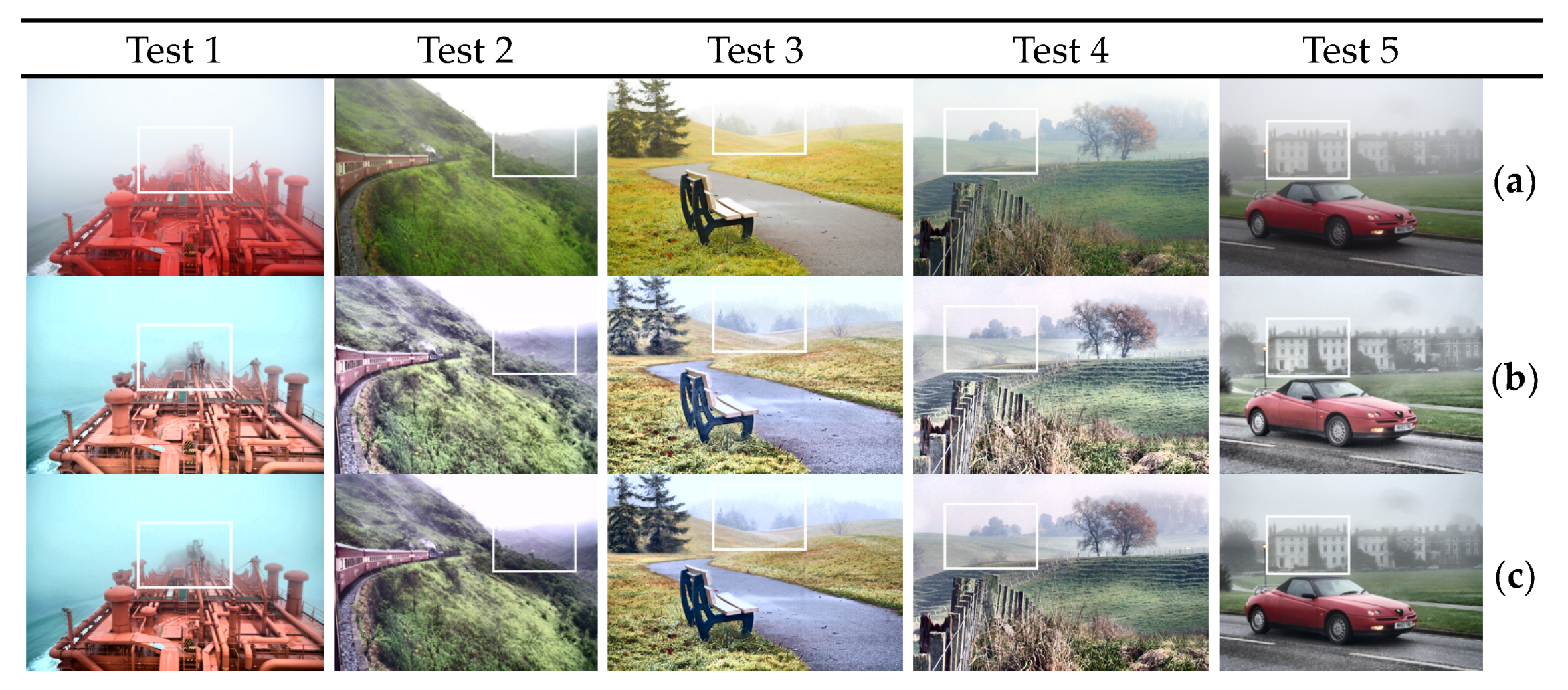
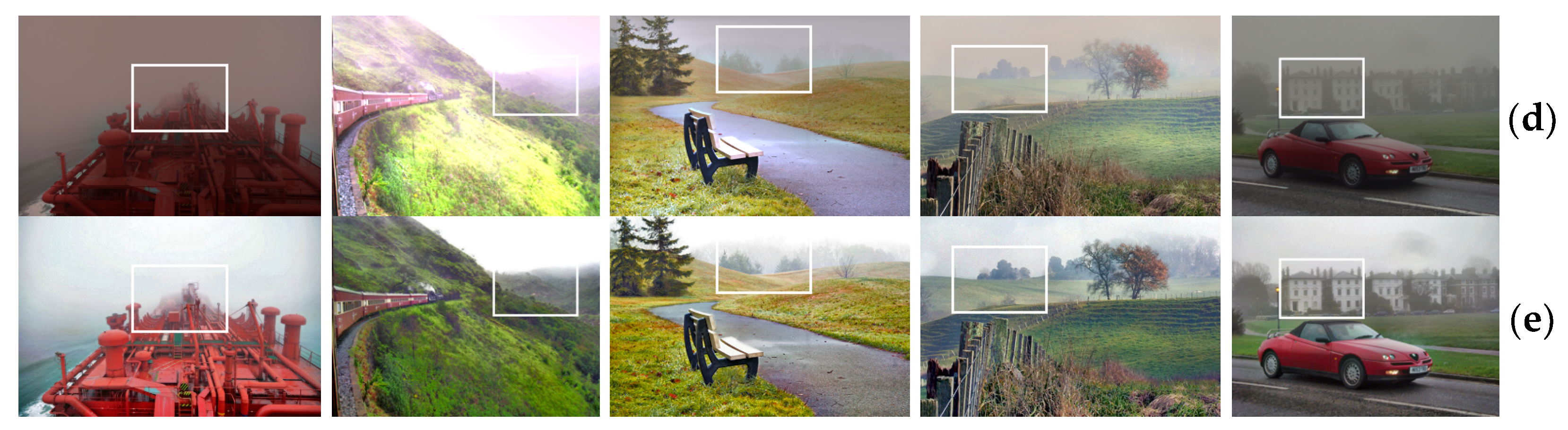
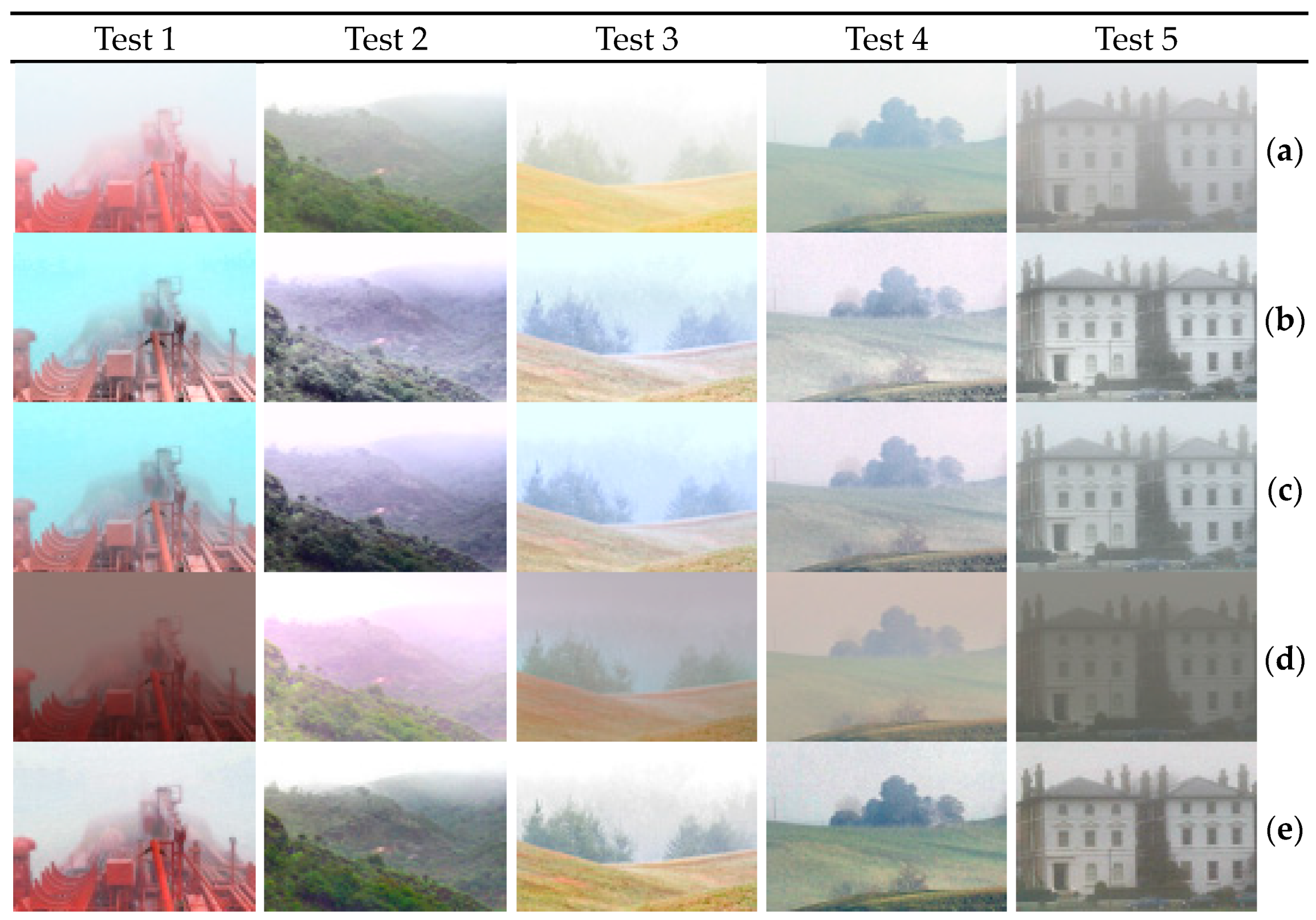
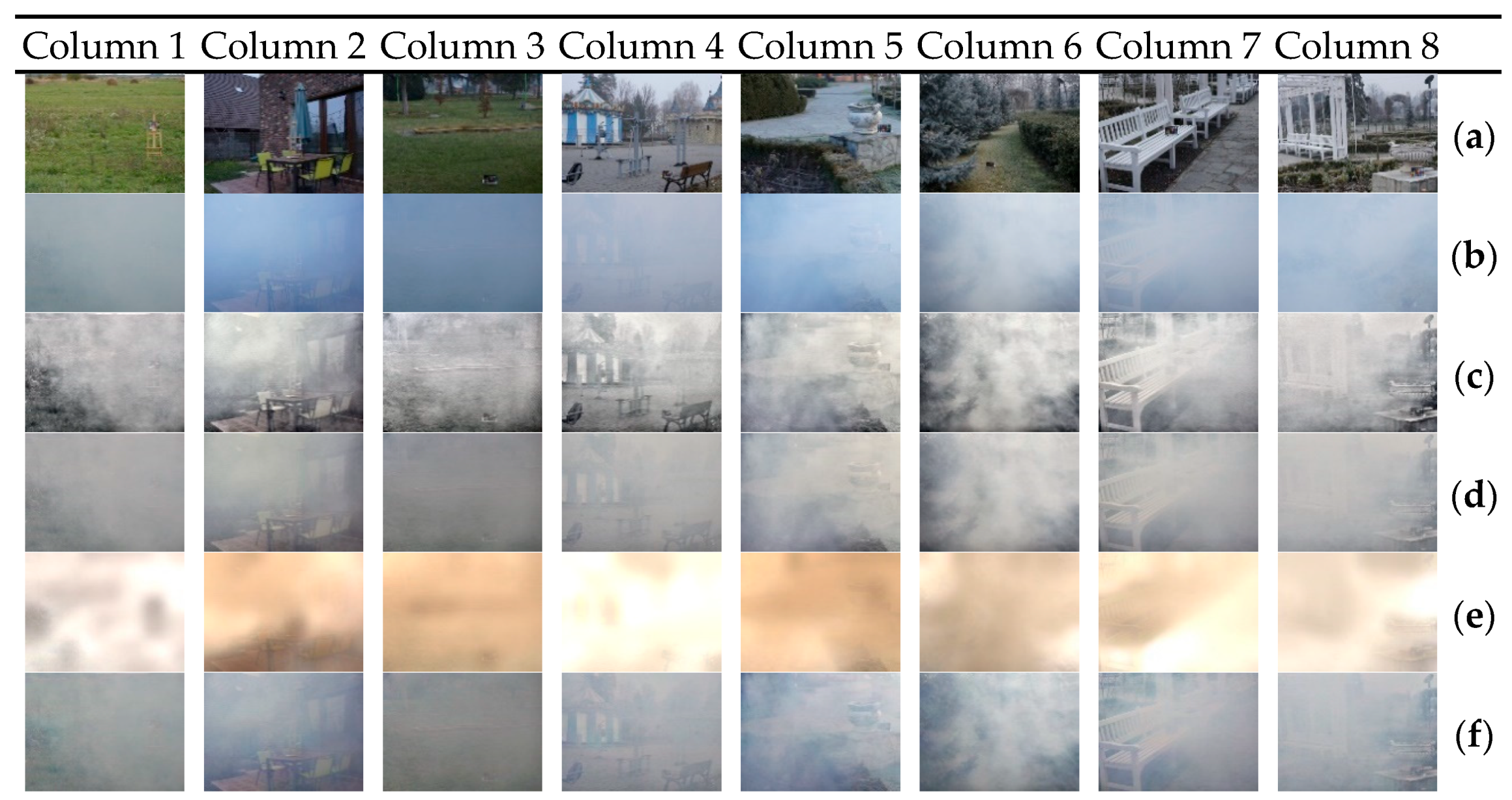
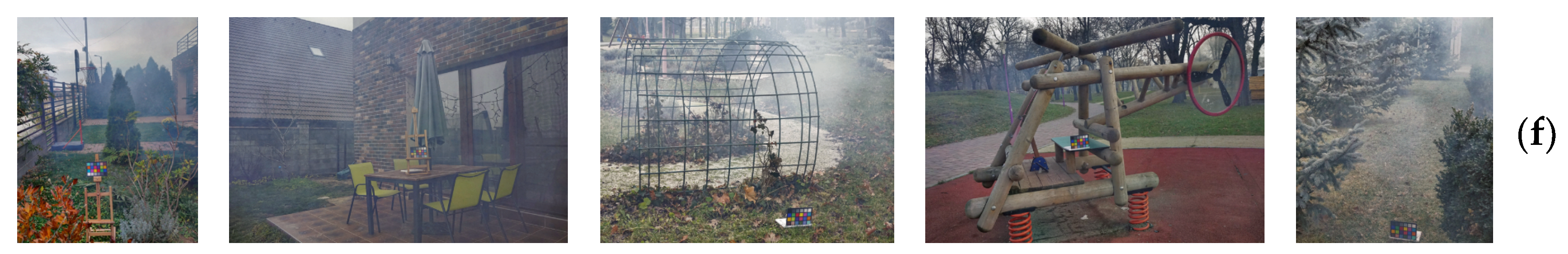
4.1. Visual Comparison of Various Hazy Images

In this study, Laboratory for Image and Video Engineering (LIVE) [34] and sand dust image [35] datasets were used as test images to perform dehazing on actual hazy and color-cast images. Through Figure 8 and Figure 9, the dehazing performance on various color-cast hazy images was evaluated. Figure 8 and Figure 9 show the visual evaluation of the hazy images of various concentrations and hazy images damaged by various colors, respectively.

The visual evaluation in Figure 8 shows that HRDCP resulted in an intensified halo effect, shadowing, and a grayscale effect with increased haze concentration, and in particular, the saturation of the image dropped significantly due to the excessive contrast improvement in the image with a lower-middle concentration. In addition, HRDCP added red color to the sky area due to the white balance in the low image, with an extremely small addition of haze color. NGCCLAHE also added red color to the low image, and reduced saturation in the lower-middle image. In contrast, WSDACC increased color distortion as the yellow haze was distributed widely in the image. The proposed method showed excellent visual results for all images in Figure 8, and in the low image, it showed superb results in both visibility improvement and color restoration. Furthermore, it preserved as much as possible the sky area and lighting area, which are susceptible to distortion, noise, or shadowing.

Figure 8. Color restoration results of hazy images at various concentration levels: (a) original hazy image, (b) HRDCP, (c) NGCCLAHE, (d) WSDACC, and (e) proposed dehazing method.

Figure 9. Color restoration results of hazy images cast with various colors: (a) original hazy image, (b) HRDCP, (c) NGCCLAHE, (d) WSDACC, and (e) proposed dehazing method.

Figure 9 presents the color restoration performance against the red, yellow, green, and blue color-cast images in order, all of which included objects such as trees, rivers, and lakes whose colors are similar to hazy veils. As shown in Figure 9, HRDCP, which offers strong color restoration performance, lost the color information of the scenes in all test images. While NGCCLAHE exhibited a considerable improvement over HRDCP, the loss of color information was considerable in the case of large-scale scenes in the yellow or blue image, such as trees or lakes. WSDACC introduced color distortions for images with high saturation haze veils, similar to that in Figure 9. In contrast, our approach used an airlight color detection algorithm to preserve the original colors of scenes, even those closely resembling haze.

In this study, the results of the general hazy images, in which airlight is in grayscale, are shown in Figure 10, and the versatility of the algorithm was evaluated. To verify the dehazing performance of the distant scenes shown in Figure 10, their detailed shots are shown in Figure 11. The detailed areas correspond to the white squares in Figure 10.

In this paper, quality parameters and no-reference evaluation metrics are used to evaluate the quality of typical fog images. For the resulting image in Figure 10, the edge ratio (e) [36], the mean slope ratio ($\overline{\mathit{r}}$) [36], fog reduction factor (FRF) [37], and perception-based image quality evaluator (PIQE) [38] were used as quality evaluation metrics to show the quantitative results. Of these, the higher the e, $\overline{\mathit{r}}$, FRF, and PIQE, the better the quality, and the lower the PIQE, the better the value. The results of all quality metrics for Figure 10 are shown in Table 1.

Figure 10. Color-restored dehazing results of general hazy images: (a) original hazy image, (b) HRDCP, (c) NGCCLAHE, (d) WSDACC, and (e) proposed dehazing method.

Figure 10 shows images with high saturation or those in which an object occupies a large area of the image. In particular, test images 1~4 biased the histogram of the image with the colors of red vehicles, orange flowers, yellow fields, and green mountains.

Figure 11. Color restoration dehazing results of general hazy images: (a) original hazy image, (b) HRDCP, (c) NGCCLAHE, (d) WSDACC, and (e) proposed dehazing method.

Table 1. Visual quality assessment results for a typical fog image.

	Image	HRDCP	NGCCLAHE	WSDACC	Proposed
e	Test 1	0.0488	0.0738	0.0669	0.1049
	Test 2	0.1016	0.1186	−0.1143	0.1220
	Test 3	0.4725	0.3975	0.0997	0.5101
	Test 4	0.0583	0.0864	−0.0107	0.0723
	Test 5	0.4270	0.3816	0.0155	0.3979
	Average	0.2217	0.2116	0.0114	0.2415
$\overline{r}$	Test 1	2.2533	1.7719	0.4047	1.3618
	Test 2	2.9243	2.1153	1.6180	1.3698
	Test 3	2.2332	1.7682	0.9952	1.5707
	Test 4	2.4951	1.9173	1.0384	1.3632
	Test 5	2.7109	1.9456	0.7972	1.6737
	Average	2.5233	1.9036	0.9707	1.4678
FRF	Test 1	0.3485	0.4788	−0.0226	0.4585
	Test 2	0.0888	0.1256	−0.2988	0.1285
	Test 3	0.0783	0.0237	0.0349	0.1731
	Test 4	0.3383	0.3456	−0.0530	0.3544
	Test 5	0.5303	0.4742	−0.0401	0.5797
	Average	0.2768	0.2896	−0.0759	0.3388
PIQE	Test 1	44.4367	46.4053	50.2147	40.1527
	Test 2	40.0996	35.7676	31.8466	29.2613
	Test 3	43.7708	42.1776	35.8692	40.3450
	Test 4	44.0385	42.1096	42.0236	36.5857
	Test 5	26.1658	30.8974	38.2872	25.0304
	Average	39.7023	39.4715	39.6483	34.2750

Table 1. Visual quality assessment results for a typical fog image.

	Image	HRDCP	NGCCLAHE	WSDACC	Proposed
e	Test 1	0.0488	0.0738	0.0669	0.1049
	Test 2	0.1016	0.1186	−0.1143	0.1220
	Test 3	0.4725	0.3975	0.0997	0.5101
	Test 4	0.0583	0.0864	−0.0107	0.0723
	Test 5	0.4270	0.3816	0.0155	0.3979
	Average	0.2217	0.2116	0.0114	0.2415
$\overline{r}$	Test 1	2.2533	1.7719	0.4047	1.3618
	Test 2	2.9243	2.1153	1.6180	1.3698
	Test 3	2.2332	1.7682	0.9952	1.5707
	Test 4	2.4951	1.9173	1.0384	1.3632
	Test 5	2.7109	1.9456	0.7972	1.6737
	Average	2.5233	1.9036	0.9707	1.4678
FRF	Test 1	0.3485	0.4788	−0.0226	0.4585
	Test 2	0.0888	0.1256	−0.2988	0.1285
	Test 3	0.0783	0.0237	0.0349	0.1731
	Test 4	0.3383	0.3456	−0.0530	0.3544
	Test 5	0.5303	0.4742	−0.0401	0.5797
	Average	0.2768	0.2896	−0.0759	0.3388
PIQE	Test 1	44.4367	46.4053	50.2147	40.1527
	Test 2	40.0996	35.7676	31.8466	29.2613
	Test 3	43.7708	42.1776	35.8692	40.3450
	Test 4	44.0385	42.1096	42.0236	36.5857
	Test 5	26.1658	30.8974	38.2872	25.0304
	Average	39.7023	39.4715	39.6483	34.2750

The detailed shots in Figure 11 show the close scenes in test 1 and the distant scenes in tests 2–6. The assessment of the visibility improvement performance in Figure 11 shows that HRDCP and NGCCLAHE resulted in a bluish haze that is clearly seen in tests 1 and 3, through which poor visibility from the original image could be verified. Further, HRDCP and NGCCLAHE failed to preserve the saturation of the object and scene in all tests, except in test 5, and as such, the distant scenes became blurry. The detailed shot in test 5, which showed a low saturation level, also resulted in poor visibility with HRDCP and NGCCLAHE compared to the proposed method. WSDACC showed considerably insufficient visibility in distant scenes, similar to Figure 10, due to the dark background color and poor dehazing performance. The proposed method preserved the hue of the distance scenes in all detailed shots and showed superb visibility improvement. The proposed method showed the most natural and highest contrast.

The results in Table 1 show that the proposed method exhibited lower values for $\overline{\mathit{r}}$, which represents the contrast between the background and the object, compared to HRDCP and NGCCLAHE. However, visually, it produced the sharpest images in the results, as shown in Figure 10 and Figure 11, and had the best visual quality for e, FRF, and PIQE, with the exception of $\overline{\mathit{r}}$. In particular, the proposed method showed remarkably high results in the fog concentration difference FRF and quality score PIQE, indicating strong defogging performance.

4.2. Performance Evaluation Using Ground Truth Image

This study used PSNR, CIEDE2000 [39], and CIE94 [40] as evaluation indexes for the assessment of dehazing performance and color restoration performance. PSNR evaluates the quality of images, and CIEDE2000 and CIE94 calculate color differences between the original and restored images to evaluate the tone of the images. For comparison, we presented the scores of CIEDE2000 and CIE94 from the average and the square root of the average on the CIEDE2000 and CIE94 maps, respectively. In this context, higher PSNR scores indicate better performance, while lower CIEDE2000 and CIE94 scores indicate superior performance.

Unfortunately, no actual haze dataset with biased colors for an objective assessment index has been proposed for open source. Thus, we used Dense-HAZE [41], a popular dataset that offers actual hazy images, as our input images. The Dense-HAZE dataset provides real hazy and ground truth images using specialized fog-generating machines on haze-free scenes as input images. In particular, Dense-HAZE generated a bluish haze in all images, even though there was no added color because the fog machine produced dark-colored fog. Thus, we used Dense-HAZE to evaluate both the visibility and color restoration performance in color-biased hazy images. The Dense-HAZE images used and the results from each algorithm are shown in Figure 12, and the quantitative evaluation results from Figure 12 are presented in Table 2.

Dense-HAZE images in Figure 12 had limitations for visual comparison due to the dense haze, compared with the images shown in Figure 11. However, the results from HRDCP and NGCCLAHE showed that the images resulted in considerable performance in the edges due to high dehazing performance, and due to strong contrast and white balance, the overall images showed gray tone. In addition, WSDACC added a strong red color, opposite to the blue haze, resulting in a new color cast in the output images. In contrast, our method increased the visibility of the hazy areas and preserved the object color, similar to that of the ground truth image. Our results, in particular, accurately recognized the original object colors and, similar to NGCCLAHE’s results, naturally removed haze in some areas.

The quantitative comparison of the restored images from Dense-HAZE in Table 2 showed the best results for the proposed method, while in the existing methods, NGCCLAHE showed superior results both in PSNR and CIEDE2000, as well as CIE94, and HRDCP showed high performance almost similar to the method proposed in PSNR in some areas. However, the proposed method showed a particularly considerable deviation in CIEDE2000 and CIE94 compared with the existing methods, including HRDCP, demonstrating color restoration performance closer to the original.

Figure 12. Comparison of the resulting images of the Dense-HAZE dataset: (a) ground truth image; (b) hazy image; (c) HRDCP; (d) NGCCLAHE; (e) WSDACC; (f) proposed dehazing method.

Table 2. Comparison of PSNR, CIEDE2000, and CIE94 of the Dense-HAZE dataset.

	Image	HRDCP	NGCCLAHE	WSDACC	Proposed
PSNR	Column 1	25.6801	27.6232	12.9887	29.3583
	Column 2	18.3533	20.6083	13.9061	21.9567
	Column 3	18.5879	24.1812	14.3154	25.4478
	Column 4	30.8870	30.2614	13.8340	31.8312
	Column 5	18.8900	19.9033	15.2217	21.8796
	Column 6	17.9036	16.6909	13.6151	18.6536
	Column 7	21.8741	22.5892	12.3425	23.5417
	Column 8	23.6716	23.1715	14.6542	24.4558
	Average	21.9810	23.1286	13.8597	24.6406
CIEDE 2000	Column 1	65.0429	58.3551	68.994	55.5198
	Column 2	80.8358	83.0109	101.178	70.1804
	Column 3	71.6801	64.0757	83.9369	59.0298
	Column 4	62.8703	60.0154	102.421	44.4957
	Column 5	87.177	86.2875	86.9605	67.5862
	Column 6	73.3669	74.9258	88.2843	71.7223
	Column 7	67.9032	70.0154	97.6982	57.9881
	Column 8	73.1579	75.1231	84.7146	62.4879
	Average	72.75426	71.47611	89.27344	61.12628
CIE94	Column 1	40.996	37.9644	61.1512	35.6449
	Column 2	56.8746	54.1844	64.2783	51.4884
	Column 3	55.6438	47.5759	64.1364	46.0510
	Column 4	38.7339	39.17	62.4296	37.1594
	Column 5	55.4124	53.6296	59.5817	43.9504
	Column 6	57.1691	57.7260	64.5412	54.5976
	Column 7	50.4363	47.0993	64.8543	45.4348
	Column 8	46.5830	45.4304	59.5978	43.7097
	Average	50.2311	47.8475	62.5713	44.7545

Table 2. Comparison of PSNR, CIEDE2000, and CIE94 of the Dense-HAZE dataset.

	Image	HRDCP	NGCCLAHE	WSDACC	Proposed
PSNR	Column 1	25.6801	27.6232	12.9887	29.3583
	Column 2	18.3533	20.6083	13.9061	21.9567
	Column 3	18.5879	24.1812	14.3154	25.4478
	Column 4	30.8870	30.2614	13.8340	31.8312
	Column 5	18.8900	19.9033	15.2217	21.8796
	Column 6	17.9036	16.6909	13.6151	18.6536
	Column 7	21.8741	22.5892	12.3425	23.5417
	Column 8	23.6716	23.1715	14.6542	24.4558
	Average	21.9810	23.1286	13.8597	24.6406
CIEDE 2000	Column 1	65.0429	58.3551	68.994	55.5198
	Column 2	80.8358	83.0109	101.178	70.1804
	Column 3	71.6801	64.0757	83.9369	59.0298
	Column 4	62.8703	60.0154	102.421	44.4957
	Column 5	87.177	86.2875	86.9605	67.5862
	Column 6	73.3669	74.9258	88.2843	71.7223
	Column 7	67.9032	70.0154	97.6982	57.9881
	Column 8	73.1579	75.1231	84.7146	62.4879
	Average	72.75426	71.47611	89.27344	61.12628
CIE94	Column 1	40.996	37.9644	61.1512	35.6449
	Column 2	56.8746	54.1844	64.2783	51.4884
	Column 3	55.6438	47.5759	64.1364	46.0510
	Column 4	38.7339	39.17	62.4296	37.1594
	Column 5	55.4124	53.6296	59.5817	43.9504
	Column 6	57.1691	57.7260	64.5412	54.5976
	Column 7	50.4363	47.0993	64.8543	45.4348
	Column 8	46.5830	45.4304	59.5978	43.7097
	Average	50.2311	47.8475	62.5713	44.7545

Because the very thick haze in each image of Figure 12 made visual confirmation difficult, the O-HAZE [42] dataset was used for visual and quantitative evaluations of the ground truth images. While O-HAZE offered actual hazy images in the same way as Dense-HAZE, the spreading of haze in normal concentration allowed for a visual comparison and the determination of the effect of the color restoration algorithm on general hazy images. The results of the visual comparison of O-HAZE in this study are shown in Figure 13, and the quantitative results are shown in Table 3.

This paper compares the processing time of HRDCP, NGCCLAHE, and WSDACC with the proposed method, using O-HAZE and Dense-HAZE datasets. The input images for the experiments are the fog images in Figure 12 and Figure 13, and the respective processing times are shown in Table 4.

Figure 13. Comparison of the resulting images from O-HAZE dataset (a) ground truth image; (b) hazy image; (c) HRDCP; (d) NGCCLAHE; (e) WSDACC; (f) proposed dehazing method.

The results of the visual comparison of the O-HAZE images showed that the hazy images in Figure 13 had general gray-tone haze as opposed to those of Dense-HAZE; thus, the existing color restoration methods damaged the color information of objects to some degree, as discussed in Section 4.1. When compared to the ground truth images, the resulting HRDCP and NGCCLAHE images showed clear color distortion of the objects, and in particular, the hue became excessively brighter than in the original images. Further, HRDCP applied excessive contrast improvement on Figure 13, resulting in large shadows on the images, and compared to the original images, the edges of close objects were severely emphasized. Furthermore, WSDACC increased the red color in some hazy images, resulting in color cast. In contrast, our method increased the visibility of hazy areas, preserving the object color close to that of the ground truth images. In particular, our results preserved the object color and increased the contrast of the areas where haze existed, producing natural results without visual burdens.

Table 3. Comparison of PSNR, CIEDE2000, and CIE94 of the O-HAZE dataset.

	Image	HRDCP	NGCCLAHE	WSDACC	Proposed
PSNR	Column 1	25.4914	34.3623	25.8197	39.6625
	Column 2	29.1756	35.6395	15.9377	43.3597
	Column 3	26.6413	32.1664	26.1565	35.7555
	Column 4	28.0609	39.7892	41.5410	55.1319
	Column 5	24.4291	33.0331	14.5984	39.0183
	Average	26.7597	34.9981	24.8107	42.5856
CIEDE 2000	Column 1	65.7187	57.9394	74.5331	49.2308
	Column 2	57.8792	53.9991	104.156	32.3133
	Column 3	56.3077	56.0603	56.4345	46.6211
	Column 4	65.2795	59.8458	50.2132	38.6987
	Column 5	57.8297	55.5612	85.6416	47.3394
	Average	60.6029	56.6812	74.1957	42.8407
CIE94	Column 1	45.5594	34.8882	44.2823	30.2724
	Column 2	45.5774	38.5965	63.0140	29.9591
	Column 3	43.8257	36.1606	42.5899	31.0338
	Column 4	44.7354	32.1035	32.3704	21.3600
	Column 5	49.3693	38.4082	61.5174	31.1818
	Average	45.8134	36.0314	48.7548	28.7614

Table 3. Comparison of PSNR, CIEDE2000, and CIE94 of the O-HAZE dataset.

	Image	HRDCP	NGCCLAHE	WSDACC	Proposed
PSNR	Column 1	25.4914	34.3623	25.8197	39.6625
	Column 2	29.1756	35.6395	15.9377	43.3597
	Column 3	26.6413	32.1664	26.1565	35.7555
	Column 4	28.0609	39.7892	41.5410	55.1319
	Column 5	24.4291	33.0331	14.5984	39.0183
	Average	26.7597	34.9981	24.8107	42.5856
CIEDE 2000	Column 1	65.7187	57.9394	74.5331	49.2308
	Column 2	57.8792	53.9991	104.156	32.3133
	Column 3	56.3077	56.0603	56.4345	46.6211
	Column 4	65.2795	59.8458	50.2132	38.6987
	Column 5	57.8297	55.5612	85.6416	47.3394
	Average	60.6029	56.6812	74.1957	42.8407
CIE94	Column 1	45.5594	34.8882	44.2823	30.2724
	Column 2	45.5774	38.5965	63.0140	29.9591
	Column 3	43.8257	36.1606	42.5899	31.0338
	Column 4	44.7354	32.1035	32.3704	21.3600
	Column 5	49.3693	38.4082	61.5174	31.1818
	Average	45.8134	36.0314	48.7548	28.7614

Table 4. Comparison of execution time (sec) between O-HAZE and Dense-HAZE.

	Image	HRDCP	NGCCLAHE	WSDACC	Proposed
Dense-HAZE	Column 1	0.1627	$4.20\times {10}^{-6}$	3.5735	0.3697
	Column 2	0.2981	$4.20\times {10}^{-6}$	7.1377	0.7203
	Column 3	0.4315	$5.40\times {10}^{-6}$	10.7535	1.0884
	Column 4	0.5636	$4.50\times {10}^{-6}$	14.5247	1.4456
	Column 5	0.7025	$5.30\times {10}^{-6}$	18.1768	1.8046
	Average	0.4317	$\mathbf{4.72} \times {10}^{-6}$	10.8332	1.0857
O-HAZE	Column 1	0.1963	$3.80\times {10}^{-6}$	4.5718	0.4331
	Column 2	0.3885	$4.50\times {10}^{-6}$	9.0356	0.8792
	Column 3	0.6069	$3.70\times {10}^{-6}$	13.4543	1.3217
	Column 4	0.8094	$3.10\times {10}^{-6}$	17.9645	1.7932
	Column 5	1.0060	$4.20\times {10}^{-6}$	22.4588	2.2431
	Column 6	1.1899	$5.00\times {10}^{-6}$	27.0179	2.6768
	Column 7	1.3723	$4.10\times {10}^{-6}$	31.4922	3.1199
	Column 8	1.5712	$4.10\times {10}^{-6}$	36.0234	3.5757
	Average	0.8926	$\mathbf{4.06} \times {10}^{-6}$	20.2523	2.0053

Table 4. Comparison of execution time (sec) between O-HAZE and Dense-HAZE.

	Image	HRDCP	NGCCLAHE	WSDACC	Proposed
Dense-HAZE	Column 1	0.1627	$4.20\times {10}^{-6}$	3.5735	0.3697
	Column 2	0.2981	$4.20\times {10}^{-6}$	7.1377	0.7203
	Column 3	0.4315	$5.40\times {10}^{-6}$	10.7535	1.0884
	Column 4	0.5636	$4.50\times {10}^{-6}$	14.5247	1.4456
	Column 5	0.7025	$5.30\times {10}^{-6}$	18.1768	1.8046
	Average	0.4317	$\mathbf{4.72} \times {10}^{-6}$	10.8332	1.0857
O-HAZE	Column 1	0.1963	$3.80\times {10}^{-6}$	4.5718	0.4331
	Column 2	0.3885	$4.50\times {10}^{-6}$	9.0356	0.8792
	Column 3	0.6069	$3.70\times {10}^{-6}$	13.4543	1.3217
	Column 4	0.8094	$3.10\times {10}^{-6}$	17.9645	1.7932
	Column 5	1.0060	$4.20\times {10}^{-6}$	22.4588	2.2431
	Column 6	1.1899	$5.00\times {10}^{-6}$	27.0179	2.6768
	Column 7	1.3723	$4.10\times {10}^{-6}$	31.4922	3.1199
	Column 8	1.5712	$4.10\times {10}^{-6}$	36.0234	3.5757
	Average	0.8926	$\mathbf{4.06} \times {10}^{-6}$	20.2523	2.0053

The quantitative comparison of the restoration images of O-HAZE in Table 3, similar to Table 2, showed that our proposed method showed the best results. Our proposed method demonstrated greater deviations from Dense-HAZE compared to existing methods and achieved superior visibility improvement and color restoration performance values.

The results in Table 4 show that the proposed algorithm has a faster execution time than WSDACC, but it took longer than NGCCLAHE and WSDACC due to the computational process of clustering.

4.3. Limitations and Discussion of the Proposed Approach

Dehazing can be used for a wide range of image types [15,16,17,18,19,20,21,22]. However, since this paper uses clustering to perform dehazing, color distortion occurs in some images where airglow cannot be extracted, such as underwater images and low-light images.

In addition, the proposed method uses fixed parameter values output by the dataset to run an algorithm that preserves the sense of space and color of the original image. Thus, extremely distant scenes may show lower visibility compared to closer objects, as shown in the results in Figure 10 and Figure 13.

Finally, the computational speed of the proposed method is somewhat slower than the existing method, as shown in Table 4. To improve the limitations of the proposed method, we will study how to solve the saturation weighting and complex computation process.

5. Conclusions

This paper proposes an approach based on the saturation of airglow in the LAB channel to restore color in color-cast fog images. The proposed method uses the CIELAB color space for both color correction and dehazing to address the problem of color distortion in traditional RGB channels. The proposed method first white-balances only the hue of the airglow or sky area, and not the entire scene, reflecting the nature of the fog which is directly affected. To detect the saturation of the airglow, the dominant color output method is used to cluster the LAB images, and the classified clusters are assigned an area score to select the optimal airglow area. In addition, the a and b channels of the airglow are white-balanced by running a modified gray world hypothesis in LAB.

To dehaze the color-restored fog image, a weighted depth map is computed by analyzing the correlation between brightness, saturation, and the depth of the fog. To solve the problem of traditional dehazing where objects in the close-range view are darkened when visibility is increased, we divide the image based on the mean of L, so that different distances are weighted differently. To address shading and noise in the sky area, we also take advantage of the fact that the restored airglow is achromatic to separate distant objects from the airglow. The parameters of the depth map are estimated using multiple linear regression based on their linear nature, and the final output depth map is applied to the atmospheric scattering model to run dehazing.

The quantitative and visual analysis results of the existing method and the proposed method demonstrate that the proposed method addresses the problems of existing color restoration dehazing methods, such as scenes with fog and objects with similar saturation and scenes with widespread highly saturated objects, and shows superior color restoration performance. In terms of dehazing, the proposed method preserves objects in the close-range view that are less affected by fog while improving the visibility of the distant view, thus preserving the information in the original image as much as possible. It also handles distant objects separately from airglow, while also addressing shading, noise, etc., in the airglow area due to severe visibility enhancement.

References

- He, K.; Sun, J.; Tang, X. Single image haze removal using dark channel prior. IEEE Trans. Pattern Anal. Mach. Intell. 2011, 33, 2341–2353. [Google Scholar]
- Tarel, J.P.; Hauti, N. Fast visibility restoration from a single color or gray level image. In Proceedings of the IEEE International Conference on Computer Vision, Kyoto, Japan, 29 September–2 October 2009; pp. 2201–2208. [Google Scholar]
- He, K.; Sun, J.; Tang, X. Guided image filtering. IEEE Trans. Pattern Anal. Mach. Intell. 2013, 35, 1397–1409. [Google Scholar] [CrossRef]
- Li, Z.; Zheng, J.; Zhu, Z.; Yao, W.; Wu, S. Weighted guided image filtering. IEEE Trans. Image Process. 2015, 24, 120–129. [Google Scholar]
- Zhu, Q.; Mai, J.; Shao, L. A fast single image haze removal algorithm using color attenuation prior. IEEE Trans. Image Process. 2015, 24, 3522–3533. [Google Scholar]
- Gao, Y.; Hu, H.M.; Li, B.; Guo, Q.; Pu, S. Detail preserved single image dehazing algorithm based on airlight refinement. IEEE Trans. Multimed. 2019, 21, 351–362. [Google Scholar] [CrossRef]
- Berman, D.; Treibitz, T.; Avidan, S. Single image dehazing using haze-lines. IEEE Trans. Pattern Anal. Mach. Intell. 2020, 42, 720–734. [Google Scholar] [CrossRef]
- Lee, S.M.; Kang, B.S. A 4K-capable hardware accelerator of haze removal algorithm using haze-relevant features. J. Inf. Commun. Converg. Eng. 2022, 20, 212–218. [Google Scholar] [CrossRef]
- Cheon, B.W.; Kim, N.H. A modified steering kernel filter for AWGN removal based on kernel similarity. J. Inf. Commun. Converg. Eng. 2022, 20, 195–203. [Google Scholar] [CrossRef]
- Huang, S.C.; Chen, B.H.; Wang, W.J. Visibility restoration of single hazy images captured in real-world weather conditions. IEEE Trans. Circuits Syst. Video Technol. 2014, 24, 1814–1824. [Google Scholar] [CrossRef]
- Dhara, S.K.; Roy, M.; Sen, D.; Biswas, P.K. Color cast dependent image dehazing via adaptive airlight refinement and non-linear color balancing. IEEE Trans. Circuits Syst. Video Technol. 2021, 31, 2076–2081. [Google Scholar] [CrossRef]
- Peng, Y.T.; Lu, Z.; Cheng, F.C.; Zheng, Y.; Huang, S.C. Image haze removal using airlight white correction, local light filter, and aerial perspective prior. IEEE Trans. Circuits Syst. Video Technol. 2020, 30, 1385–1395. [Google Scholar] [CrossRef]
- Harald, K. Theorie der Horizontalen Sichtweite: Kontrast und Sichtweite; Keim and Nemnich: Munich, Germany, 1924; Volume 12, pp. 33–53. [Google Scholar]
- Narasimhan, S.G.; Nayar, S.K. Vision and the atmosphere. Int. J. Comput. Vis. 2002, 48, 233–254. [Google Scholar] [CrossRef]
- Zhou, J.; Zhang, D.; Ren, W.; Zhang, W. Auto color correction of underwater images utilizing depth information. IEEE Geosci. Remote Sens. Lett. 2022, 19, 1504805. [Google Scholar] [CrossRef]
- Wang, K.; Shen, L.; Lin, Y.; Li, M.; Zhao, Q. Joint iterative color correction and dehazing for underwater image enhancement. IEEE Robot. Autom. Lett. 2021, 6, 5121–5128. [Google Scholar] [CrossRef]
- Li, H.; Zhuang, P.; Wei, W.; Li, J. Underwater image enhancement based on dehazing and color correction. In Proceedings of the IEEE International Conference on Parallel & Distributed Processing with Applications, Big Data & Cloud Computing, Sustainable Computing & Communications, Social Computing & Networking, Xiamen, China, 16–18 December 2019; pp. 1365–1370. [Google Scholar]
- Li, C.Y.; Guo, J.C.; Cong, R.M.; Pang, Y.W.; Wang, B. Underwater image enhancement by dehazing with minimum information loss and histogram distribution prior. IEEE Trans. Image Process. 2016, 25, 5664–5677. [Google Scholar] [CrossRef]
- Gao, G.; Lai, H.; Jia, Z.; Liu, Y.; Wang, Y. Sand-dust image restoration based on reversing the blue channel prior. IEEE Photonics J. 2020, 12, 2. [Google Scholar] [CrossRef]
- Shi, Z.; Feng, Y.; Zhao, M.; Zhang, E.; He, L. Let you see in sand dust weather: A method based on halo-reduced dark channel prior dehazing for sand-dust image enhancement. IEEE Access 2019, 7, 116722–116733. [Google Scholar] [CrossRef]
- Shi, Z.; Feng, Y.; Zhao, M.; Zhang, E.; He, L. Normalised gamma transformation-based contrast-limited adaptive histogram equalisation with colour correction for sand–dust image enhancement. IET Image Process. 2020, 14, 747–756. [Google Scholar] [CrossRef]
- Ding, X.; Wang, Y.; Fu, X. An image dehazing approach with adaptive color constancy for poor visible conditions. IEEE Geosci. Remote Sens. Lett. 2022, 19, 6504105. [Google Scholar] [CrossRef]
- Zuiderveld, K.J. Contrast limited adaptive histogram equalization. In Graphics Gems, 4th ed.; Academic Press Professional, Inc.: Cambridge, MA, USA, 1994; pp. 474–485. [Google Scholar]
- Gautam, S.; Gandhi, T.K.; Panigrahi, B.K. An improved air-light estimation scheme for single haze images using color constancy prior. IEEE Signal Process. Lett. 2020, 27, 1695–1699. [Google Scholar] [CrossRef]
- Lam, E.Y. Combining gray world and retinex theory for automatic white balance in digital photography. In Proceedings of the Ninth International Symposium on Consumer Electronics, Macau, China, 14–16 June 2005; pp. 134–139. [Google Scholar]
- Provenzi, E.; Gatta, C.; Fierro, M.; Rizzi, A. A spatially variant white-patch and gray-world method for color image enhancement driven by local contrast. IEEE Trans. Pattern Anal. Mach. Intell. 2008, 30, 1757–1770. [Google Scholar] [CrossRef]
- Chang, H.; Fried, O.; Liu, Y.; DiVerdi, S.; Finkelstein, A. Palette-based photo recoloring. ACM Trans. Graph. 2015, 34, 139. [Google Scholar] [CrossRef]
- Akimoto, N.; Zhu, H.; Jin, Y.; Aoki, Y. Fast soft color segmentation. In Proceedings of the IEEE/CVF Conference on Computer Vision and Pattern Recognition, Seattle, WA, USA, 13–19 June 2020; pp. 8277–8286. [Google Scholar]
- Chang, Y.; Mukai, N. Color feature based dominant color extraction. IEEE Access 2022, 10, 93055–93061. [Google Scholar] [CrossRef]
- Kim, J.H.; Jang, W.D.; Sim, J.Y.; Kim, C.S. Optimized contrast enhancement for real-time image and video dehazing. J. Vis. Commun. Image Represent. 2013, 24, 410–425. [Google Scholar] [CrossRef]
- Liu, L.; Cheng, G.; Zhu, J. Improved single haze removal algorithm based on color attenuation prior. In Proceedings of the IEEE 2nd International Conference on Information Technology, Big Data and Artificial Intelligence, Chongqing, China, 17–19 December 2021; pp. 1166–1170. [Google Scholar]
- Wu, Q.; Ren, W.; Cao, X. Learning interleaved cascade of shrinkage fields for joint image dehazing and denoising. IEEE Trans. Image Process. 2020, 29, 1788–1801. [Google Scholar] [CrossRef]
- Ancuti, C.; Ancuti, C.O.; De Vleeschouwer, C. D-HAZY: A dataset to evaluate quantitatively dehazing algorithms. In Proceedings of the IEEE International Conference on Image Processing, Phoenix, AZ, USA, 25–28 September 2016; pp. 2226–2230. [Google Scholar]
- Choi, L.K.; You, J.; Bovik, A.C. Referenceless perceptual image defogging. In Proceedings of the Southwest Symposium on Image Analysis and Interpretation, San Diego, CA, USA, 6–8 April 2014; pp. 165–168. [Google Scholar]
- IEEE Dataport. Sand Dust Image Data. 2020. Available online: https://ieee-dataport.org/documents/sand-dust-image-data (accessed on 19 September 2023).
- Hautière, N.; Tarel, J.P.; Aubert, D.; Dumont, É. Blind contrast enhancement assessment by gradient ratioing at visible edges. Image Anal. Stereol. 2011, 27, 87–95. [Google Scholar] [CrossRef]
- Kansal, I.; Kasana, S.S. Improved color attenuation prior based image de-fogging technique. Multimed. Tools Appl. 2020, 79, 12069–12091. [Google Scholar] [CrossRef]
- Venkatanath, N.; Praneeth, D.; Bh, M.C.; Channappayya, S.S.; Medasani, S.S. Blind image quality evaluation using perception based features. In Proceedings of the 2015 Twenty First National Conference on Communications, Mumbai, India, 27 February–1 March 2015; pp. 1–6. [Google Scholar]
- Sharma, G.; Wu, W.; Dalal, E.N. The CIEDE2000 color-difference formula: Implementation notes, supplementary test data, and mathematical observations. Color Res. Appl. 2005, 30, 21–30. [Google Scholar] [CrossRef]
- McDonald, R.; Smith, K.J. CIE94-a new colour-difference formula. J. Soc. Dye Colour 2008, 111, 376–379. [Google Scholar] [CrossRef]
- Ancuti, C.O.; Ancuti, C.; Sbert, M.; Timofte, R. Dense-Haze: A Benchmark for image dehazing with Dense-Haze and haze-free images. In Proceedings of the IEEE International Conference on Image Processing, Taipei, Taiwan, 22–25 September 2019; pp. 1014–1018. [Google Scholar]
- Ancuti, C.O.; Ancuti, C.; Timofte, R.; Vleeschouwer, C.D. O-HAZE: A dehazing benchmark with real hazy and haze-free Outdoor Images. In Proceedings of the IEEE/CVF Conference on Computer Vision and Pattern Recognition Workshops, Salt Lake City, UT, USA, 18–22 June 2018; pp. 867–875. [Google Scholar]
Disclaimer/Publisher’s Note: The statements, opinions and data contained in all publications are solely those of the individual author(s) and contributor(s) and not of MDPI and/or the editor(s). MDPI and/or the editor(s) disclaim responsibility for any injury to people or property resulting from any ideas, methods, instructions or products referred to in the content. |
© 2023 by the authors. Licensee MDPI, Basel, Switzerland. This article is an open access article distributed under the terms and conditions of the Creative Commons Attribution (CC BY) license (https://creativecommons.org/licenses/by/4.0/).