Research on the Identification of Bridge Structural Damage Using Variational Mode Decomposition and Convolutional Self-Attention Neural Networks

Abstract

Convolutional neural networks (CNN) are widely used for structural damage identification. However, the presence of environmental disturbances introduces noise into the acquired acceleration response data, impairing the performance of CNN models. In this study, we apply empirical mode decomposition (EMD) and variational mode decomposition (VMD) to denoise the data from a steel truss bridge. By comparing the smoothness and convergence of the obtained modal functions (IMFs) using EMD and VMD, we confirm the effectiveness of VMD in smoothing and denoising the bridge structure signals. Additionally, we propose a convolutional self-attention neural network (CSANN) model to extract features and identify damage in the denoised data using VMD. Comparative analysis of the CNN, LSTM, and GRU models reveals that the VMD-CSANN model outperforms the others in terms of damage localization and identification accuracy. It also exhibits excellent performance when handling noise-contaminated data with a noise level of 10%. These findings demonstrate the efficacy of the proposed method for identifying internal damage in steel truss structures, while maintaining smoothness and robustness during processing.

1. Introduction

In recent years, the establishment of an efficient health monitoring system capable of accurately detecting internal signals from civil structures has emerged as a prominent concern in the field of civil engineering [1,2,3,4]. In the structural health monitoring system (SHMS), classical on-site measurement methods such as ambient vibration testing [5], forced vibration testing [6], and impact vibration testing [7], which are direct methods, often require the installation of numerous sensors directly on the bridge structure [8,9], and the selection of a vibration parameter that is sensitive to structural damage (e.g., frequency [10], mode shape [11], strain energy [12], etc.), the parameter is then extracted using sensors and analyzed using a specific method [13,14]. It is necessary to overcome uncertainties associated with the structural model and the model parameters themselves, including measurement errors, temperature and humidity variations, and other external environmental influences on the structural vibration characteristics. Characteristic signal feedback is utilized to determine the presence of damage in civil structures, enabling the assessment of its location, extent, as well as the current state, functionality, and trend of structural damage [15,16,17,18].

Currently, structural damage identification can be categorized into two main approaches: (a) Local detection of structural damage using techniques such as gamma-ray, ultrasonic, and electromagnetic testing [19]. (b) Global detection of structural damage through frequency response functions (e.g., acceleration response) and modal parameters (e.g., damping, natural frequency, mode shapes), enabling non-destructive detection of existing damage in structures under undamaged or minimally damaged conditions [20,21].

Existing research has demonstrated that methods based on dynamic response signal data yield significantly improved results in structural damage identification compared to traditional non-destructive techniques [22].

Many cutting-edge techniques in computer vision today rely on deep neural networks [23]. The seamless integration of deep learning technology into the realm of civil engineering has prompted both domestic and international researchers to explore the potential of deep learning models like convolutional neural networks (CNN) [24,25,26] and recurrent neural networks (RNN) in addressing challenges within the field of structural damage identification. Sheng [27] employed wavelet transformation on one-dimensional data, subsequently fed into a CNN model as images. This validated the reliability of two-dimensional convolutional neural networks for fault diagnosis. Khodabandehlou et al. [28] utilized acceleration data from a scaled model of a reinforced concrete bridge as experimental data and employed a two-dimensional CNN for damage identification, demonstrating the network’s effectiveness in recognizing minor damage. Lin et al. [29] applied CNN to extract acceleration data generated by a simply supported beam finite element model, achieving robust recognition results under various damage conditions and amidst varying noise levels. Liu et al. [30] combined 1D-CNN with the transfer function, utilizing the transfer function of the structural dynamic response of the ASCE benchmark as input data. Comparative analysis with time series and fast Fourier transform (FFT) data revealed that features derived from the transfer function data were more sensitive to damage. Yang Jianxi et al. [31] introduced a structural damage identification method that integrates CNN and long short-term memory (LSTM). The CNN model was employed to extract topological correlation features from vibration acceleration input data across multiple event windows, while LSTM further captured temporal dimension features. Experimental data from a scale model of a bridge construction were tested and yielding favorable results.

Variational modal decomposition (VMD) stands out as a cutting-edge technique for decomposing nonlinear signals into multiple frequency bands, distinguishing itself from conventional spatial frequency and subspace signal processing methods. Notably, it eliminates the need for computationally intensive calculations for both recursive and non-recursive signals. This breakthrough allows for the comprehensive construction and resolution of variational problems, achieving the separation of signal frequency bands [32,33]. This innovative time–frequency analysis method accomplishes signal decomposition by constructing and solving constrained variational problems. It transforms the original signal into a specified number of intrinsic mode functions (IMFs), a capability that is highly effective in handling nonlinear and non-smooth signals. In the realm of structural damage identification, highly sensitive time series sample parameters are found at critical structural points, categorizable into the time domain, frequency domain, and time–frequency domain based on signal types [34]. Utilizing VMD to preprocess vibration signals from structural damage points, followed by smoothing and noise reduction, proves to be a viable approach. Currently, numerous scholars have delved into the efficacy of VMD in processing vibration signals related to structural damage. Zhang Jian et al. [35] introduced a structural damage identification method leveraging VMD and Chirplet transform, successfully achieving precise location and quantification of structural damage, both in single and multi-point damage scenarios.

Wang Qiuxiao [36] furthered the exploration of VMD’s capabilities by integrating it with deep learning models like CNN, LSTM, and BiLSTM. This integration was tested using the IASC-ASCE SHM benchmark model, yielding impressive accuracy in damage identification. This underscores the promising potential of VMD in the field of structural damage identification.

Self-attention mechanisms represent a variant of attention mechanisms, adept at capturing internal correlations within data or features themselves [37]. The self-attention mechanism facilitates the model in capturing long-range dependencies between different positions within an input sequence. These mechanisms enable the model to comprehend data representation across various locations and subspaces, facilitating the learning of relevant information in different representation subspaces. Consequently, this empowers the model to discern correlations between distinct parts of the entire input information [38]. In time series data, there are correlations between data sequences from the same measurement point at different time steps. However, the efficacy of signal decomposition or feature extraction techniques is often constrained in capturing these correlations. By incorporating the self-attention mechanism, the model can be trained on extensive data to learn the inherent dependencies and assign weighted importance to different values. This application enhances the model’s capability to discern similar response waveform patterns to a certain degree, thereby improving its overall discriminative power.

At the heart of the convolutional self-attention neural network (CSANN) lies the self-attention mechanism layer and the convolutional layer. The self-attention layer is crucial for correlating features at different nodes of the time series data with the model output, thereby determining the representation of the time series. Meanwhile, the convolutional layer focuses on extracting local feature information within the temporal neighborhood, performing essential feature transformations [39].

Drawing inspiration from multivariate decomposition and smoothing processes applied to time series signals through variational mode decomposition in various fields [40,41], this paper introduces a damage identification model that combines VMD and CSANN. This model is then applied to structural damage identification using the acceleration response data from multi-sensor measurement points on a steel truss structure as an example.

In different operating conditions, multiple sets of raw acceleration vibration response signal data were acquired from sensors installed on a steel truss bridge structure. The acquired data was subjected to noise contamination and then decomposed using empirical mode decomposition (EMD) and variational mode decomposition (VMD). Comparative evaluation of the obtained sets of intrinsic mode functions (IMFs) based on time–frequency representations confirmed the data value of the IMF components derived from VMD decomposition. Subsequently, the selected IMFs were concatenated and augmented with the original data. The resulting dataset was then fed into a convolutional neural network (CNN) model with the integration of a self-attention mechanism for feature extraction and damage identification. The model was capable of assessing the extent of damage and performing damage localization.

By conducting a comparative analysis between variational mode decomposition (VMD) and empirical mode decomposition (EMD), we employed the VMD-CSANN model to process signal data containing typical levels of background noise, and subsequent comparison with CNN, LSTM, and GRU models. The study confirms the effectiveness and feasibility of the VMD-CSANN model in the identification of engineering structural damage.

2. Methodology

2.1. Variational Mode Decomposition

Introduced in 2014, variational mode decomposition (VMD) is a non-recursive signal decomposition method [42]. VMD operates by seeking a set of modes and their respective center frequencies from the input signal. Through Hilbert transform, the original signal is decomposed into K modal components of limited bandwidth, denoted as $v_k\left(t\right)$. Each IMF possesses a center frequency represented as ${\omega }_t$. The modal decomposition is subject to two constraints: modal superposition and equivalence to the input signal.

To convert the center band of $v_k\left(t\right)$ to its corresponding baseband, the single-sided spectrum of $v_k\left(t\right)$ is computed and multiplied by $e^{-j^{\omega }kt}$:

$$\left[\left(\delta \left(t\right)+\frac{j}{\pi t}\right)\ast v_k\left(t\right)\right]e^{-j^{\omega }kt}$$

(1)

Then, to calculate the square norm of the demodulation gradient:

$$\left\{\begin{array}{c}\{{min}_{\left\{v_k\right\},\left\{{\omega }_k\right\}}\{{\displaystyle \sum _k}\Vert {\partial }_t[(\delta (t)+\frac{j}{\pi t})\ast v_k(t)]e^{-j^{\omega }kt}\}{\Vert }_2^2\}\\ s.t. {\displaystyle \sum _k}{v}_{k }\left(t\right)=f\left(t\right)\end{array}\right.$$

(2)

In Formula (2), $\left\{v_k\right\}=\left\{v_1,\cdots ,v_k\right\}$ represent the decomposed intrinsic mode function (IMF) components, $\left\{{\omega }_k\right\}=\left\{{\omega }_1,\cdots ,{\omega }_k\right\}$ represent the central frequency of each component, $\delta \left(t\right)$ represents the Dirac delta function, $j$ is the imaginary unit, and $f\left(t\right)$ is the original signal. The unconstrained optimization is achieved by extending the Lagrange expression:

$$\begin{array}{ll}L(\{v_k\},\{{\omega }_k\},\lambda )=& \alpha {\displaystyle \sum _k}||{\partial }_i[(\delta (t)+\frac{j}{\pi t})\ast v_k(t)]e^{-j^{\omega }kt}{\Vert }_2^2+|f(t)\\ & -{\displaystyle \sum _k}{u}_k\left(t\right){\Vert }_2^2+\lambda ((t),f(t)-{\displaystyle \sum _k}{u}_k(t))\end{array}$$

(3)

By employing the alternating direction multiplication operator for the intrinsic modal parameters and IMF central frequency, Equation (4) is utilized to iteratively update ${\hat{u}}_k^{(n+1)}$ until the optimal solution of the function is attained:

$${\hat{u}}_k^{(n+1)} (\omega )=\frac{\hat{f}(\omega )-{\displaystyle {\sum }_{i\ne k}}{\hat{u}}_i(\omega )+\frac{\hat{\lambda }(\omega )}{2}}{1+2\alpha (\omega -{\omega }_k)}$$

(4)

In Equation (4), ${\mathsf{\omega }}_k^{(n+1)}$ is iteratively updated by Equation (5):

$${\mathsf{\omega }}_k^{(n+1)} (\omega )=\frac{{\int }_0^{\mathrm{\infty }}\omega |{\hat{u}}_k (\omega ){|}^{2}dw}{{\int }_0^{\mathrm{\infty }}|{\hat{u}}_k (\omega ){|}^{2}du}$$

(5)

${\lambda }^{n+1}$ is updated iteratively according to Equation (6):

$${\lambda }^{n+1}={\lambda }^n+\tau (f-\sum u_k^{n+1})$$

(6)

By iteratively applying the cyclic Equations (2)–(5) until the convergence condition expressed in Equation (7) is met, the optimal decomposition of the original signal $f(t)$ is accomplished:

$${\displaystyle \sum _k}\Vert u_k^{n+1}-u_k^n|{|}_2^2/\Vert u_k^n\Vert <2$$

(7)

2.2. Convolutional Self-Attention Neural Network (CSANN) Model Construction

The CNN model used for target-specific damage identification requires the collection of structural vibration data from the target in order to construct a comprehensive deep learning dataset. In practical engineering applications, a combination of finite element analysis and field testing allows us to acquire the original acceleration responses from each measurement point under different damage states, forming the initial dataset. Furthermore, there exists a correlation between data points at key nodes within the structure, occurring simultaneously. Therefore, segments of acceleration signals within the same time interval are continuously concatenated to enhance the model’s ability to distinguish signals under diverse operating conditions.

During the acquisition process, each signal sample in the dataset is labeled and differentiated using serial number labels based on the state of the structure. Once the dataset is appropriately labeled, it serves as the training set to be fed into the CNN network. The core structure of the CNN model comprises an input layer, a hidden layer, and an output layer. Typically, the hidden layer is composed of several convolution layers, pooling layers, and fully connected layers, as illustrated in Figure 1.

In this paper, we employ a one-dimensional convolutional neural network to construct our model. When compared to two-dimensional convolutional neural networks, the one-dimensional variant offers the advantages of being lighter in weight and easier to train due to having fewer parameters. Moreover, it demonstrates superior performance when processing time series data. Importantly, 1D-CNN typically does not require altering the dimension of the input signal, allowing it to preserve the signal characteristics to the fullest extent.

Drawing inspiration from the earlier work of scholar Krizhevsky [43], we adopt the rectified linear unit (ReLU) as the activation function for the convolutional layer. This choice effectively enhances the performance of the deep convolutional neural network when compared to alternative functions like sigmoid and tanh. In our paper, ReLU is specifically chosen as the activation function for constructing the convolutional neural network model for function $K$, expressed as follows:

$$K=F_{ReLU}(x)=max(0,x)$$

(8)

In Equation (8), $F_{ReLU}(x)$ represents the activation function and $x$ is the element value of the input function. The convolutional layer calculation is shown in Figure 2.

Building upon the foundation of the CNN model, we incorporate a self-attention layer. The attention mechanism can be elucidated through the mapping relationships between the query vector, a series of key-value vector pairs, and the resulting output vectors. The core formula of the self-attention mechanism is presented in Equation (9). In this context, the output vector is derived from a weighted summation of the value vectors. Each value vector’s weighting coefficient is determined by assessing the compatibility between the query vector and its corresponding key vector. The proportion between the query vector and the main vector is then calculated using these weighting coefficients. When the query vector, key vector, and value vector pertain to the same sequence, this is referred to as self-attention.

In the process of computing a series of query vectors, it is customary to combine the query vector, key vector, and value vector. This is achieved by utilizing query matrices, key matrices, and value matrices to enhance computational efficiency. The underlying principle of the self-attention mechanism is depicted in Figure 3. The dot product method involves multiplying two vectors with different matrices, denoted as $w$, to obtain $q$ and $k$. The dot product of $q$ and $k$ yields $\alpha$. In Figure 3, the green portion represents input vectors $a1$ and $a2$, while the gray matrices $W^q$ and $W^k$ represent weight matrices that need to be learned and updated by the model. By multiplying $a1$ with $W^q$, a vector $q$ is obtained, and by multiplying $a2$ with $W^k$, a scalar value $k$ is obtained. Finally, the dot product of $q$ and $k$ yields α, which represents the degree of correlation between the two vectors. On the right side of Figure 3, the additive model mechanism involves multiplying the input vector with the weight matrix, adding them together, projecting the result onto a new function space using $tanh$, and then multiplying it with another weight matrix to obtain the final result. Each α can be calculated, where $q$ is referred to as the query and $k$ as the key.

2.3. VMD-CSANN Joint Model Construction

The $N$ segments of raw acceleration signal time series obtained from different measurement points by sensor devices can be represented as an $N\ast T$ dimensional matrix $M$. The length of this time series is determined by the sampling time and frequency. Each segment of the time series $S_i$ is variational mode decomposition into $K$ intrinsic mode function (IMF) components $v_k\left(t\right)$ using the measurement point as a reference. Based on the decomposed central frequency ${\omega }_t$, the IMF components are recombined to form new local signal sequences $S_t$. These new signal sequences are concatenated with the original signal sequences, using time as a reference, to create feature signals $S_{i,t}$. The combination of all feature signal sequences forms a new feature matrix $M_t$.

After each vector matrix data is preprocessed as input data, it is input into CSANN. The convolution layer extracts the signal features of the data through the convolution operation of the input data, as shown in Figure 4.

The convolution layer begins by initializing $N$ 1-dimensional convolution kernels of length $x$, employing Gaussian functions for random mobilization. These convolution kernels then slide horizontally along the input one-dimensional data matrix with a defined sliding interval. At each position, a product operation and summation is performed on the element values, resulting in a value. Ultimately, the m × 1-dimensional one-dimensional data matrix is transformed into a [(m − x)/k + 1] × n-dimensional output matrix, denoted as $S$.

During the linear operation of data replication, it is customary to perform activation calculations on the output matrix $S$. This entails coupling each element with an active element in the matrix $S$, thereby introducing nonlinear factors. The resulting matrix is then transferred to the next convolution layer for further processing, as follows:

$$f\left(i\right)=s\left(i\right)\times K$$

(9)

In Equation (9), $f\left(i\right)$ represents each data value in the output matrix S after the addition of factors, $s\left(i\right)$ represents each data value in matrix $S$, and $K$ represents the activation function utilized by the convolutional layer.

In the construction of the convolutional neural network model, it is customary to insert pooling layers between adjacent convolutional layers to mitigate overfitting. These pooling layers typically include MaxPooling and AveragePooling. For this study, we employed one-dimensional maximum pooling to process the time series data from the convolution operation, denoted as time series $A$. $A$ was segmented into several informational fragments $A_i$, from which the maximum element value was extracted to form a new input matrix, denoted as $B$:

$$a_{i,max}=\mathrm{m}\mathrm{a}\mathrm{x}\{a_1,a_2,\cdots ,a_i\}$$

(10)

In Formula (10), $a_{i,max}$ are the data obtained after maximum pooling of $a_i$ from the original sequence $A$.

3. Case Study

3.1. Numerical Modeling Construction

Taking the damage identification of a steel truss structure as an example, the real picture of the steel truss structure is shown in Figure 5 and the basic structure is shown in Figure 6.

In this study, we examine how various forms of damage affect the truss structure under different operational conditions. The structural elements are connected using a coupling method, with one end featuring a fixed hinge and the other a sliding hinge connection. The total length of the structure is 8.4 m, with an inner steel pipe diameter of 12 mm and an outer diameter of 18 mm. To simulate real-world conditions in numerical simulations, the four endpoints at the two ends of the steel truss are anchored on four 150 kg pillars. The properties of the steel pipes are detailed in

Table 1. Steel pipe material properties.

Steel Tube Type	Density	Modulus of Elasticity	Poisson’s Ratio	Cross-Sectional Area	Moment of Inertia
Φ18 × 3	7850 kg/m3	2.06 × 1011 Pa	0.3	0.93 cm2	0.414 cm4

.

Modal parameters of the structure are determined through hammering excitation, allowing for an examination of how damage impacts these parameters. Additionally, acceleration signals are collected at each node, and the structural damage response data is derived through the application of transfer functions. This comprehensive approach enables a thorough investigation into the effects of different types of damage on the entire truss structure.

3.2. Preprocessing

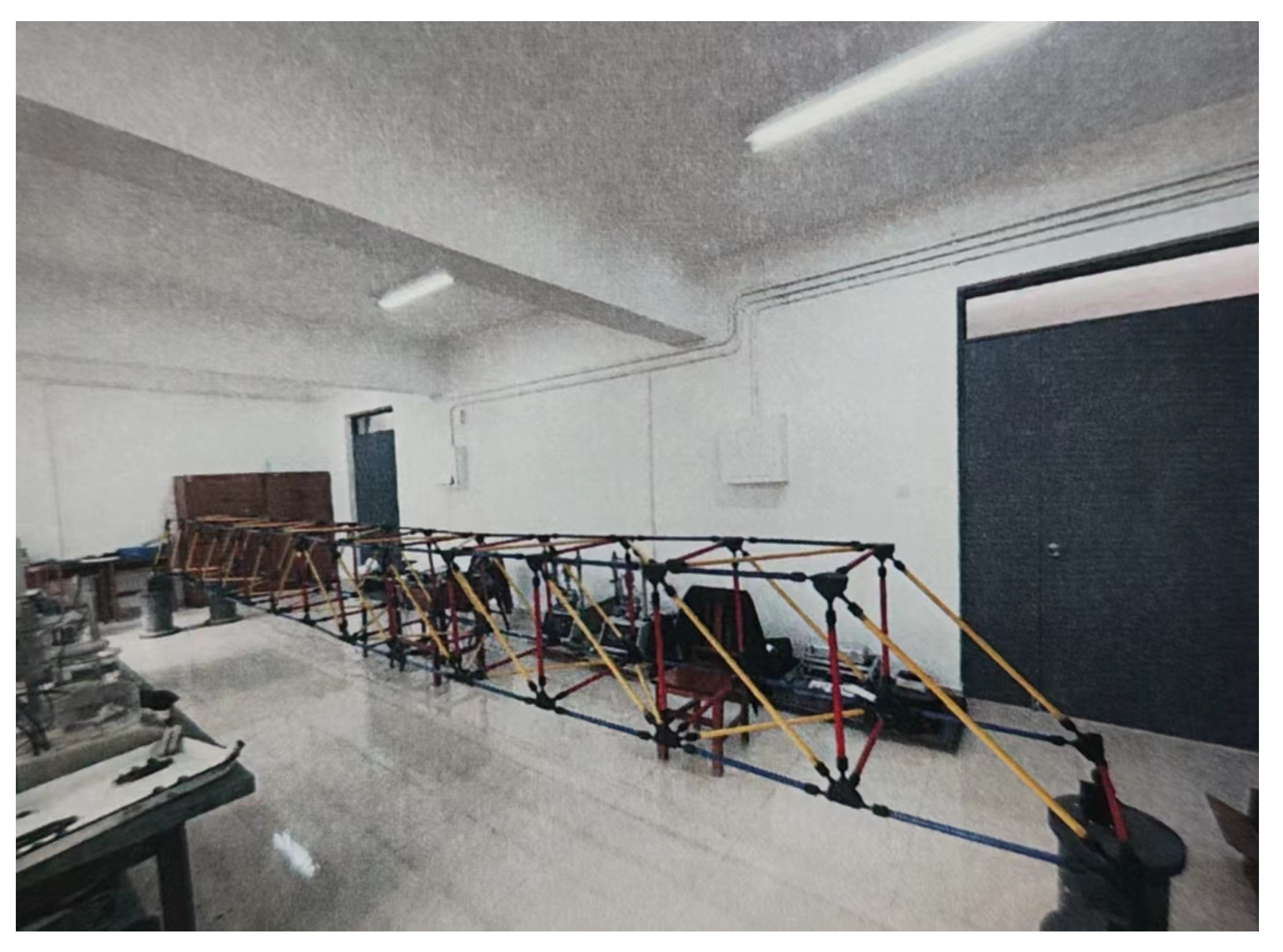
The number of rods in the experimental model is divided into 160 units, and the units are numbered. The sizes of chord, vertical, and belly rods are 0.4 m and 0.65 m, and are divided into 11 working conditions. Damage was created in units 7, 10, and 35. In this experiment, the cutting length is positively correlated with the damage degree. The longer the cutting length is, the lower the stiffness of the rod, and the greater the degree of damage. The cutting length is 10 cm and 20 cm, respectively, and the setting of experimental conditions is shown in

Table 2. Setting table of experimental conditions. The meaning of the + signal indicating the location where the damage occurs.

Working Condition	Damage Unit				Cutting Length
	No. 7	No. 7 Straight Belly Rod	No. 10	No. 35	10 cm	20 cm
WC0	+				+
WC1	+					+
WC2			+		+
WC3			+			+
WC4		+				+
WC5	+		+		+	+
WC6	+		+			+
WC7	+		+		No. 10	No. 10
WC8	+	+	+		No. 10	No. 7 straight belly rod
WC9	+	+				+
WC10	+	+	+		No. 10	No. 7, No. 35

.

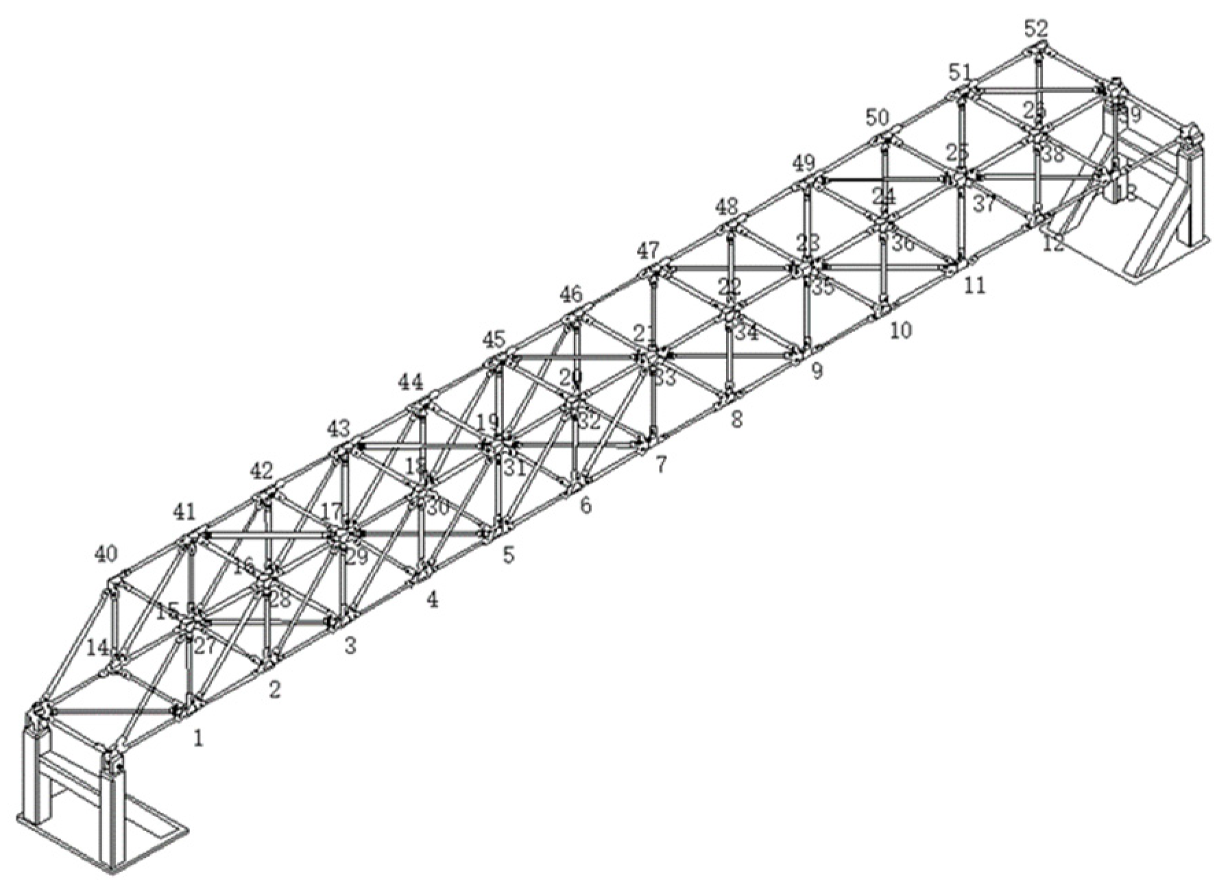
The steel truss structure model has a total of 56 nodes, as shown in the figure. Because the two ends of the model adopt simple support constraints, no sensors are arranged at the two ends of the model, and sensors are only arranged for the remaining 52 nodes, as shown in Figure 7. Due to the limitation of the number of sensors, the modal test is divided into four groups. The acceleration data of each measuring point under pulse excitation were collected with a sampling frequency of 1000 Hz and sampling time of 5 s.

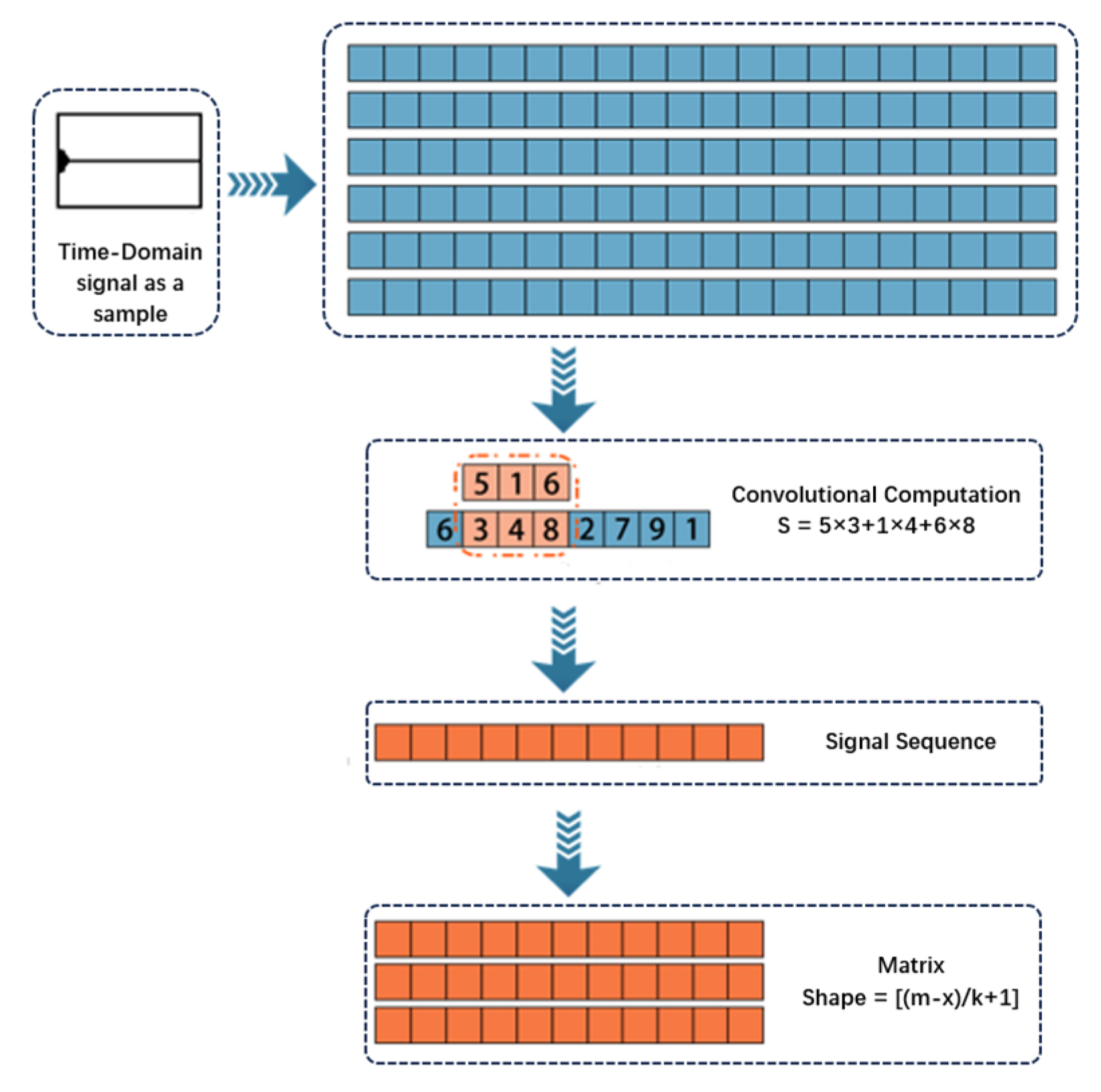
For the single-signal data measured by sensor $N$ at a fixed frequency, since there is a strong correlation between signals at a certain measuring point on the same time scale, the measured acceleration responses at the measuring point within the same time interval are combined with continuous signals, and the signals are integrated into one-dimensional time series data segments. By hammering the center of the bar between different nodes, the damage is caused in different positions of the structure.

The multi-label classification method is used to label the measured data under different damage backgrounds as the label of the working condition, so as to ensure the classification effect of the model is more accurate. By combining the datasets from different operating conditions for all sensor points and their corresponding labels, an original dataset is obtained. The original dataset consists of 11 unprocessed data sets with dimensions of 12,288 × 56, where the operating condition number serves as the label. The 11 original datasets are concatenated, resulting in an intergrated dataset with dimensions of 12,288 × 616. The intergrated dataset is labeled based on the operating condition number. The damaged operating conditions and their corresponding labels are shown in

Table 3. Damage conditions and data labels.

Operating Condition Number	Working Condition	Damage Condition
0	WC0	No. 7 10 cm
1	WC1	No. 7 20 cm
2	WC2	No. 10 10 cm
3	WC3	No. 10 20 cm
4	WC4	No. 7 straight belly rod 20 cm
5	WC5	No. 7 10 cm + No. 10 10 cm
6	WC6	No. 7 20 cm + No. 10 20 cm
7	WC7	No. 7 20 cm + No. 10 10 cm
8	WC8	No. 7 20 cm + No. 7 straight belly rod 20 cm + No. 10 10 cm
9	WC9	No. 7 20 cm + No. 7 straight belly rod 20 cm
10	WC10	No. 7 20 cm + No. 10 10 cm + No. 35 20 cm

.

3.3. Implementation Details

The platform configuration used in this experiment is as follows: platform system—Windows11; hardware configuration—CPU is 11th Gen Intel(R) Core(TM) i7-11800H, memory is 16 G; the graphics card is an NVIDIA GeForce RTX3050Ti 8G*2; experimental framework—Tensorflow2.3.0.

The intergrated dataset was processed using z-score standardization for the preliminary processing of one-dimensional sequence data of each measurement point:

$$z=\frac{x-u}{\sigma }$$

(11)

In Formula (11), $x$ is the single-signal data in the measuring point, $u$ is the mean value of all signal values at the measuring point, and $\sigma$ is the variance of all signal values at the measuring point. Basic attributes such as dimension, quantity and length of data segment do not change after z-score processing, and standardized processing can avoid extreme outliers in the data. The obtained new time series data is defined as a window by the sliding average window, and the sliding window is updated by the fixed sliding window. The sequential average of the window is calculated successively, and the obtained sequential average is connected to generate a new equilong time interval to obtain the dimensionality reduction dataset.

To verify whether the VMD preprocessing step provides positive value to the subsequent neural network, this study first applies noise addition to the aforementioned dimensionality reduction dataset. Gaussian noise with a noise rate of 0.10 $f_n(t)$, resulting in the noisy dataset. The $f_n(t)$ as described in Equation (12).

$$f_n(t)=\cos (4\pi t)+\frac{1}{4}\cos (48\pi t)+\frac{1}{16}\cos (576\pi t)+n$$

(12)

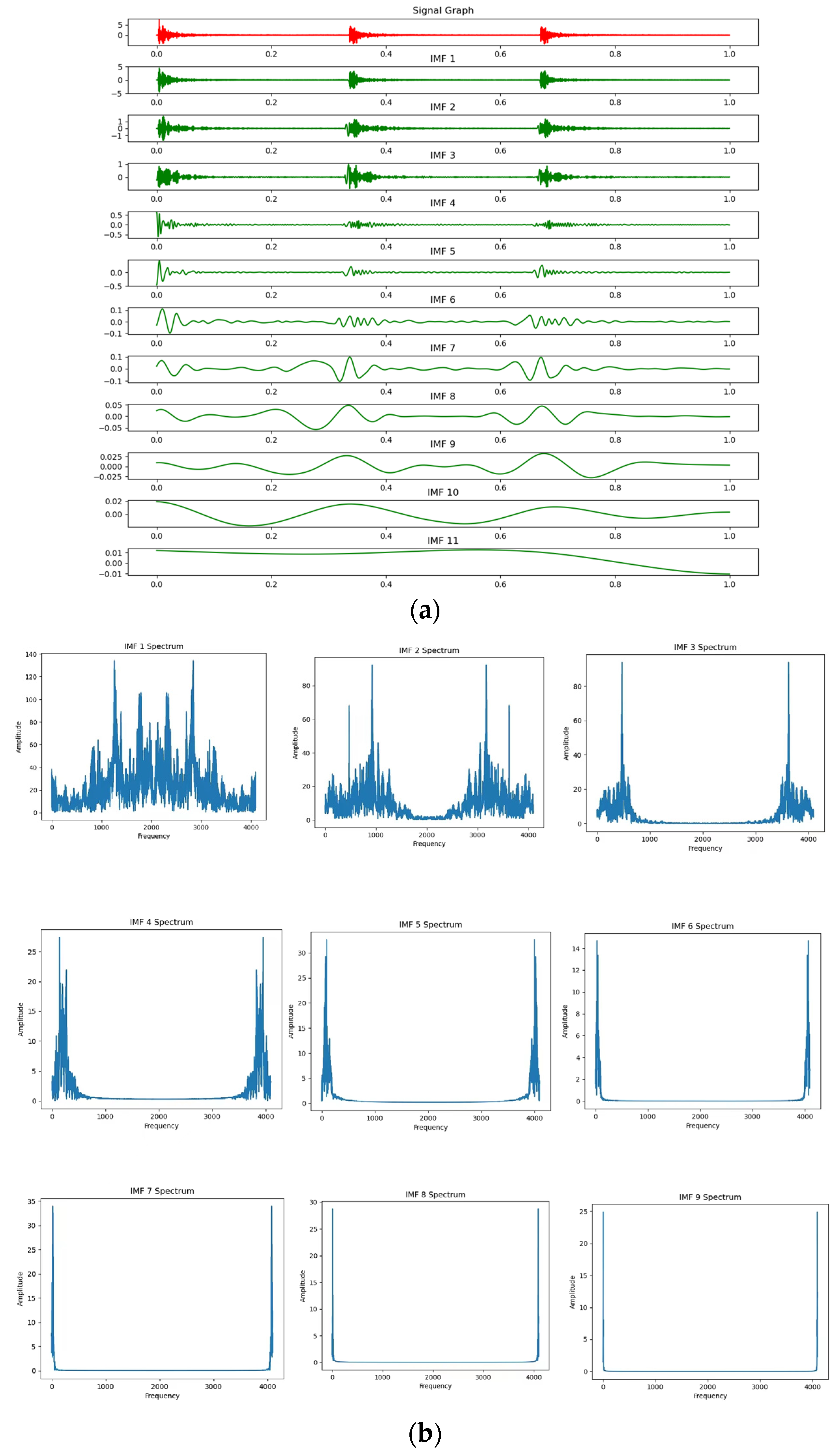
To simulate the interference effects of external environmental factors on the signal data in real-world scenarios, noise is added to the data, and then both EMD and VMD are applied for processing. Figure 8a displays the time-domain waveforms of the original signal and the IMF components obtained after EMD decomposition, while Figure 8b shows the FFT spectra of the IMF components. During the actual experiment, it was observed that the waveforms of the modal components after IMF1 gradually disperse, and the FFT spectra beyond IMF9 become too boundary-dominated, losing their reference value. Therefore, only the FFT spectra of IMF1 to IMF9 are presented.

In the decomposition process of VMD, the Lagrangian multiplier and quadratic penalty play crucial roles as smoothing mechanisms. The Lagrangian multiplier strengthens the constraints, while the quadratic penalty enhances convergence. The Lagrangian multiplier method transforms the constraints into penalty terms in the objective function and adjusts the weight of the penalty term using Lagrangian multipliers. During the hyperparameter tuning process, the regularization strength or weight of the regularization term can be flexibly controlled by setting the penalty factor of VMD, allowing for better control over the smoothness or sparsity of the decomposed mode functions. Additionally, the algorithm’s noise tolerance is set to 0. The mode functions are uniformly initialized, with their initial values set as random numbers from a uniform distribution. The convergence of the algorithm is controlled by setting the tolerance parameter. The decomposition scale is shown in

Table 4. The important hyperparameters related to VMD decomposition.

VMD
Penalty Factor (alpha)	200
Noise Tolerance (tau)	0
Decomposition Scale (K)	4
Direct Current Part (DC)	0 (None)
Uniform Initialization	1
Tolerance	1 × 10−7
Noise Rate	0.10
Time Domain (T)	4096
f_1 Center Frequency	2
f_2 Central Frequency	24
f_3 Central Frequency	128
f_4 Central Frequency	288

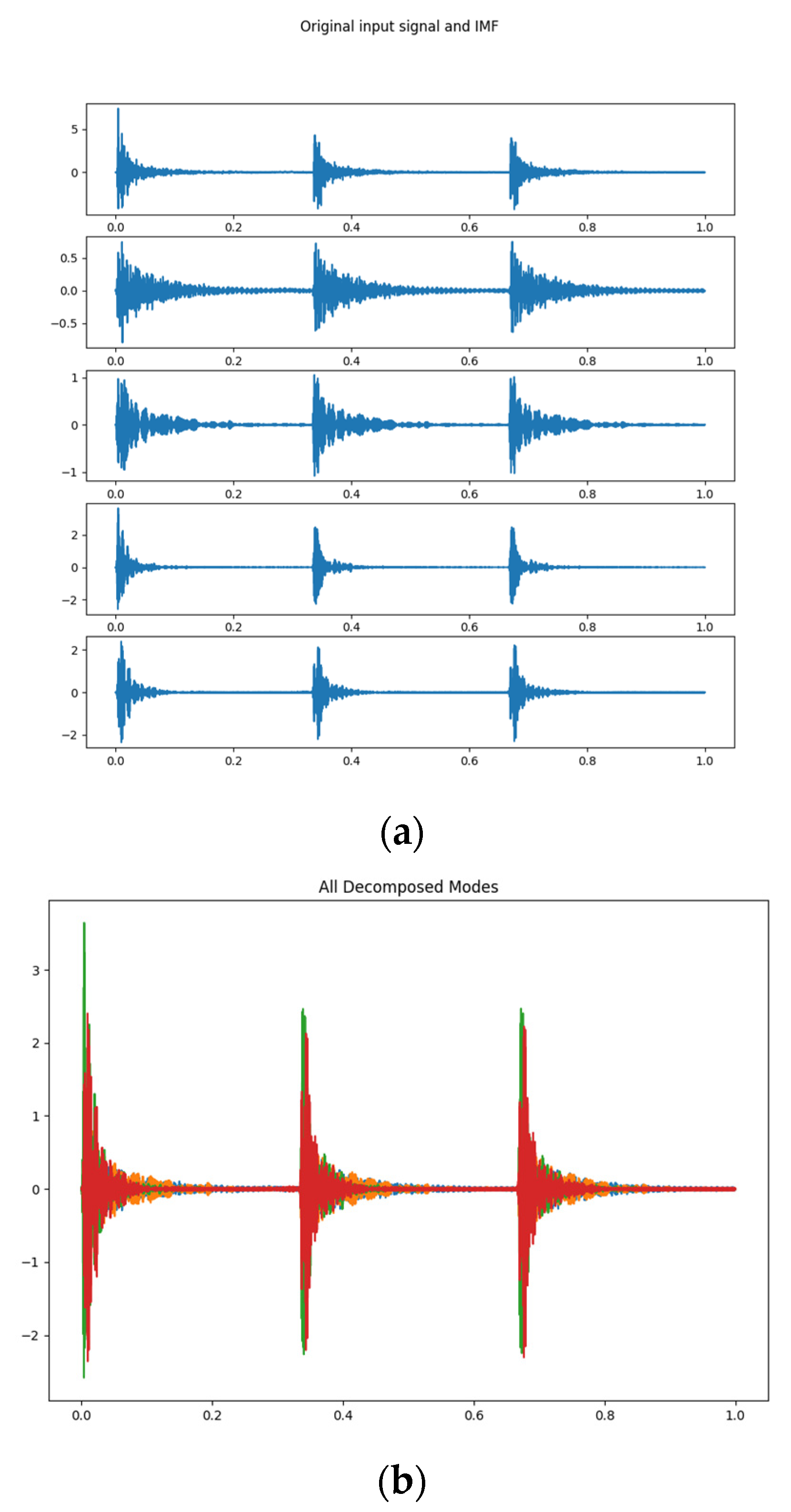
, with the center frequencies of f_1 to f_4 set as 2, 24, 128, and 288, respectively. The core hyperparameters of VMD are listed in Table 4. Figure 9a shows the time-domain waveforms of the original signal and the IMF components obtained after VMD decomposition. Figure 9b displays all the IMF components, Figure 9c shows the FFT spectra of each IMF component.

By comparing the signal representations of intrinsic mode functions (IMFs) obtained through empirical mode decomposition (EMD) and variational mode decomposition (VMD), it is evident that EMD, due to its inability to set the number of decomposed IMFs as hyperparameters, produces multiple signal components that deviate significantly from the original data. In contrast, VMD, with controllable parameters and decomposition guided by the central frequency ${\omega }_t$, yields IMFs that are relatively uniformly dispersed around the original signal.

Additionally, analyzing the FFT spectra of the IMF components obtained from EMD and VMD reveals distinct differences. The FFT spectrum of EMD exhibits gradual marginalization from IMF1 onwards, with IMF10 and IMF11 being severely marginalized, resulting in poor visualization. Therefore, these components are not included in the analysis. In contrast, the FFT spectra of the VMD-decomposed IMFs demonstrate distinct frequency distributions for each IMF component, indicating their potential value for data analysis and experimentation.

Furthermore, in accordance with the theoretical framework outlined in reference [10], this study incorporates Gaussian noise with a 10% noise level into the data, under the prior setting of Lagrangian multipliers and quadratic penalty factors. The purpose is to simulate VMD’s ability to withstand external disturbances and achieve noise robustness under generalized conditions, through its inherent central constraint and non-smooth band decomposition. The resulting decomposition plots clearly indicate that the IMF components generated by VMD do not exhibit sparsity.

It is worth mentioning that in subsequent experimental sections, where VMD decomposition is utilized as input for a neural network model, the final recognition performance further confirms the robustness of VMD’s processing capabilities.

Then, the data set was decomposed by variational mode to obtain the modal component IMF of the data, and the IMF data and noisy dataset were horizontally expanded to obtain the dataset to be trained with dimension 4096 × 1232.

To investigate the impact of acceleration response signal selection criteria on the effectiveness of structural damage identification in this experiment, three experimental schemes were adopted under impact excitation. These schemes involved the selection of three different operating conditions (i.e., extracting data from the dataset with matching labels of the corresponding operating condition number):

(1)

Working conditions WC1, WC3, WC5, WC7, and WC9 are selected;

(2)

Working conditions WC2, 4, 6, 8, and 10 are selected;

(3)

All working conditions are selected.

In different experimental schemes, the quantity of IMF components is determined by the decomposition scale parameter, $k$, in VMD. Leveraging the inherent mode superposition property of VMD, the IMF components can be combined and averaged to accentuate the representation of crucial information, as demonstrated in Equation (13).

$$X(t)={\displaystyle \sum }_{k=1}^K{C}_k(t)$$

(13)

In Equation (13), $X(t)$ represents the original signal, and $C_k(t)$ represents the $k$ mode component.

Through a trial-and-error approach, an evaluation is conducted on each segment obtained by directly concatenating IMF components with the original signal and on the new signal segment obtained by averaging several IMF components and concatenating it with the original signal. Evaluation criteria include assessing whether the IMF signals deviate significantly from the structural resonance characteristics, whether nonlinear breakpoints occur at the concatenation points of the new signal segments, and whether the overall smoothness of the new signal is reduced. After selecting effective components [44] suitable for horizontal concatenation with the original signal, the selected effective components and the new signal data obtained from the original dataset replace the original data. The final selection of effective IMF components related to structural characteristics and the total number of IMF components obtained after VMD decomposition for each of the three schemes are presented in

Table 5. Screening of effective components and the total number of effective components after VMD decomposition of time series signals under the three schemes. The \ symbol indicates that the data has not been applied in this Option.

	Option	Option 1	Option 2	Option 3
Working Condition
WC0		\	\	1/4
WC1		2/4	\	1/4
WC2		\	1/4	2/4
WC3		2/4	\	1/4
WC4		\	2/4	1/4
WC5		2/4	\	2/4
WC6		1/4	2/4	1/4
WC7		2/4	\	2/4
WC8		\	1/4	1/4
WC9		1/4	\	1/4
WC10		\	2/4	2/4

.

The VMD-CSANN model in this paper consists of two sets of hyperparameters. The first set pertains to the parameters that need to be adjusted for VMD decomposition, as described in Table 4. The second set pertains to the hyperparameters that need to be adjusted for the CSANN model, such as the convolution layer size, dropout layer ratio, learning rate, etc. The hyperparameters of the two parts have influence on the final recognition effect of the experiment. There are many methods available for network parameter optimization. In this paper, grid search is used to combine key parameters in the model, take the average accuracy of the final verification set as the objective function, and make multiple comparison adjustments to optimize parameters. Finally, the CSANN model is established by parameter combination as shown in

Table 6. The important hyperparameters related to the CASNN model.

CSANN
Input Shape	4096 × 1
Number of Convolutional Layers	2
Convolution Layer Shape	(16,16) × 1; (64,4) × 1
Number of Pooling Layer	2
Pooling Layer Shape	(2,2) × 2
Learning Rate	0.0002
Batch Size	64
Epoch	50
Number of Cross Verification Folds	5
Number of Self-Attention Layer	1
Self-Attention Layer Count Times	3

.

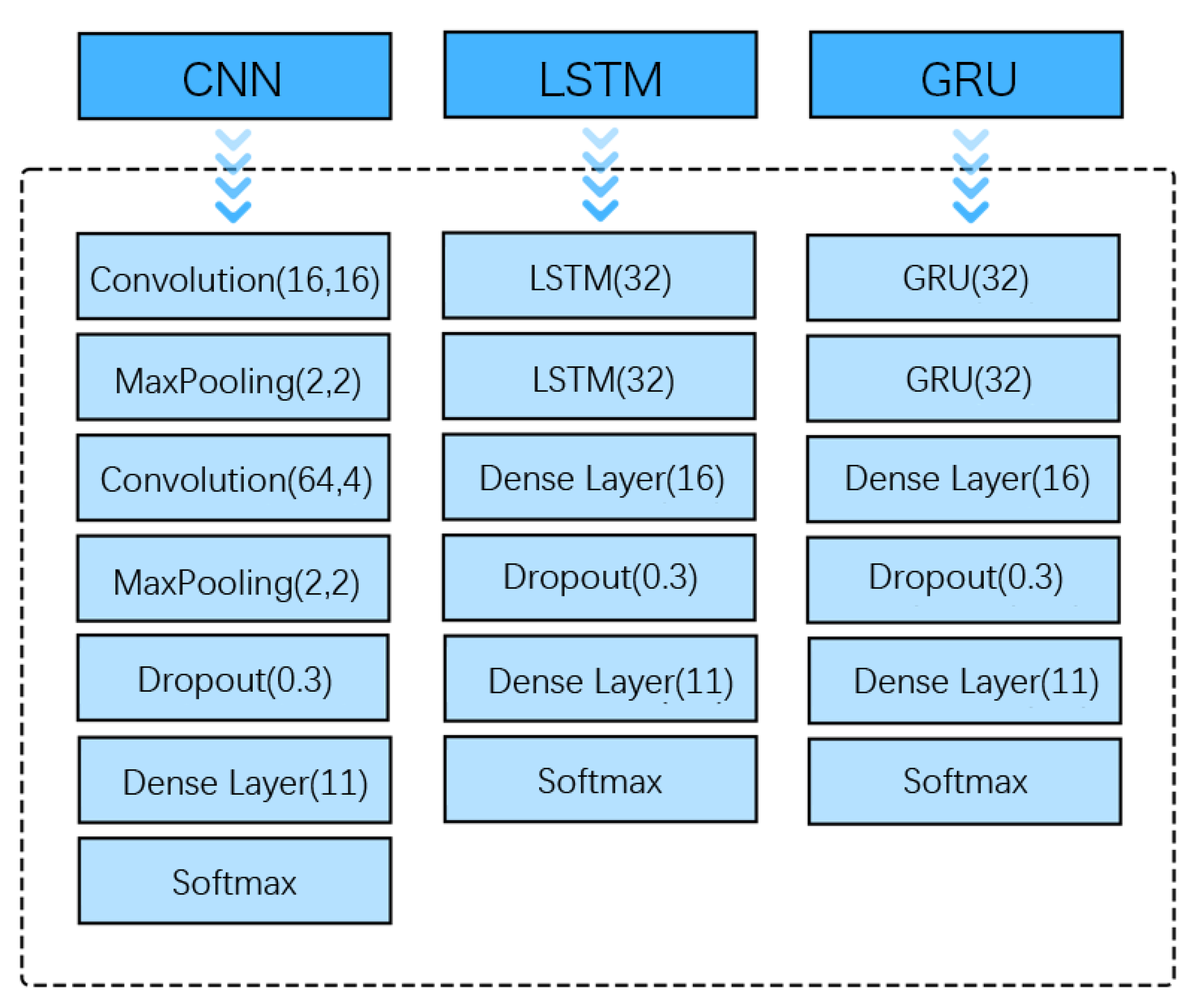
Through comparison experiments between VMD-CSANN and the iconic CNN, LSTM, and GRU models, the effect of the VMD-CSANN model is verified. The comparison neural network models are shown in Figure 10.

3.4. Results

In this paper, the structural damage identification experiment can be regarded as a multi-label classification of multivariate time series. The reference criteria for evaluating the model effect are accuracy of validation set, loss value, F1 score, precision and recall. The accuracy rate is the average of the K validation sets obtained by K-fold cross-validation value and variance, F1 score, accuracy rate, and recall rate are the mean of the K validation sets obtained by K-fold cross-validation, The loss function adopts the cross entropy loss function. For the three experimental schemes, the comprehensive recognition accuracy and loss values of each comparison model were compared horizontally, as shown in

Table 7. Accuracy and loss of each model verification set.

Compared Model	WC1, 3, 5, 7, 9			WC2, 4, 6, 8, 10			All
	Accuracy Rate (Average)	Precision Rate (Variance)	Loss	Accuracy Rate (Average)	Precision Rate (Variance)	Loss	Accuracy Rate (Average)	Precision Rate (Variance)	Loss
CNN	91.87%	94.48%	0.1315	91.87%	94.48%	0.4865	87.80%	89.77%	0.4865
LSTM	77.24%	83.76%	0.7594	80.36%	87.32%	0.6194	88.62%	90.74%	0.3504
GRU	78.86%	79.87%	0.6716	84.82%	86.43%	0.5141	90.24%	91.88%	0.3157
VMD-CSANN	95.12%	93.99%	0.1291	93.75%	94.46%	0.1993	93.90%	94.00%	0.3014

. F-1 value, accuracy rate and recall rate are shown in

Table 8. F1 score, accuracy rate and recall rate of each model validation set.

Compared Model	WC1, 3, 5, 7, 9			WC2, 4, 6, 8, 10			All
	F1 Score (Average)	Precision Rate (Average)	Recall Rate (Average)	F1 Score (Average)	Precision Rate (Average)	Recall Rate (Average)	F1 Score (Average)	Precision Rate (Average)	Recall Rate (Average)
CNN	0.9284	0.9321	0.9306	0.9310	0.9281	0.9218	0.8791	0.8842	0.8769
LSTM	0.7815	0.7865	0.7892	0.8231	0.8219	0.8291	0.8814	0.8852	0.8783
GRU	0.7882	0.7931	0.7872	0.8452	0.8523	0.8493	0.9051	0.9101	0.9089
VMD-CSANN	0.9412	0.9459	0.9482	0.9381	0.9421	0.9401	0.9317	0.9391	0.9401

. The running time of each comparison model is shown in

Table 9. Statistics of running time of each model.

Compared Model	WC1, 3, 5, 7, 9	WC2, 4, 6, 8, 10	All
	Running Time	Running Time	Running Time
CNN	19.5 s	19.7 s	37.4 s
LSTM	16.4 s	16.2 s	32.3 s
GRU	15.8 s	15.1 s	33.1 s
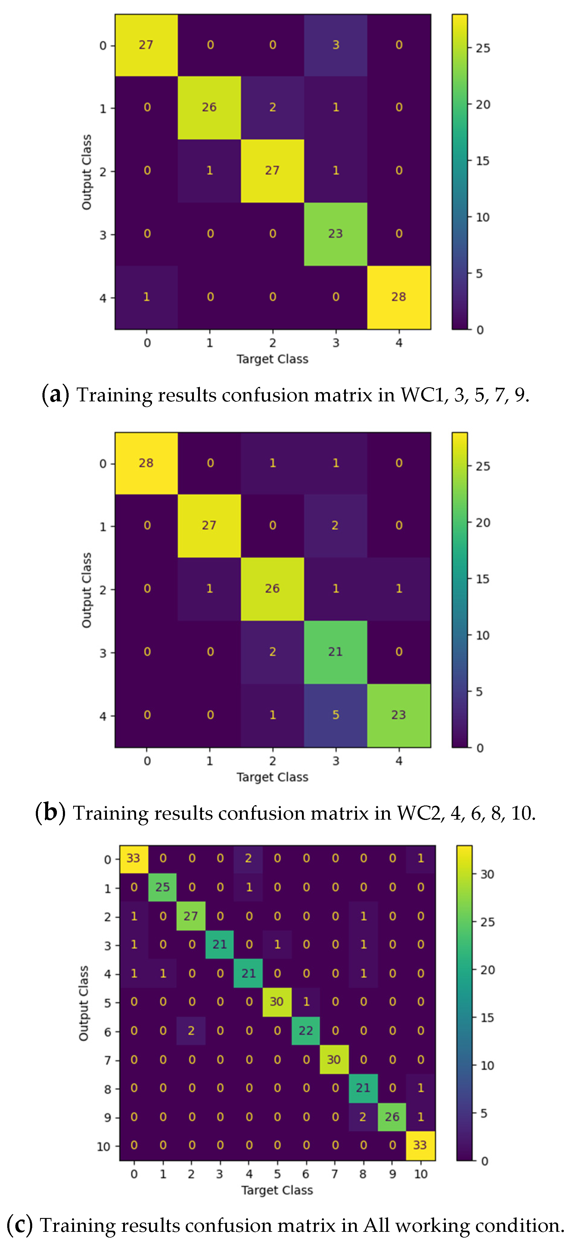
VMD-CSANN	15.4 s	14.9 s	31.8 s

. The confusion matrix generated by the three experimental schemes is shown in Figure 11.

Under the condition of keeping the hyperparameters such as epoch and learning rate consistent among all the compared models, the VMD-CSANN combined model demonstrates superior performance in terms of accuracy, loss value, F1 score, precision, and recall metrics compared to other models. This is attributed to the ability of variational mode decomposition to decompose the original signal, including noisy and non-smooth segments, into several relatively smooth segments. This substantiates that augmenting the VMD-CSANN model with both VMD and self-attention mechanisms leads to improved recognition capabilities, whether for specific working conditions or across the board.

However, it is worth noting that the recognition effectiveness for all working conditions, particularly those with larger datasets, is marginally less optimal compared to specific working conditions. This nuanced difference underscores the importance of considering the specific characteristics and complexities of the data when evaluating model performance.

4. Conclusions

In this paper, we present a structural damage identification method that leverages variational mode decomposition (VMD) in tandem with a convolutional neural network (CSANN). Through numerical simulation experiments involving the acceleration response of steel truss structures, we have observed that, even without employing GPU acceleration, the combined VMD-CSANN model demonstrates superior performance compared to the comparison model. The loss value is also generally lower compared to the comparison models. The total time required for five cross-validations is 36.8 s, slightly faster than the CNN model, yet slower than the LSTM and GRU models.

The correlation value of the VMD-CSANN model surpasses that of the comparison model, indicating superior recognition accuracy and noise resistance. This suggests that the model meets the demands of structural health monitoring system tasks for damage identification. However, it is important to note that this paper primarily focuses on damage pattern recognition within simulated structures. The challenge of recognizing damage in complex engineering structures with real-world signal data warrants further investigation. Additionally, given the more intricate data processing involved in the VMD-CSANN model compared to traditional models, the combination and selection of model structures and hyperparameters are currently constrained. Future research should explore more effective methods for model optimization.

References

1. Zong, Z.H.; Zhong, R.M.; Zheng, P.J.; Qin, Z.Y.; Liu, Q.Q. Damage and safety prognosis of bridge structures based on structural health monitoring: Progress and challenges. Highw. Transp. 2014, 27, 46–57. [Google Scholar]
2. Wang, S.Q.; Xu, M.Q. Modal strain energy-based structural damage identification: A review and comparative study. Struct. Eng. Int. 2019, 29, 234–248. [Google Scholar] [CrossRef]
3. Xu, B.T.; Zhang, X.Z.; Jiang, J.F.; Liu, K.; Wang, S.; Fan, X.J.; Jiang, F.; Li, Y.Q.; Chu, Y.; Liu, T.G. Method of damage location determination based on a neural network using a single fiber Bragg grating sensor. Appl. Opt. 2019, 58, 7251–7257. [Google Scholar] [CrossRef] [PubMed]
4. Deng, F.; Tao, X.; Wei, P.; Wei, S.A. Robust Deep Learning-Based Damage Identification Approach for SHM Considering Missing Data. Appl. Sci. 2023, 13, 5421. [Google Scholar] [CrossRef]
5. Farrat, C.R.; James, G.H., III. System identification from ambient vibration measurements on a bridge. J. Sound Vib. 1997, 205, 1–18. [Google Scholar] [CrossRef]
6. Reiterer, M. Experimentelle und numerische Untersuchung einer bestehenden Eisenbahnbrücke bei Zugüberfahrt. Bautechnik 2020, 97, 473–489. [Google Scholar] [CrossRef]
7. Huang, C.S.; Yang, Y.B.; Lu, L.Y.; Chen, C.H. Dynamic testing and system identification of a multi-span highway bridge. Earthq. Eng. Struct. Dyn. 1999, 28, 857–878. [Google Scholar] [CrossRef]
8. Reiterer, M.; Bettinelli, L.; Schellander, J.; Stollwitzer, A.; Fink, J. Application of Vehicle-Based Indirect Structural Health Monitoring Method to Railway Bridges—Simulation and In Situ Test. Appl. Sci. 2023, 13, 10928. [Google Scholar] [CrossRef]
9. Yamamoto, K.; Shin, R.; Mudahemuka, E. Numerical Verification of the Drive-By Monitoring Method for Identifying Vehicle and Bridge Mechanical Parameters. Appl. Sci. 2023, 13, 3049. [Google Scholar] [CrossRef]
10. Zheng, W.; Shen, J. Adjustable hybrid resampling approach to computationally efficient probabilistic inference of structural damage based on vibration measurements. J. Civil Struct. Health Monit. 2016, 6, 153–173. [Google Scholar] [CrossRef]
11. Rohrmann, R.G.; Baessler, M.; Said, S.; Schmid, W.; Ruecker, W.F. Structural causes of temperature affected modal data of civil structures obtained by long time monitoring. In Proceedings of the 17th International Modal Analysis Conference, Kissimmee, FL, USA, 8–11 February 1999. [Google Scholar]
12. Zheng, W.; Qian, F.; Shen, J.; Xiao, F. Mitigating effects of temperature variations through probabilistic-based machine learning for vibration-based bridge scour detection. Civil Struct Health Monit. 2020, 10, 957–972. [Google Scholar] [CrossRef]
13. Lifshitz, J.M.; Rotem, A. Determination of reinforcement unbonding of composites by a vibration technique. J. Compos. Mater. 1969, 3, 412–423. [Google Scholar] [CrossRef]
14. West, W.M. Illustration of the use of modal assurance criterion to detect structural changes in an orbiter test specimen. In Proceedings of Air Force Conference on Aircraft Structural Integrity, Sacramento, CA, USA, 2–4 December 1986; NASA Johnson Space Center: Houston, TX, USA, 1986; pp. 1–6. [Google Scholar]
15. Samer, H. Damage detection using vibration measurements. In Proceedings of the 15th International Modal Analysis Conference, Orlando, FL, USA, 3–6 February 1997; pp. 113–116. [Google Scholar]
16. Hoshyar, A.N.; Samali, B.; Liyanapathirana, R.; Houshyar, A.N.; Yu, Y. Structural damage detection and localization using a hybrid method and artificial intelligence techniques. Struct. Health Monit. 2020, 19, 1507–1523. [Google Scholar] [CrossRef]
17. Zhang, W.D.; Wang, D.P. Damage identification using deep learning and long-gauge fiber Bragg grating sensors. Appl. Opt. 2020, 59, 10532–10540. [Google Scholar] [CrossRef] [PubMed]
18. Ling, S.W.; Farrar, C.R.; Prime, M.B.; Shevitz, D.W. Damage Identification and Health Monitoring of Structural and Mechanical Systems from Changes in their Vibration Characteristics: A Literature Review; Los Alamos National Laboratory: Los Alamos, Mexico, 1996. [Google Scholar]
19. Zhang, L.M. Research on Dynamic Sensitive Parameters of Non-Destructive Testing of Steel Truss Structure; Agricultural University of Hebei: Baoding, China, 2004. [Google Scholar]
20. Tu, C.; Liu, Z.; Zhang, G.; Zhou, L.C.; Chen, Y.T.; Cheng, N.; Gu, J.W.; Dong, S.B.; Deng, Z.H.; Wang, Y.; et al. Big data processing techniques and applications for long-term health monitoring of bridges. J. Exp. Mech. 2017, 32, 652–663. [Google Scholar]
21. Tran, M.Q.; Sousa, H.S.; Ngo, T.V.; Nguyen, B.D.; Nguyen, Q.T.; Nguyen, H.X.; Baron, E.; Matos, J.; Dang, S.N. Structural Assessment Based on Vibration Measurement Test Combined with an Artificial Neural Network for the Steel Truss Bridge. Appl. Sci. 2023, 13, 7484. [Google Scholar] [CrossRef]
22. Zhu, H.P.; Yu, J.; Zhang, J.B. Research Status and Prospect of dynamic detection and health monitoring of structural damage. Eng. Mech. 2011, 28, 1–11. [Google Scholar]
23. Guei, A.C.; Akhloufi, M. Deep learning enhancement of infrared face images using generative adversarial networks. Appl. Opt. 2018, 57, D98–D107. [Google Scholar] [CrossRef]
24. Zhou, F.Y.; Jin, L.P.; Dong, J. Review of convolutional neural network. In Proceedings of the 2020 International Conference on Emerging Trends in Information Technology and Engineering (ic-ETITE), Vellore, India, 24–25 February 2020. [Google Scholar]
25. Modarres, C.; Astorga, N.; Droguett, E.L.; Meruane, V. Convolutional neural networks for automated damage recognition and damage type identification. Struct. Control Health Monit. 2018, 25, e2230. [Google Scholar] [CrossRef]
26. Wang, Y.F.; Du, J.M.; Yan, Z.Y.; Song, Y.H.; Hua, D.X. Atmospheric visibility prediction by using the DBN deep learning model and principal component analysis. Appl. Opt. 2022, 61, 2657–2666. [Google Scholar] [CrossRef]
27. Guo, S.; Yang, T.; Gao, W.; Zhang, C. A novel fault diagnosis method for rotating machinery based on a convolutional neural network. Sensors 2018, 18, 1429. [Google Scholar] [CrossRef] [PubMed]
28. Khodabandehlou, H.; Pekcan, G.; Fadali, M.S. Vibration-based structural condition assessment using convolution neural networks. Struct. Control. Health Monit. 2019, 26, e2308. [Google Scholar] [CrossRef]
29. Lin, Y.Z.; Nie, Z.H. Structural damage detection with automatic feature-extraction through deep learning. Comput. Aided Civ. Infrastruct. Eng. 2017, 32, 1025–1046. [Google Scholar] [CrossRef]
30. Liu, T.W.; Xu, H.; Ragulskis, M.; Cao, M.; Ostachowicz, W. A data-driven damage identification framework based on transmissibility function datasets and one-dimensional convolutional neural networks: Verification on a structural health monitoring benchmark structure. Sensors 2020, 20, 1059. [Google Scholar] [CrossRef] [PubMed]
31. Yang, J.X.; Zhang, L.K.; Li, R.; He, Y.Y.; Jiang, S.X.; Zou, J.Z. Research on Bridge Structural Damage Identification using Convolutional and Long and Short Memory neural Networks. J. Railw. Sci. Eng. 2019, 17, 1893–1902. [Google Scholar]
32. Narayan, S.K.; Vithin, A.V.S.; Gannavarpu, R. Deep learning assisted non-contact defect identification method using diffraction phase microscopy. Appl. Opt. 2023, 62, 5433–5442. [Google Scholar] [CrossRef] [PubMed]
33. Dragomiretskiy, K.; Zosso, D. Variational mode decomposition. IEEE Trans. Signal Process. 2014, 62, 531–544. [Google Scholar]
34. Liu, Q.; NIE, P.; Dai, H.L.; Wang, Y.F.; Hong, J. Research Status and Prospect of Bridge Structural damage identification. Urban Roads Bridges Flood Prev. 2023, 286, 193–196+205+23. [Google Scholar]
35. Zhang, J.; Cheng, X.L.; Yuan, P.P.; Duan, M.L.; Ren, W.X. Research on Structural damage identification based on VMD and Chirplet transform. J. Vib. Shock. 2019, 42, 282–288. [Google Scholar]
36. Wang, Q.X. Research on Structural Damage Identification Based on Modal Response and Deep Learning; Qingdao University of Technology: Qingdao, China, 2022. [Google Scholar]
37. Zhang, J.F.; Huang, C.D.; Wang, Z.F. Structural damage recognition based on multi-head self-attention mechanism and Convolutional neural network. J. Vib. Shock. 2002, 41, 60–71. [Google Scholar]
38. Lin, Q.Y.; Chen, X.F.; Xie, Y.F. Overheat recognition method for aluminum electrolysis based on residual convolutional self-attention neural network. J. Northeast. Univ. (Nat. Sci.) 2023, 44, 8–17. [Google Scholar]
39. Vaswani, A.; Shazeer, N.; Parmar, N.; Uszkoreit, J.; Jones, L.; Gomez, A.N.; Kaiser, Ł.; Polosukhin, I. Attention is all you need. In Proceedings of the 31st International Conference on Neural Information Processing Systems, Long Beach, CA, USA, 4–9 December 2017; Curran Associates Inc.: New York, NY, USA, 2017. [Google Scholar]
40. Zhang, Z.H.; Li, Y.; Xu, T.Q.; Wang, Y.G.; Deng, X.L. Research on short-term wind power of VMD-CNN-LSTM based on Sparrow algorithm optimization. J. Electr. Transm. 2019, 53, 77–83. [Google Scholar]
41. Liu, J.C.; Quan, H.; Yu, X. Fault diagnosis of rolling bearing Based on Parameter Optimization VMD and 1D-CNN. Mod. Inf. Technol. 2002, 6, 66–70. [Google Scholar]
42. Mohanty, S.; Gupta, K.K.; Raju, K.S. Hurst based vibro-acoustic feature extraction of bearing using EMD and VMD. Measurement 2018, 117, 200–220. [Google Scholar] [CrossRef]
43. Krizhevsk, A.; Sutskever, I.; Hinton, G.E. ImageNet classification with deep convolutional neural networks. Commun. ACM 2017, 60, 84–90. [Google Scholar] [CrossRef]
44. Ching, J.; Beck, J.L. Bayesian analysis of the phase Il IASC-ASCE structural health monitoring experimental Benchmark data. J. Eng. Mech. 2004, 130, 1233–1244. [Google Scholar] [CrossRef]
Figure 1. Core structure of convolutional neural network.
Applsci 13 12082 g001
Figure 2. Basic calculation process of the convolutional layer.
Applsci 13 12082 g002
Figure 3. Schematic diagram of the self-attention mechanism layer.
Applsci 13 12082 g003
Figure 4. VMD-CSANN model construction.
Applsci 13 12082 g004
Figure 5. Real picture of steel truss structure.
Applsci 13 12082 g005
Figure 6. Schematic diagram of steel truss structure.
Applsci 13 12082 g006
Figure 7. Sensor layout diagram. # Indicates that a sensor is placed at this position.
Applsci 13 12082 g007
Figure 8. The original signal, after undergoing EMD processing, yields various IMF signal plots, Figure (a) shows the time domain waveforms of the original signal and each IMF component; Figure (b) shows The fast Fourier transform (FFT) spectra of IMF1 to IMF9.
Applsci 13 12082 g008
Figure 9. The original signal, after undergoing VMD processing, yields various IMF signal plots, Figure (a) shows the time-domain waveforms of the original signal and each IMF component; Figure (b) shows All the IMF components; Figure (c) shows The Fast Fourier Transform (FFT) spectra of all IMF.
Applsci 13 12082 g009aApplsci 13 12082 g009b
Figure 10. Comparison neural network model structure diagram.
Applsci 13 12082 g010
Figure 11. Training results confusion matrix in experiment.
Applsci 13 12082 g011