Research on Variable-Step-Size Adaptive Filter Algorithm with a Momentum Term

Abstract

To address the contradiction between the convergence error and convergence rate in the LMS algorithm, this study proposes a variable-step-size adaptive filter algorithm with a momentum term based on the logistic function. First, the normalization LMS algorithm is obtained by seeking the extremum under the Lagrange function constraint. Second, to reduce the convergence error of the algorithm, the logistic model is used as a function model of step size variation with error, resulting in a variable-step normalization LMS algorithm. Our experimental results demonstrate that this algorithm achieves smaller convergence errors compared to those of the traditional LMS algorithm. Finally, to further improve the convergence rate of the algorithm, a momentum term is introduced into the weight coefficient update process of the LMS algorithm. This leads to the development of a variable-step adaptive filter algorithm with a momentum term based on the logistic function. The impact of different parameters on the algorithm performance is also investigated. In order to verify the rationality of the proposed algorithm, a dynamic system mathematical model was identified using the proposed algorithm. The results showed that the proposed algorithm had an identification accuracy of over 97% for the mathematical model parameters and a suppression of over 99% for noise. In order to verify the engineering application value of the proposed algorithm, real-time vibration data fitting experiments were conducted in the Aeroelasticity Laboratory of the China Aerodynamics Research and Development Center, and their results were compared with three algorithms: ARMAX, N4SID, and LMS. The results showed that the proposed algorithm had a higher fitting accuracy than the three others. Through simulations and experiments, it is demonstrated that this study has value both theoretically and in engineering applications, promoting engineering applications of adaptive filtering algorithms and providing strong support for the research of adaptive control.

1. Introduction

Adaptive filtering algorithms play a crucial role in modern information science and control theory. They are widely applied in fields such as system identification, holographic projection, and engineering control [1,2]. Among them, the adaptive LMS (Least Mean Square) algorithm, introduced by the American mathematicians Widrow and Hoff in the 1960s and based on the principles of Wiener and Kalman filters, has been extensively studied and utilized [3,4,5,6]. One distinguishing feature of this algorithm is that it overcomes the drawback of requiring prior knowledge of the input signal to obtain optimal filter coefficients, as observed in the Wiener and Kalman filter principles. Moreover, it has such advantages as simple algorithm principles and structures as well as ease of implementation. Researchers have proposed numerous improvements to address its limitations [7,8,9,10,11,12]. For example, Wang et al. [8] introduced a variable-step-size LMS algorithm with the Tanh function as a model. In the early 20th century, researchers recognized the potential of kernel methods in extending linear algorithms to the nonlinear field, which led to increased focus on their application in the field of nonlinear adaptive filtering. For example, Principe J C et al. [13] combined the LMS algorithm with kernel knowledge to propose the Kernel Least Mean Square (KLMS) algorithm. In the complex domain, Widrow B et al. [7] introduced the Complex Least Mean Square (CLMS) algorithm in 1975. Different from neural network black-box models, adaptive filtering algorithms take full advantages of neural network algorithms and establish white-box data models, providing strong theoretical support for characteristic analyses and the control algorithm design of complex systems.

At present, the PID control algorithm is the most widely used and mature control algorithm in the field of engineering technology. However, modern industrial process control is becoming increasingly complex, and traditional mathematical model identification algorithms and PID control algorithms already face difficulties in meeting these ever-changing needs [14,15,16,17]. Moreover, the demand for intelligent control is increasing. With the rapid development of intelligent learning algorithms based on BP neural networks, a large number of intelligent control algorithms have been proposed, which have achieved good results in many studies. However, in practical engineering applications, it is difficult to achieve stable and reliable results. For example, in wind tunnel tests simulating aircraft flight, in order to suppress the vibration of the aircraft in high-speed fluids, PID-algorithm-based control methods were adopted and achieved favorable results. However, for some aircraft with special configurations, their vibration is very severe during wind tunnel testing, and due to the obvious fluid structure coupling effect, the controlled system modal frequency undergoes “drift”, resulting in poor PID control [18,19,20,21]. The data-driven adaptive control algorithm is an important way to solve the above problems. Although neural networks have performed well in simulation calculations, their stability in engineering is not high, and a large amount of data is required for training in the early stages. These shortcomings make it difficult for neural network algorithms to be applied in wind tunnel tests with high safety requirements. The adaptive filtering algorithm has data fitting capabilities comparable to those of neural networks and does not require a large amount of data for training, saving a great amount of experimental costs. Therefore, the system identification technology based on the adaptive filtering algorithm has been studied in depth, and identifying the controlled object mathematical model more accurately is a key step in achieving adaptive control. The adaptive filtering algorithm shares a core principle with the backpropagation (BP) neural network, in which a cost function is constructed using the error, and the optimal weight coefficient that minimizes the error is obtained through iterative solutions [22]. One specific algorithm proposed in this paper is the variable-step-size adaptive filter algorithm, which incorporates the logistic function and a momentum term. This algorithm builds upon the standard LMS algorithm and derives a new weight update formula under the Lagrange function constraint, i.e., the normalization LMS algorithm (NLMS). Due to the inherent contradiction between the convergence rate and convergence error in the LMS algorithm, the logistic function model is introduced into the NLMS algorithm as a function of the step size varying with the error, leading to the variable-step normalization LMS algorithm (VSNLMS). Numerical examples demonstrate that the VSNLMS effectively reduces the convergence error. Furthermore, a momentum term is introduced during the weight iteration process of the VSNLMS algorithm, which consists of a forgetting factor and historical weight. This enhancement enables the algorithm to converge faster, resulting in the momentum-variable step normalization LMS algorithm (M-VSNLMS). Through numerical examples, it is demonstrated that this algorithm achieves a smaller convergence error and shorter steady-state convergence compared to those of the LMS algorithm. To verify the applicability of the proposed algorithm in practical applications, system identification is performed on a dynamic system mathematical model that incorporates noise. The results show that the proposed algorithm exhibits a higher convergence rate and smaller convergence error than those of the traditional LMS algorithm. A system identification was conducted on a dynamic system in the Aeroelasticity Laboratory of the China Aerodynamics Research and Development Center (CARDC). The results showed that the data fitting accuracy of the algorithm was higher than that of the LMS algorithm and traditional N4SID and ARMAX algorithms; thus, it has value in engineering applications and provides strong support for the subsequent implementation of active control.

2. Algorithm Principle

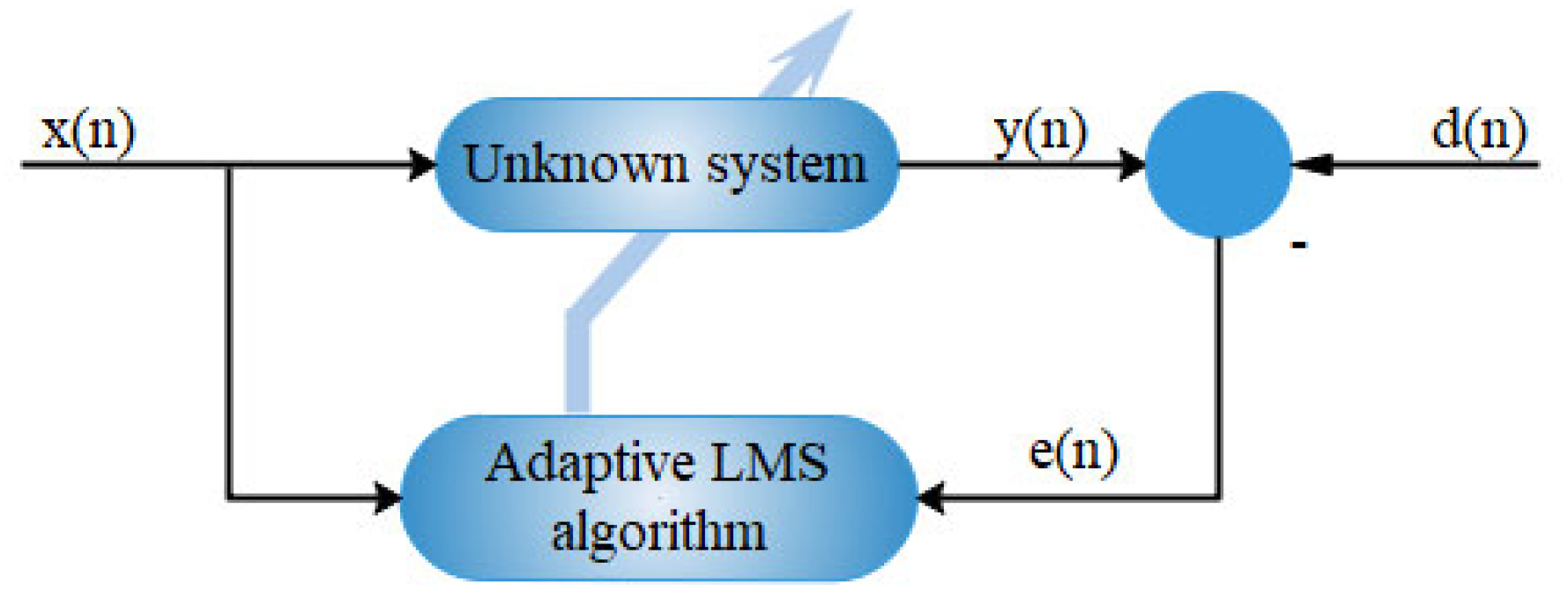
2.1. Principle of LMS Algorithm

The adaptive LMS algorithm is based on the Wiener filter and incorporates the gradient descent method. It minimizes the error between the filter output y(n) and the desired output d(n) by adjusting the weight vector. The cost function used is obtained as follows:

$$J(n)=\frac{1}{2}{e}^2(n)$$

(1)

By taking the gradient of $J(n)$ with respect to $w(n)$, the weight update formula for the standard LMS algorithm can be obtained as follows:

$$\begin{array}{cc}\hfill w(n+1)& =w(n)+\mu (-\nabla J(n))\hfill \\ & =w(n)+\mu e(n)X(n)\hfill \end{array}$$

(2)

The schematic diagram of system identification based on the LMS algorithm is shown in Figure 1.

The detailed model of the adaptive LMS algorithm is depicted in Figure 2.

In summary, the LMS algorithm consists of two main processes: filtering and adaptive adjustment. The specific steps are as follows:

(1)

Determine the parameters: the global step size parameter β and the number of taps in the filter.

(2)

Initialize the initial value of the filter.

(3)

Algorithm operation process:

• Filter output: $y(n)=w^T(n-1)X(N)$
• Error signal: $e(n)=d(n)-y(n)$
• Weight coefficient update: $w(n)=w(n-1)+\mu e(n)X(N)$

Here, $X(N)={\left[x(n),x(n-1)\cdots ,x(n-k+1)\right]}^T$ represents the input of each tap of the $k$-th order filter.

2.2. Principle of Variable-Step LMS Algorithm

By using the Lagrange multiplier method to find the extreme value under the constraint, the following equations are derived:

$$\Delta w(n+1)=w(n+1)-w(n)$$

(3)

$$d(n)=w^T(n+1)X(N)$$

(4)

where Equation (3) is the formula for the incremental weight, and Equation (4) is the expected value (the constraint). Therefore, the cost function obtained using the Lagrange multiplier algorithm is as follows:

$$J(n)={\Vert \Delta w(n+1)\Vert }^2+\lambda \left[d(n)-w{(n+1)}^{T}X(N)\right]$$

(5)

where $\lambda$ is the Lagrange multiplier coefficient. If we take the partial derivative of $J(n)$ about $w(n+1)$ and obtain 0, then we have the following:

$$\frac{\partial J(n)}{\partial w(n+1)}=2\left[w(n+1)-w(n)\right]-\lambda X(N)\stackrel{}{\to }=0$$

$$w(n+1)=w(n)+\frac{1}{2}\lambda X(N)$$

(6)

Based on the above formula, there is the following expression:

$$\begin{array}{cc}\hfill e(n)& =d(n)-y(n)=w^T(n+1)X(N)-w^T(n)X(N)\hfill \\ & =\frac{1}{2}\lambda {\Vert X(N)\Vert }^2\hfill \end{array}$$

(7)

The Lagrange coefficient $\lambda$ can be obtained as follows:

$$\lambda =\frac{2e(n)}{{\Vert X(N)\Vert }^2}$$

(8)

The new normalized weight update algorithm obtained from the above formula is as follows:

$$w(n+1)=w(n)+\frac{\mu }{\gamma +{\Vert X(N)\Vert }^2}e(n)X(N)$$

(9)

where $\mu$ is the iterative step size. To prevent the divergence of the algorithm when $x(n)$ is small, a parameter $\gamma$ (0 < $\gamma$ < 1) is introduced. It is evident that the iterative step size of the algorithm remains constant. The logistic function is a widely used nonlinear mapping S-shaped function in deep learning. Its general form is as follows:

$$f(x)=\frac{1}{1+e^x}$$

(10)

Therefore, the functional model with the step size varying with the error is as follows:

$$\mu (n)=\frac{1}{1+\exp (-\left|e(n)\right|)}-0.5$$

(11)

Considering Equations (9)–(11) comprehensively, the improved model of the step size varying with the error is obtained as follows:

$$\mu (n)1=\frac{\alpha \left[1-\exp (-\beta {\left|e(n)\right|}^2)\right]}{\gamma +{\Vert X(N)\Vert }^2}$$

(12)

2.3. Principle of Variable-Step LMS Algorithm Based on Incidental Momentum Term

The momentum “accumulates” historical gradients. Therefore, when the weight iteration algorithm includes a momentum term, the weight increment at previous moments will affect the weight change at the current moment. A larger forgetting factor indicates that the weight increment at previous moments has a greater impact on the weight change at the current moment. This discussion only focuses on the impact of the weight increment at the previous moment on the weight increment at the current moment. The new weight algorithm proposed is obtained as follows:

$$\left\{\hspace{1em}\begin{array}{cc}\hfill \Delta w(n{)}^{\prime }& =\Delta w(n)+\theta \Delta w(n-1)\hfill \\ & =\mu e(n)X(N)+\theta \Delta w(n-1)\hfill \\ \hfill w(n)& =w(n-1)+\Delta w(n{)}^{\prime }\hfill \end{array}\right.$$

(13)

where $\theta$ is the forgetting factor. Obviously, if the weight increment $\Delta w(n)$ at the current moment is in the same direction as the weight increment $\Delta w(n-1)$ at the previous moment, the magnitude of the weight increment will increase. If they are in the opposite direction, the magnitude of the weight increment will decline. Based on the above discussions, the process of the variable-step LMS algorithm with a momentum term can be obtained as follows:

(1)

Determine the parameter: the number of taps for the filter.

(2)

Initialize the initial value of the filter.

(3)

Algorithm operation process:

• Filter output: $y(n)=w^T(n-1)X(N)$
• Error signal: $e(n)=d(n)-y(n)$
• Step size adjustment: $\mu (n)1=\frac{\alpha \left[1-\exp (-\beta {\left|e(n)\right|}^2)\right]}{\gamma +{\Vert X(N)\Vert }^2}$
• Weight coefficient update: $\begin{array}{l}\Delta w(n)=\mu e(n)X(N)+\theta \Delta w(n-1)\\ w(n)=w(n-1)+\Delta w(n)\end{array}$

3. Numerical Simulation and Verification

3.1. Determine the Optimal Algorithm Parameters

The standard wideband signal $x(t)$ is obtained as follows:

$$x(t)=\exp (i\times 2\pi \times (f_{0}t+\frac{1}{2}k{t}^2))$$

(14)

where $f_0$ is the starting frequency and $k$ is the rate of frequency change over time. Setting $f_0$ to 10 Hz, $k$ to 500, and the sampling period to 0.001 s, the standard LMS algorithm and the variable-step normalization LMS (VSNLMS) algorithm are used to filter the noisy signal $\mathrm{s}(t)$. The filtered signals ${\mathrm{s}}^{\prime }(t)$ and $x(t)$ are compared for their errors. Figure 3a shows the time domain of the original signal $x(t)$ and the noisy signal $\mathrm{s}(t)$ with white noise, and Figure 3b shows the Hilbert time-frequency energy.

As shown in Figure 4, the output error diagram of a filter pair based on the LMS algorithm and VSNLMS algorithm is shown.

Obviously, the output error of the VSNLMS algorithm is significantly smaller than that of the LMS algorithm, indicating that the VSNLMS outperforms the LMS in filtering. The Pearson correlation coefficient R between ${\mathrm{s}}^{\prime }(t)$ and $x(t)$ is calculated to evaluate the filtering performance of different algorithms. Moreover, to quantify the impact of parameter changes on the filtering performance of the VSNLMS algorithm, the control variable method is used to obtain the R value between ${\mathrm{s}}^{\prime }(t)$ and $x(t)$ when the parameters α, β, and γ range from 0.1 to 0.9. Finally, the optimal filtering parameters for the VSNLMS algorithm are determined. The formula for calculating the Pearson correlation coefficient is obtained as follows:

$$R=\frac{{\displaystyle \sum _{i=1}^n(x_i-\overline{x})(y_i-\overline{y})}}{\sqrt{{\displaystyle \sum _{i=1}^n{(x_i-\overline{x})}^2}}\sqrt{{\displaystyle \sum _{i=1}^n{(y_i-\overline{y})}^2}}}$$

(15)

where $x_i$, $y_i$, $\overline{x}$, and $\overline{y}$ represent the sample points and the corresponding means for the two datasets.

Table 1. Changes in correlation coefficient R values of LMS and VSNLMS algorithms under different parameter conditions.

Based on LMS Algorithm
R1					0.8822
VSNLMS algorithm, β, γ take 0.5, α take 0.1~0.9
R2	0.9505	0.9656	0.9718	0.9752	0.9774	0.9789	0.9801	0.9810	0.9817
VSNLMS algorithm, α, γ take 0.5, β take 0.1~0.9
R3	0.9507	0.9655	0.9716	0.9750	0.9772	0.9787	0.9799	0.9808	0.9815
VSNLMS algorithm, α, β take 0.5, γ take 0.1~0.9
R4	0.9779	0.9778	0.9777	0.9776	0.9775	0.9774	0.9773	0.9772	0.9771

shows the R values obtained based on the LMS and VSNLMS algorithms.

According to the above quantitative analysis, the optimal parameters for the VSNLMS algorithm are as follows: $\alpha =0.9$, $\beta =0.9$, and $\gamma =0.1$. On this basis, the impact of θ on the M-VSNLMS algorithm is further analyzed.

Table 2. Changes in correlation coefficient R values of LMS and M-VSNLMS algorithms under different parameter conditions.

LMS Algorithm
R1					0.8822
M-VSNLMS algorithm, α, β take 0.9, γ take 0.1, θ take 0.1~0.9
R5	0.9778	0.9792	0.9796	0.9811	0.9821	0.9831	0.9835	NaN	NaN

reports the R values obtained by the LMS and M-VSNLMS algorithms. By adjusting the value of θ, the variation trend of R with θ is investigated based on the conclusions in Table 1.

It can be observed from Table 1 and Table 2 that as the parameters α, β, and θ increase, the correlation coefficient R between the filter output sequence and the original sequence also increases, and the algorithm diverges when θ is set to 0.8 or 0.9. Nevertheless, the correlation coefficient R declines as the parameter γ increases. Figure 5 shows the relationship between the Pearson correlation coefficient R and values of the parameters α, β, γ, and θ obtained via the control variable method.

From Figure 5, it can be observed that the correlation coefficient between the output sequence of the M-VSNLMS algorithm and the original signal is much higher than the result of the LMS algorithm. Additionally, parameters α and β have the most significant impact on the algorithm, and the momentum term coefficient θ further improves the prediction accuracy of the algorithm. Although the increase in γ results in a decrease in prediction accuracy, this impact is slight.

The above analysis shows that the optimal parameters for the M-VSNLMS algorithm are as follows: $\alpha =0.9$, $\beta =0.9$, $\gamma =0.1$, and $\theta =0.7$. On the basis of the above conclusions, the LMS and M-VSNLMS algorithms are used to filter the noisy signal $\mathrm{s}(t)$. Figure 6 illustrates the convergence process of the weight values for both algorithms. For the LMS algorithm, since its weight increment is fixed-step, the weight convergence curve is smooth, but the convergence rate is obviously slow. And at the sampling time of 15 s, the weights are still in a slow iteration process. For the M-VSNLMS algorithm, since its weight increment is variable-step, the weight convergence curve is erratic, but the convergence rate is fast. At t1 = 1.5 s, the weight of each tap quickly converges, and at t1 = 4 s, the weight of each tap roughly converges to a stable state. These demonstrate that the M-VSNLMS algorithm not only has significantly smaller convergence errors compared to those of the LMS algorithm but also has a distinct advantage in terms of the convergence rate.

Figure 7 presents the performance of the LMS, VSNLMS, and M-VSNLMS algorithms in filtering the signal $\mathrm{s}(t)$. The results demonstrate that the M-VSNLMS algorithm has the best performance on original signal reconstruction and noise removal in the time domain, frequency domain, and energy distribution. Figure 7 shows the Hilbert time-frequency of the $\mathrm{s}(t)$ filtering results using different algorithms.

3.2. Example Validation

To verify the convergence of the proposed algorithm and the optimization effect of the above conclusions on the algorithm’s learning capability, the M-VSNLMS algorithm with $\alpha =0.9$, $\beta =0.9$, $\gamma =0.1$, and $\theta =0.7$ is used to identify the parameters of a dynamic system model.

$$y(k)+a_{1}y(k-1)+a_{2}y(k-2)=b_{1}u(k-1)+b_{2}u(k-2)+v(k)+d_{1}v(k-1)$$

Among them, when the model parameters are $a_1=-0.5$, $a_2=-0.2$, $b_1=1.0$, $b_2=1.5$, $d_1=-0.8$, $v(k)$ is Gaussian white noise with a mean value of 0 and variance of 0.01. The input signal u(t) adopts the white noise sequence. In Figure 8, the predicted results of the model are shown.

As shown in

Table 3. Comparison between system identification results and true values.

Estimated Parameters	a1	a2	b2	b1	d1
True value	−0.5	−0.2	1.0	1.5	−0.8
Estimated value	−0.5158	−0.2059	0.9671	1.4673	0.0044
Estimation error	0.0158	0.0059	0.0329	0.0327	0.8044

, the true values of the estimated parameters are compared with the estimated values.

As shown in Table 3, the identification accuracy of system model parameters is above 97%, while the identification accuracy of noise is only 0.55%, indicating a good ability to suppress noise, demonstrating the excellent system identification performance of the M-VSNLMS algorithm. In addition, the algorithm has poor performance in terms of noise model identification, indicating its good noise suppression ability.

3.3. Experimental Steps and Results

In order to verify whether the proposed algorithm has good application effects in engineering, instruments and equipment were built in the aerodynamic elasticity laboratory of CARDC, as shown in Figure 9. By applying the driving voltage to the actuator, the aircraft model is vibrated, and the vibration signals are collected in real-time. In Figure 9a,b, the schematic diagram of the experimental device and the schematic diagram of the measurement and control system are shown respectively.

In

Table 4. Measurement and control instrument information.

Components	Brand	Function
Computer operating system	Windows 7	Program running environment
DC stabilized power supply	DP832A	Provide stable power supply for the balance
Balance	ADAM-3016	Measuring force and torque signals
Strain signal acquisition module	PXIe-4339	Signal amplification and filtering
Filter	PFI- 28618-M102	Low pass
Controller	dSPACE-Microlabox RTI1202	A/D conversion, calculation control signal, D/A conversion
Power amplifier	E-481K023	Amplify control signal

, information on the selected measurement and control instruments is shown. The signal processing module uses a series of products from National Instruments (NI) in the United States, the controller is a product from dSPACE in Germany, and the actuator uses piezoelectric stacking materials from Physical Instruments (PI) in Germany.

As shown in Figure 10, the real-time data fitting results based on the traditional ARMAX algorithm and N4SID algorithm are as follows:

As shown in Figure 11, the real-time data fitting results of the data-driven self-learning algorithms LMS and M-VSNLMS are as follows:

Calculate the correlation coefficient ${\delta }_{xy}$ and mean square error MSE between the output data of the above four algorithms and the expected data.

$${\delta }_{xy}=\frac{Cov(X,Y)}{D_x{D}_y}=\frac{1}{n}{\displaystyle \sum _{i=1}^n\frac{X_i-\overline{X}}{\sqrt{\frac{{\displaystyle \sum _{i=1}^n{\left(X_i-\overline{X}\right)}^2}}{n}}}}\frac{Y_i-\overline{Y}}{\sqrt{\frac{{\displaystyle \sum _{i=1}^n{\left(Y_i-\overline{Y}\right)}^2}}{n}}}$$

(16)

$$MSE=\frac{1}{n}{\displaystyle \sum _{i=1}^N{\left(X_i-Y_i\right)}^2}$$

(17)

Among them, the correlation coefficient ${\delta }_{xy}$ is the ratio of the covariance of the output data and the expected data to the product of the expected values of the two. $X_i$, $Y_i$, $\overline{X}$, and $\overline{Y}$ respectively represent the sampling and average values of the output data and the expected data, and $n$ represents the sample data capacity. In

Table 5. Error analysis between model output value and expected value.

Mathematical Model	${\mathit{\delta }}_{\mathit{x}\mathit{y}}$	$\mathit{M}\mathit{S}\mathit{E}$	Mathematical Model Order	Complexity of Mathematical Models
ARMAX	0.8787	0.0042	19	Complex
N4SID	0.8981	0.0021	11	Complex
LMS	0.9687	0.0011	-	Simple
M-VSNLMS	0.9898	0.00039	-	Simple

, the experimental results of the four algorithms are compared.

From Table 5, it can be seen that the data fitting effect of the data-driven self-learning algorithm is superior to that of traditional algorithms, and the data fitting accuracy of the M-VSNLMS algorithm is higher than that of the LMS algorithm. This is consistent with the simulation results and also indicates that the M-VSNLMS algorithm has a stronger real-time identification ability for physical systems than the LMS algorithm. The mathematical model of traditional algorithms has a higher order, which makes the mathematical model more complex, and the correlation between the algorithm output data and the expected data is less than 0.9. The correlation between the output data based on self-learning algorithms and the expected data is above 0.95. The algorithm output data are obtained through the linear convolution operation, and the mathematical model structure of the algorithm is simple. Through the above experiments, it is shown that the algorithm proposed in this article has value for engineering applications.

4. Conclusions

(1)

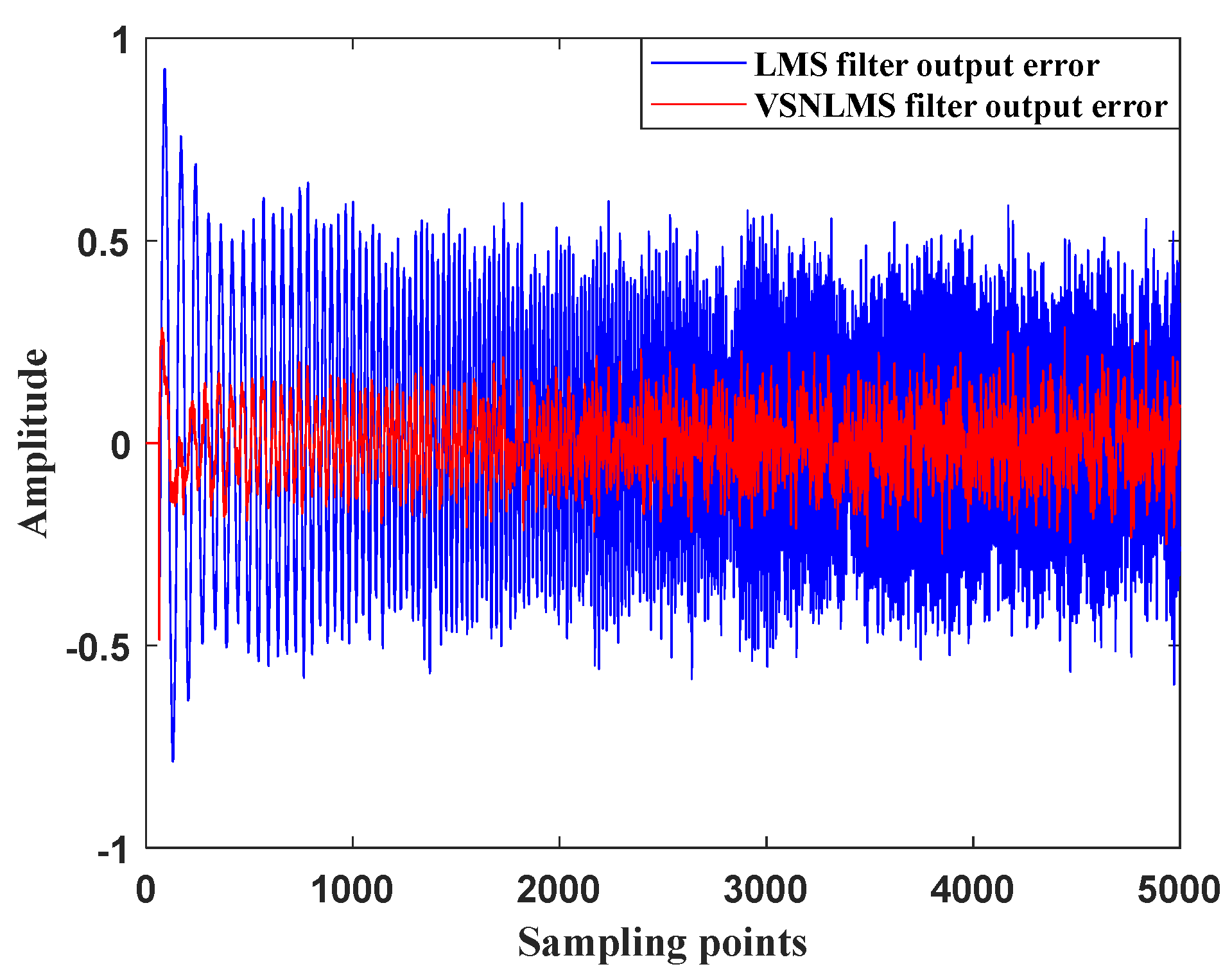
Based on the LMS algorithm, a variable-step-size normalization adaptive filter algorithm known as VSNLMS is developed to further minimize convergence errors in adaptive filtering. This algorithm utilizes the logistic function to establish a function model of step size varying with the error. The filtering results of the VSNLMS algorithm are compared to those of the LMS algorithm for wideband signals with noise. It is observed that the VSNLMS algorithm achieves significantly smaller convergence errors. The effects of the VSNLMS algorithm parameters (α, β, and γ) on the filtering results are investigated using the control variable method. On this basis, the optimal parameter values are determined.

(2)

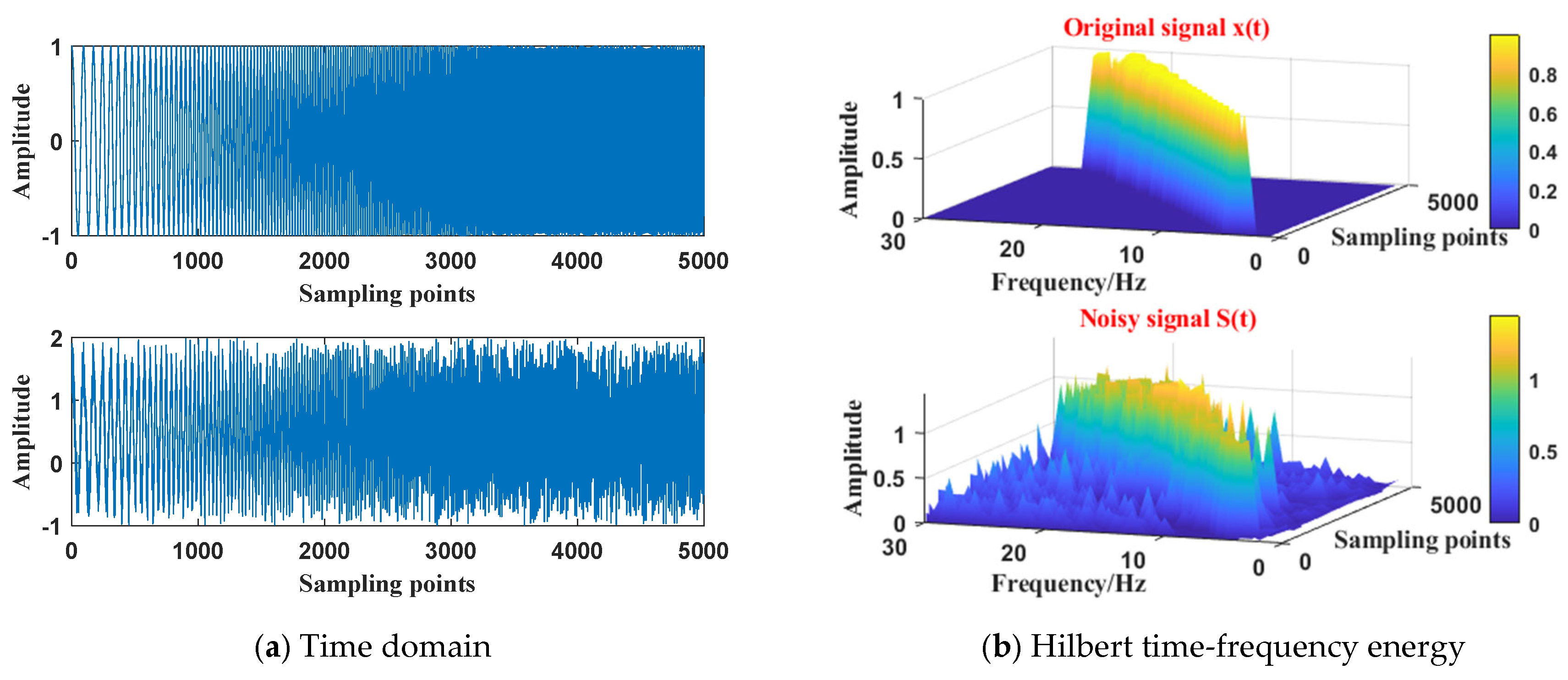
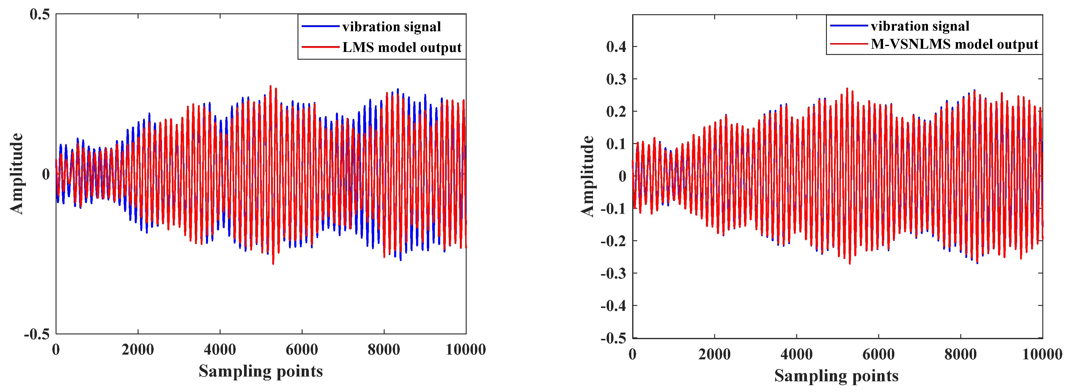
To accelerate the convergence of the algorithm, a momentum term θ is introduced into the VSNLMS algorithm, resulting in the modified VSNLMS (M-VSNLMS) algorithm. This term consists of a forgetting factor and a momentum term of weight increment from the previous moment. This modification enables the algorithm to anticipate changes in the error trend, leading to faster convergence. The effects of the M-VSNLMS algorithm parameter θ on the filtering results are investigated based on the above conclusion, and the optimal parameter values are determined. Moreover, the filtering results of the M-VSNLMS algorithm are compared to those of the LMS algorithm for wideband signals containing noise. The results demonstrate that the M-VSNLMS algorithm achieves signal reconstruction and effective noise suppression in the time domain, frequency domain, and energy distribution. Furthermore, it exhibits a significantly faster convergence rate compared to that of the LMS algorithm.

(3)

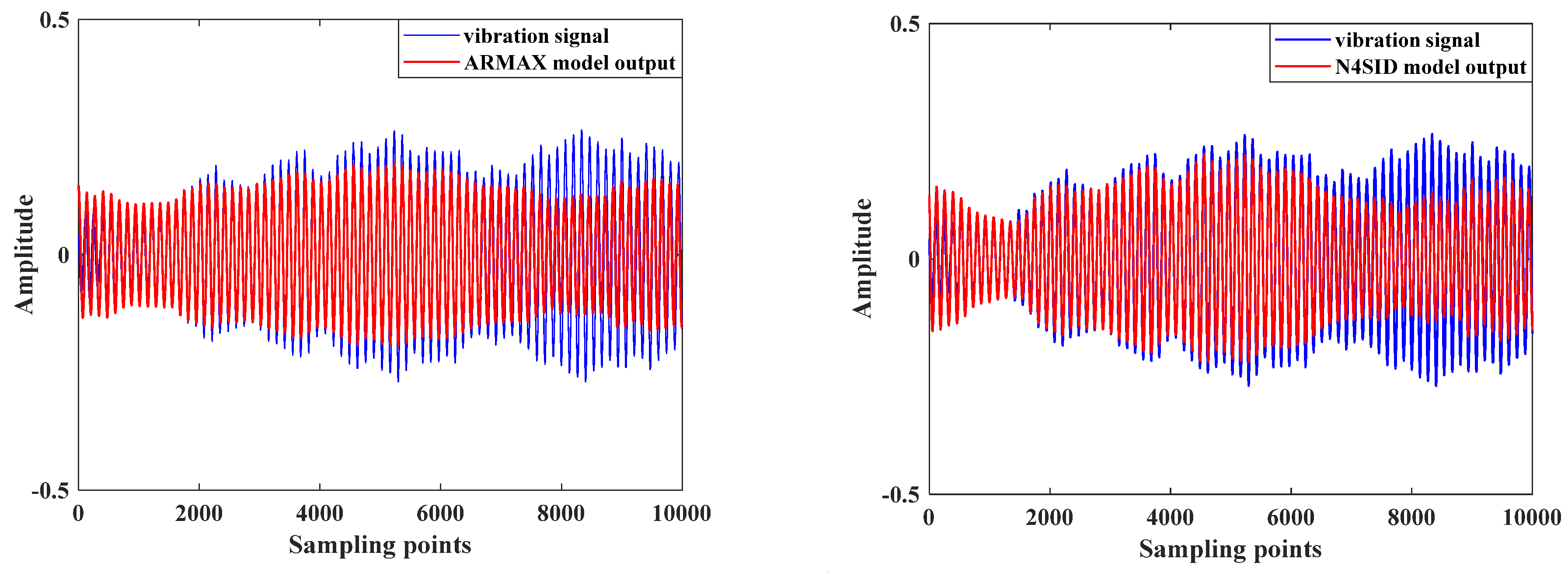
The M-VSNLMS algorithm is utilized to perform system identification on a noisy dynamic system mathematical model. The results show that the proposed algorithm can accurately identify the mathematical model with an accuracy of over 97%, while also suppressing the noise components in the logarithmic model by over 99%. Real-time vibration data fitting experiments were conducted in the aeroelastic laboratory of CARDC. The data fitting capabilities and mathematical model complexity of four algorithms, ARMAX, N4SID, LMS, and M-VSNLMS, were compared, indicating that M-VSNLMS has a higher real-time data fitting accuracy and lower-complexity mathematical models.

The weight update of the algorithm relies on the error gradient and the magnitude of the step size. However, for strongly nonlinear and intermittently active systems, the algorithm may encounter the local optimum of the error gradient or large fluctuations in the step size, leading to prolonged convergence or even divergence. To address this issue, further analyses are necessary regarding the computation and processing of the system input data in higher-dimensional spaces, so as to enable the identification and noise reduction of more complex systems. Notably, recent research has proposed algorithms such as Kernel Adaptive Filtering (KAF) and Convolutional Neural Network (CNN), which offer valuable insights in this domain.

References

1. Shen, F. Adaptive Signal Processing; Xi’an University of Electronic Science and Technology Press: Xi’an, China, 2001. [Google Scholar]
2. Wang, B.; Li, H.; Gao, S.; Zhang, M.; Xu, C. A variable step size minimum average p-norm adaptive filtering algorithm. J. Electron. Inf. Technol. 2022, 44, 661–667. [Google Scholar]
3. Widrow, B.; Hoff, M.E. Adaptive switching circuits. In Neurocomputing: Foundations of Research; MIT Press: Cambridge, MA, USA, 1988. [Google Scholar]
4. Xie, B.; Wang, N. Simulation research based on improved BP LMS adaptive filter algorithm. Comput. Digit. Eng. 2022, 50, 6. [Google Scholar]
5. Yasukawa, H.; Shimada, S.; Furukawa, I. Acoustic echo canceller with high speech quality. In Proceedings of the IEEE International Conference on Acoustics, Speech and Signal Processing, Dallas, TX, USA, 6–9 April 1987; pp. 2125–2128. [Google Scholar]
6. Widrow, B.; Mccool, J.; Ball, M. The complex LMS algorithm. Proc. IEEE 2005, 63, 719–720. [Google Scholar] [CrossRef]
7. Wang, B.; Chao, P.; Zhang, W.; Wang, J.; Jin, P.; Xie, F. Variable Step Size LMP Adaptive Filtering Algorithm Based on Improved Tanh Function. CN202111415232. X 25 February 2022. [Google Scholar]
8. Bouboulis, P.; Theodoridis, S.; Mavroforakis, M. The augmented complex kernel LMS. IEEE Trans. Signal Process. 2012, 60, 4962–4967. [Google Scholar] [CrossRef]
9. Zhang, S.; Sun, L.; Wang, X. The Application of a New Variable Step Size ELMS Algorithm in Noise Cancellation. J. Terahertz Sci. Electron. Inf. Technol. 2022. [Google Scholar]
10. Dai, C.; Fang, M. Vehicle mounted ANC simulation based on adaptive filtering algorithm. Model. Simul. 2023, 12, 366–379. [Google Scholar] [CrossRef]
11. Wu, L.; Nie, Y.; Zhang, Y.; He, S.; Zhao, Y. Adaptive filtering denoising method based on variational mode decomposition. J. Electron. Sci. 2021, 49, 1457–1465. [Google Scholar]
12. Tobar, F.A.; Kuh, A.; Mandic, D.P. A Novel augmented complex valued kernel LMS. In Proceedings of the 2012 IEEE 7th Sensor Array and Multichannel Signal Processing Workshop (SAM), Hoboken, NJ, USA, 17–20 June 2012; IEEE: Piscataway, NJ, USA, 2012; pp. 473–476. [Google Scholar]
13. Dai, Y.; Zhang, L.; Zhao, Z.; Shen, X. Wind-Tunnel Evaluation for an Active Sting Damper Using Multi-modal Neural Networks. AIAA J. 2020, 58, 1939–1948. [Google Scholar] [CrossRef]
14. Zhang, L.; Dai, Y.; Kou, X.; Yu, L.; Lu, B.; Shen, X. Research on an Active Pitching Damper for Transonic Wind Tunnel Tests. Aerosp. Sci. Technol. 2019, 94, 105364. [Google Scholar] [CrossRef]
15. Zhan, G.; Wu, Z. A New Variable Step LMS Adaptive Filtering Algorithm. J. Nav. Eng. Univ. 2006, 36, 109–112. [Google Scholar]
16. Lin, J.; Zheng, Y.B. Vibration suppression control of smart piezoelectric rotating truss structure by parallel neuro-fuzzy control with genetic algorithm tuning. J. Sound Vib. 2012, 331, 3677–3694. [Google Scholar] [CrossRef]
17. Zhang, X. Kernel Adaptive Filtering Algorithm and Its Application in Noise Cancellation and Channel Equalization. Xihua University: Chengdu, China, 2017. [Google Scholar]
18. Qian, F.; Huang, J.; Qin, X. Research on system identification algorithm based on robust optimization. Acta Autom. Sin. 2014, 40, 988–993. [Google Scholar]
19. Feng, D. Research on complexity, convergence and computational efficiency of system identification algorithm is published first. Control. Decis. Mak. 2016, 31, 1729–1741. [Google Scholar]
20. Ji, Z. Comparison and simulation of system identification algorithms based on correlation analysis. Comput. Knowl. Technol. Acad. Exch. 2016, 12, 253–254. [Google Scholar]
21. Liu, W.; Zhou, M.D.; Wen, Z.Q.; Yao, Z.; Liu, Y.; Wang, S.H.; Cui, X.C.; Li, X.; Liang, B.; Jia, Z.Y. An Active Damping Vibration Control System for Wind Tunnel Models. Chin. J. Aeronaut. 2019, 32, 2109–2120. [Google Scholar] [CrossRef]
22. Dai, Y.K.; Shen, X.; Zhang, L.; Yu, Y.; Kou, X.P.; Yu, L. System Identification and Experiment Evaluation of a Piezoelectric-Based Sting Damper in a Transonic Wind Tunnel. Rev. Sci. Instrum. 2019, 90, 075102. [Google Scholar] [CrossRef] [PubMed]
Figure 1. Schematic diagram of system identification based on LMS algorithm.
Applsci 13 12077 g001
Figure 2. Schematic diagram of LMS algorithm model.
Applsci 13 12077 g002
Figure 3. Time domain and Hilbert time-frequency energy of original signal and noisy signal.
Applsci 13 12077 g003
Figure 4. Schematic diagram of filtering error based on LMS and VSNLMS algorithms.
Applsci 13 12077 g004
Figure 5. The correlation between R and parameters α, β, γ, and θ.
Applsci 13 12077 g005
Figure 6. Weight convergence process of LMS and M-VSNLMS algorithms.
Applsci 13 12077 g006
Figure 7. Hilbert time-frequency plots of S(t) filtering results using different algorithms.
Applsci 13 12077 g007
Figure 8. s ( t ) and e ( t ) time domain and convergence of various parameters.
Applsci 13 12077 g008
Figure 9. Schematic diagram of testing instruments.
Applsci 13 12077 g009
Figure 10. Real-time data fitting results of ARMAX and N4SID algorithms.
Applsci 13 12077 g010
Figure 11. Real-time data fitting results of LMS and M-VSNLMS algorithms.
Applsci 13 12077 g011