Abstract
The study of airspace sector demarcation can help controllers to deal with complex air situations, provide reference for air traffic control services, reduce the workload of controllers, and ensure safe and efficient airspace operation. Based on complex network theory, this paper proposes a sector division method based on a mean shift clustering algorithm and a Voronoi diagram. Firstly, a flight conflict network is constructed based on the structural characteristics of the airborne flight situation, combined with the three-dimensional velocity barrier method and the aircraft protected area model. Secondly, six network topology indexes, such as the total node degree, average point strength and network density, are selected to construct the flight-situation-assessment index system, and the busy and idle time segments of the airspace are divided according to the comprehensive network indexes; finally, based on the historical flight data, the airborne aircraft in the busy and idle time segments are clustered using the mean shift clustering algorithm and the Voronoi diagram method, respectively, so as to obtain a sector division scheme. The simulation results show that this method can equalize the network topology indexes and provide a reference for the scientific allocation of controllers’ energy.
1. Introduction
After the COVID-19 epidemic, the civil aviation transportation industry has rapidly recovered and entered a new strong development phase; the airspace operation environment is becoming more and more complex, the air traffic flow continues to increase, and the problems arising from various aspects, such as air transportation efficiency and flight safety, are becoming more and more serious. In order to sort out the air traffic, we usually divide the airport area into multiple sectors, which are commanded and deployed by multiple controllers. However, the number of aircraft in different sectors may vary greatly at the same time, which leads to a very heavy load on the busy controllers in some sectors and poses safety risks. The scientific and reasonable division of airport sectors can effectively solve this problem and ensure flight safety, which makes sector optimization a hot research topic in the industry [1].
At present, the research on airspace sector-delineation technology at home and abroad mainly adopts mathematical modeling methods, such as graph theory and clustering and intelligent optimization algorithms. Delahaye et al. establish Voronoi polygons by taking randomly generated points in the two-dimensional airspace as the clustering centers or nodes, and determine the sector-delineation scheme by adopting genetic algorithms with the goal of balancing the control loads in each polygon [2]. On the basis of this, Yousefi proposed a sector-delineation method based on controller workload by dividing the airspace into grids according to flight safety intervals and flight route requirements [3]. Brinton proposed and analyzed an algorithm for the optimal sector delineation of airspace with the goal of balancing dynamic density, and clustered the spatial positions of the recorded aircraft based on the nature of the metrics and the location of the airspace boundaries [4]. Gianazza combined the tree search algorithm with neural network to explore the division method of airspace block combination on the basis of airspace segmentation [5]. Han Songchen applied the theory of the variable precision rough set to derive the optimal number of sectors in various cases, and then derived the final optimal combination of sectors, which proved the practicability of this method [6]. Luo Jun et al. use Voronoi diagram and a particle-swarm optimization algorithm to balance the workload of each waypoint, and establish a sector-combination optimization model [7]. Flener et al. propose a sector-delineation method based on the workload of control [8]. Sergeeva et al. design a sector-delineation and optimization algorithm based on the genetic algorithm for 3D airspace [9]. Kang Jifang analyzes the complexity factors of the airspace using principal component analysis, and selects a sector-delineation algorithm suitable for the structural characteristics of the airspace through a comprehensive description and comparison of different intelligent algorithms to select sector-delineation algorithms suitable for the structural characteristics of the airspace for different airspaces [10]. Yan Xinmiao proposes a method based on historical trajectory radar data, extracting navigational information, and realizing the sector delineation of terminal airspace through data mining [11]. Most current sector delineation mainly focuses on the three aspects of reducing air traffic complexity, equalizing controller load, and improving airspace capacity.
The current airspace sector-delineation research mainly focuses on modeling the target airspace based on known airspace information in order to achieve the balance of sector control load and air traffic safety. When considering the sector-delineation method, it is proposed to introduce the Voronoi diagram for sector delineation, which is a widely used spatial topology, firstly proposed by the Dutch meteorologist A.H. Thiessen, and a spatial partitioning technique that regularly divides the plane [12,13]. Voronoi diagrams in the spatial sectioning equipartition well match the demand of airport area for sector division; the core problem of using this method for airspace sector division is to select a suitable method to obtain the Voronoi-diagram-generating elements so as to obtain the airspace sector scheme. Based on this, Trandac used airports, waypoints, and intersections as the center points to generate Voronoi diagrams in the controlled airspace [14]. Li used the spectral clustering method to based on the static structure of the airspace to build a weighted graph model, which is divided into convex polygons with the same control loads to generate a defined sector-division scheme [15]. Soh used a spectral clustering algorithm to bisect the airspace, followed by a weight-balancing algorithm to balance the weights of the obtained subgraphs [16]. Lin Fugen et al. improved the K-means algorithm by introducing weighting factors and capacity margins to determine reasonable cluster centers, and used the Voronoi diagram partitioning idea to achieve sector division [17].
The above methods are based on the fixed static route structure, and the clustering algorithm is selected or the generating elements are obtained directly according to the fixed position, and the control sector-delineation scheme is obtained with the goal of balancing the controller load. In order to better fit the actual airspace structure, this paper considers obtaining the historical air-traffic condition data of military airspace, quantifying the comprehensive index of the flight conflict network, clustering the air situation to obtain the Voronoi diagram generator, and then realizing the goal of balancing the control load.
In view of the above problems, this paper proposes a control-sector planning method based on a mean shift clustering algorithm. Firstly, based on the flight-conflict network, six network topology indicators are comprehensively considered to distinguish the sector idle time segment and busy time segment. Secondly, EM clustering is used to obtain the distribution of aircraft node-area centers, and the clustering method of the mean shift algorithm is used to obtain the node-area centers for the clustering center. Finally, the clustering center is used as a generating element using the Voronoi diagram method to obtain the new sector planning scheme.
2. Flight Conflict Network
In order to analyze the complexity of the air traffic situation and reasonably divide the sectors between idle and busy time, the flight conflict network is constructed using the complex network theory. The flight conflict network is a complex network that takes the conflict relationship between aircraft in the airspace as the research object, where denotes the set of nodes composed of aircraft in the network; is the set of connecting edges reflecting the conflict relationship between aircraft; and is the set of connecting edge weights reflecting the urgency of potential conflicts.
2.1. Determine Network Edges
In the flight conflict network, the connecting edges between nodes represent potential conflicts. Therefore, two conditions need to be satisfied for nodes in a flight conflict network to constitute edges: firstly, the corresponding aircraft of the nodes are relatively close to each other in terms of their positions; secondly, the speed barrier relationship is satisfied by the determination of the speed barrier model.
Aircraft are required to maintain a certain vertical or horizontal separation from each other during operation, and an ellipsoidal flight protection zone is established for airborne targets, as shown in Figure 1, with the equatorial radius of the zone a = b = , and the polar radius c = .
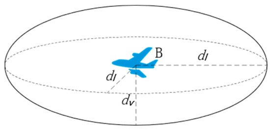
Figure 1.
Ellipsoidal flight protection zone.
Let the coordinates of aircraft B be a. The expression for the ellipsoid surface of the protected area is:
No conflict exists when the vertical separation between aircraft is greater than 300 m, so = 10 km, = 300 m is taken.
The velocity barrier method limits the relative velocity range of potential conflict of the target in the two-dimensional plane according to the geometric rules, and judges that it will be in conflict when its velocity relative to the obstacle is in the range. Since the airspace in which the aircraft operates is a three-dimensional space, the velocity barrier method is extended to three dimensions and the protected area is ellipsoidal in general. As shown in Figure 2, the relative velocity can be regarded as the velocity of aircraft A relative to B when aircraft B is at rest. When the direction is within the angle range of the three-dimensional velocity barrier cone, it means that if the current state of motion is not deployed, aircraft A will enter the flight protection zone of B and a flight conflict will occur.
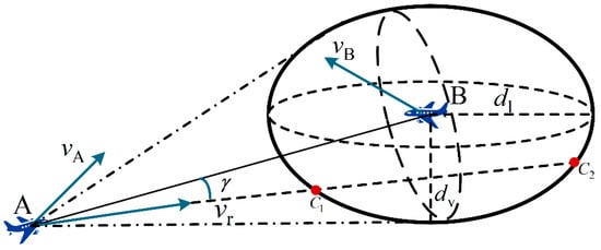
Figure 2.
Three-dimensional speed barrier conflict-detection model.
Let the three-dimensional coordinates of aircraft A be , and the direction vector of be . Then, according to the pointwise equation of the three-dimensional straight line, we have:
where denotes the coordinates of aircraft A; is the direction vector of . To associate the surface aspect (1) with the linear Equation (2), if there are two solutions, it means that there are two intersections, C1 and C2, between the flight protection zone of aircraft B and the line where is located; at the same time, if there is that holds, i.e., , then the direction of is inside the cone of the velocity barrier, and the nodes of the aircraft, A and B, form a connecting edge between each other.
is the angle between the relative velocity and the position vectors AB of aircraft A and B; |AB| denotes the distance between A and B.
2.2. Determine the Edge Weight
The contiguous edges of the flight-conflict network represent potential flight conflicts between aircraft in the airspace, and the edge weights should reflect the urgency of the conflict. Definition is the time when an aircraft maintains its current flight status and a conflict is expected to occur. When designing the weights of the edges, it is necessary to satisfy: (1) the smaller the distance between aircraft, the larger the relative speed, the more urgent the conflict, the larger the weights of the edges, i.e., the edge weights increase with the decrease in ; (2) as decreases, the urgency of the flight conflict is changing more and more drastically, and the weights are increasing more and more; (3) considering the principle of the speed obstacle law and the practical significance of the flight conflict, the weights of the edges should be positive value.
In summary, define the network edge rights:
Selecting the negative exponential function of the predicted conflict time as the weight has the following advantages: (1) The negative exponential function is a decreasing function on its domain. The longer the is, the smaller the weight is, and the weaker the conflict intensity is. (2) When forming the edge, the value of is greater than 0, so the value range of the negative exponential function is [0,1], which can play a role in uniting the weights. (3) The absolute value of the slope of the negative exponential function increases gradually with the decrease in the independent variable, which can reflect that the urgency of the potential flight conflict changes fiercely in the process of decreasing, which is consistent with the actual conflict situation.
3. Idle/Busy Time Segmentation
Airspace sectors in idle or busy time segments change air posture as the number, speed and heading of aircraft change. In order to accurately assess the airspace traffic and conflict situation, and to divide the sector to meet the requirements of busy/idle time operation, six topological indicators reflecting the local and global information of the airspace: total node degree, average node degree, average point strength, average weighted aggregation coefficient, network density, and network efficiency are selected as the influencing factors to divide the idle/busy time period.
3.1. Selection of Assessment Indicators
In order to comprehensively assess and classify the air traffic operation posture, six complex network characteristic indicators that can reflect the characteristics of the airspace conflict network from multiple perspectives are selected to describe the flight posture.
- 1.
- Total Node Degree
Degree is a key attribute of a node that indicates the number of links between that node and other nodes. In a conflict network, the degree value reflects the number of conflicts between one aircraft and other aircraft, and most intuitively reflects the local conflict situation, denoted by :
is the degree value of node i, N is the total number of nodes in the network, denotes the connectivity of two nodes, if connected and otherwise.
The total node degree reflects the total number of conflicts in the network; is denoted by:
- 2.
- Average Node Degree
On the basis of the degree value, for networks, the average degree is an important attribute of the network, indicating the average number of links between each node and other nodes throughout the network. In a conflict network, the average degree value can reflect the average number of conflicts each aircraft forms with its surrounding aircraft, denoted by :
- 3.
- Average Point Intensity
Point strength is the expression of the degree value after weighting; the index can not only reflect the number of neighboring nodes, but also reflect the degree of influence on the node around the node. In the conflict network, the average point strength can reflect the urgency of the conflict, and indirectly represents the average pressure of control deployment, which is denoted by :
is the connection relationship between two nodes, if connected, otherwise; is the edge right between nodes , .
- 4.
- Average Weighted Aggregation Factor
The weighted aggregation coefficient is a weighted expression of the ordinary aggregation coefficient, and a single value indicates the degree of aggregation at the location of a node and the degree of proximity between nodes, while the average weighted aggregation coefficient can reflect the degree of aggregation of the whole network. In a conflict network, this value can describe the degree of conflict aggregation of the network as a whole, which is denoted by :
is the weighted aggregation factor, calculated as follows:
is the degree of node ; is the point strength of node ; is the number of connected triples; , are the neighbor nodes of node .
- 5.
- Network Density
In the flight conflict network, the network density can be used to describe the denseness of the interconnecting edges between the nodes in the network, and the value can reflect the degree of saturation to the flight posture, denoted by :
L is the actual number of connected edges in the network.
- 6.
- Network Efficiency
The network efficiency visualizes the connectivity of the entire network; the efficiency between two nodes is expressed as the reciprocal of the distance to each other, while the efficiency of the entire network is the average of the efficiencies between every two pairs of nodes. In the conflict network, this value can easily represent the spreading breadth of the aircraft conflict, defined as:
is the shortest path between two nodes , . The higher the network efficiency NE, the closer the connection between the nodes, and the network is relatively more complex.
3.2. Integrated Network Indicator Classification
The six assessment indicators do not affect the flight attitude independently, but interact with each other and jointly affect the good or bad flight attitude at different times. The multi-factor interaction matrix (MFIM) was first applied to geological system engineering [18]. It not only considers the influence of each parameter on the system, but also reflects the influence and interaction between multiple factors. It is an effective method for the analysis of complex system problems.
The MFIM method mainly includes three processes: (1) encoding the multi-factor interaction matrix; (2) Calculate the subjective and objective influence degree of each index; (3) Allocate the weight of each index. This method can fully explore the relationship between indicators and analyze the internal factors of complex systems. However, the expert scoring method is usually used in matrix coding. This method is too subjective and lacks scientificity to some extent. Therefore, we wish to improve the coding method. The first step is to place the influencing factors on the main diagonal of the matrix (the order can be interchanged).
The maximal information coefficient is an effective method for determining the correlation between two variables [19]. Most correlation analysis finds it difficult to explore the nonlinear relationship between variables [20]. However, MIC can not only find linear and nonlinear correlations in the data, but also explore the potential non-functional correlations between them. If there is a connection between the two variables, the network partition of the scatter diagram composed of the two points can always have a suitable division method to reflect its relevance. The specific description is as follows:
Suppose that there exists a data set D, which contains two two-dimensional data variables x and y; then, the mutual information of x and y can be expressed as:
In the formula, is the joint probability distribution of x and y; increases with the increase in the correlation between x and y.
Since the calculation of the joint probability distribution is difficult, the scatter plot of the x-y data is meshed, and each continuous x (or y) is divided into the corresponding column x group (or row y group), thereby obtaining a new X, Y grouping. The mutual information calculation based on this is as follows:
Further, the correlation between the two variables MIC is defined as:
In the formula, the value of B is the 0.6 power of the sample size N, and the value of MIC is in the range of [0,1]. A higher MIC value indicates that the correlation between variables is stronger.
In addition, the position of the triangle on the main diagonal of the matrix (the blue part of the graph) is filled with the evaluation value A, and the Delphi 0–1 scoring method [21] is used to invite multiple experts to conduct independent scoring and evaluation. Describe the strength relationship between the indicators; the closer the value is to 1, the more important it is, and the less important it is.
The evaluation value on the non-main diagonal line of each row indicates the influence of the main diagonal factor on other factors, that is, the subjective effect. The code on each column of non-main diagonal indicates that the main diagonal is affected by other factors, that is, the objective effect. For example, represents not only the subjective influence of factor on factor in the horizontal direction, but also the objective influence of factor on factor in the vertical direction. Therefore, the multi-factor interaction matrix is asymmetric.
According to the construction principle of interaction matrix, the degree of subjective and objective effects of influencing factor i can be calculated according to the following formula:
In the formula, n is the number of influencing factors; and are the degree of subjective effect and objective effect of factor i in MFIM, respectively. and are the sum of the subjective and objective effect weights of all influencing factors; is the weight value of each index combined with subjective and objective influence.
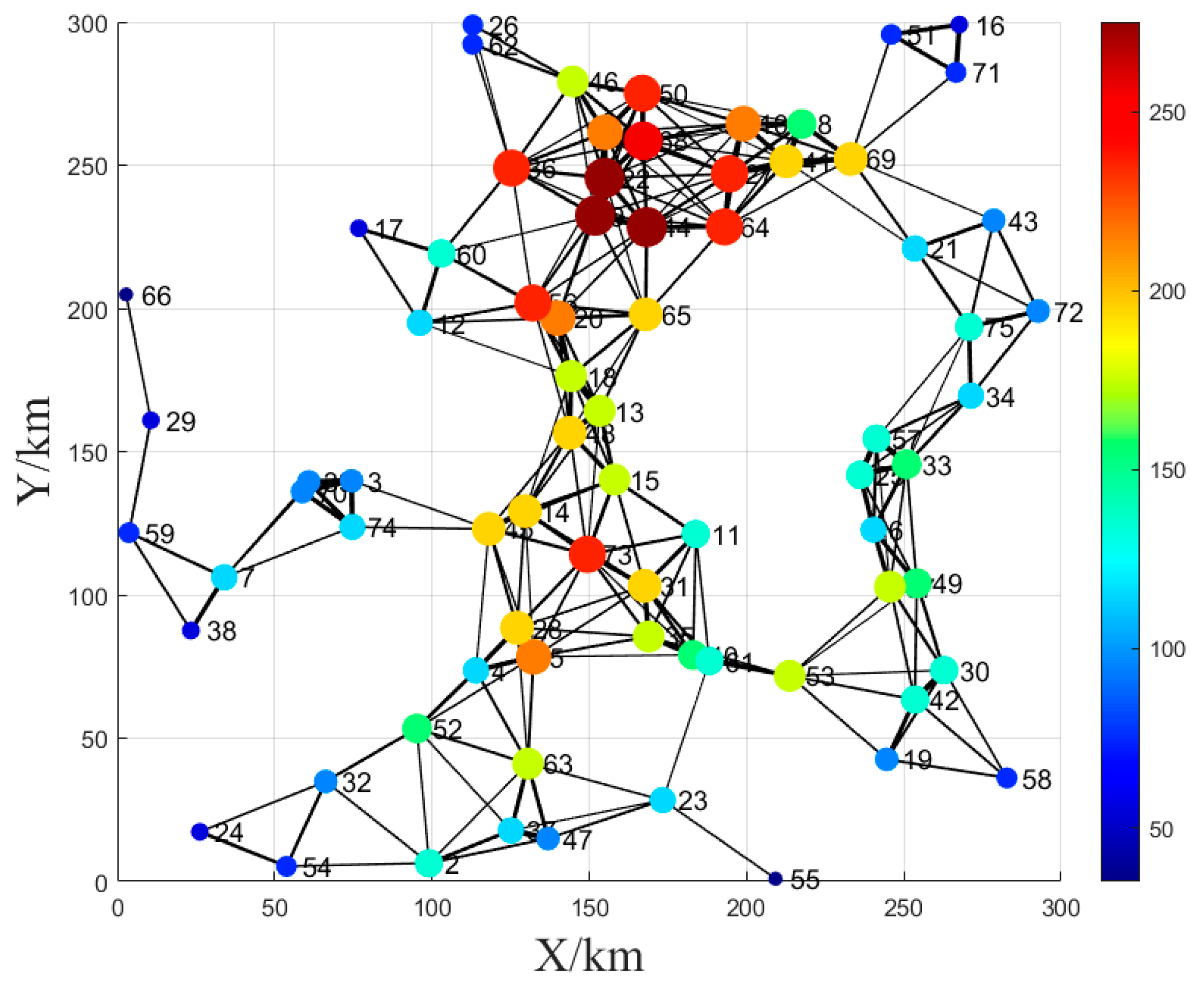
The MATLAB R2020b software is used to simulate the conflict network generated by the airspace in Figure 3, which contains 75 nodes. After visualization, the depth of the node color is set according to the degree value. The larger the degree value is, the deeper the color is, indicating that the conflict is more serious. The thickness of the edge represents the urgency of the conflict. The thicker the edge is, the more urgent the conflict is. The computational complexity metrics are shown in Table 1.

Figure 3.
Conflict network diagram.

Table 1.
Network complexity index.
The multi-factor mutual matrix of the six indicators calculated by this method is shown in Figure 4. The blue part is the expert scoring weight, and the green part is the maximum information coefficient weight.
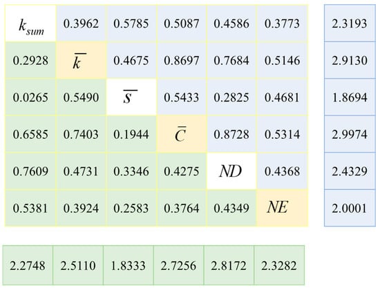
Figure 4.
Multi-factor interaction matrix for evaluation indicators.
According to the MFIM method, the final weights and the order of importance of the six indicators were (2.86) > (2.71) > (2.63) > (2.30) > (2.16) > (1.85). Each evaluation indicator was normalized to obtain a constant number of weights. The weighting of the combined six indicators constitutes the comprehensive network metrics (CNM) for evaluating the flight posture, and the CNM can be expressed as:
This index can comprehensively describe the flight conflict situation and flight posture in the airspace, using MATLAB software to simulate the airspace to generate 100 conflict networks that reflect the air operation situation. The conflict network setting rules are as follows: randomly generate 10–100 aircraft nodes, use the above aircraft protection area model and three-dimensional velocity obstacle method to judge the conflict relationship between aircraft, calculate the indicators in different conflict networks as sample sets, and calculate the comprehensive network indicator values of each conflict network. At the same time, three experts in related fields are invited to evaluate the flight situation and divide it into two different periods: busy/idle. The indicators and expert scoring are shown in Table 2.
Table 2.
Sample set.
The comprehensive network index is corresponding to the time-period division. The specific numerical division of the evaluation index is bounded by the value of 4. The comprehensive network index is greater than 4 and is defined as the busy period, and less than 4 is defined as the idle period.
4. Sector-Delineation Method Based on Mean Shift Clustering Algorithm
Obtain the flight radar data of the control area, record the radar data once in 10 min intervals in the busy and idle time segments according to the comprehensive network index, and collect the position information of all the aircraft in each radar data, with denoting the aircraft in the control area in the th moment of the record, and and denoting the nodes of the aircraft.
4.1. Integrated Network Indicator Classification
Firstly cluster analysis of aircraft nodes is carried out and the distribution of regional centers of aircraft nodes is obtained by clustering with an EM algorithm. The EM algorithm [22] is an iterative algorithm for the maximum likelihood estimation of the probability model parameters with hidden variables. It is a kind of algorithm in unsupervised learning. It has the advantages of stable and accurate calculation results and self-convergence.
The first step of the EM algorithm is to compute the expectation (E) and then maximize (M) the parameter found at step E. The parameter estimates found on step M are used in the next step of computation at step E. The process keeps on alternating until it converges
Step E: In spatial partitioning, EM searches for node clusters, by determining the parameters of the probability density function suitable for a given node set, and assigns nodes to different clusters; each cluster is modeled by a probability distribution. Each node approximately obeys the normal distribution. Therefore, assume that the joint distribution of latent variables and special variables . Calculate the sample weights of the kth (k is the number of clusters) normal distribution of the aircraft node sample :
Step M: Update clustering parameters:
, . Equations (25) and (26) are repeated until the difference of K sample weights is less than the given threshold, and the final estimate is obtained. The EM algorithm can be implemented by the normal distribution model to obtain the probability that each node belongs to each cluster, continuously update the estimated parameters, and then gradually modify the center value of each cluster. Finally, the classical maximum likelihood algorithm is used to obtain the regional node center.
4.2. Clustering Method Based on Mean Shift Algorithm
The mean shift algorithm [23] is the application of kernel density estimation in the feature space of the climbing algorithm. Its algorithmic idea is to assume different clusters of datasets in line with different probability density distributions (to find the fastest direction of any sample point density increase); the sample density of the region corresponds to the center of the cluster class, so that the sample point will ultimately converge in the local density of the largest place, and the convergence of the same local maximum value of the sample point is considered to be a member of the same cluster, based on this principle. The mean shift algorithm can be used for clustering, image segmentation, tracking, and so on.
When the mean shift algorithm is applied to the sector division, the center of the regional node obtained in the previous section is x, and the kernel function is . The basic mean shift vector is of the form:
Adding kernel functions and sample weights to the basic mean shift vector form yields the following improved mean shift vector form:
is the weight of each regional center, and for any regional center in the graph, its weight value is defined as the sum of the point strengths of the aerial vehicle nodes contained in that regional center:
The center of the region is selected as the seed point, is the tolerance error, and the mean shift algorithm implements the clustering of the center of the region according to the following steps:
Step 1: Calculate from the initial region center and assign to .
Step 2: Determine the move step and compute for the next region center.
Step 3: If , mark the center of the region and end the loop by assigning all the passed region centers from the start point with the same marking of the marked region center; otherwise, continue with steps 1 and 2 until all the nodes have been marked.
Step 4: Merge the homogeneous regions to obtain the clustering center.
4.3. Sector-Delineation Method Based on Voronoi Diagrams
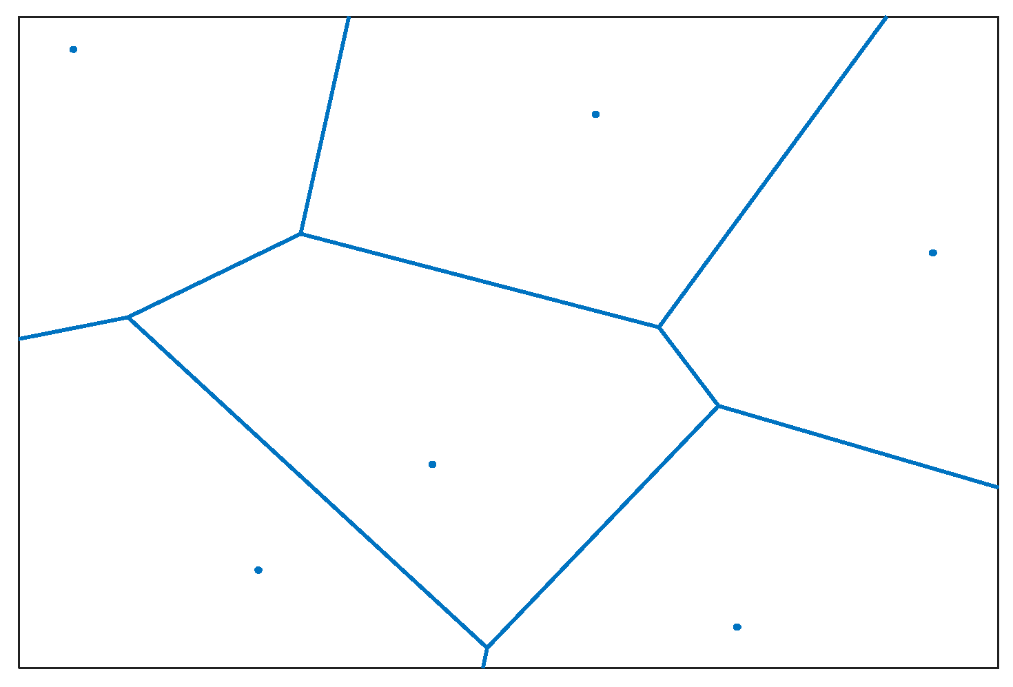
The clustering centers are obtained based on the improved mean shift algorithm, and the clustering centers are used as generating elements using the Voronoi diagram approach to obtain a new sector-planning scheme. A Voronoi diagram [24] is a segmentation of the plane according to the known point set. Given the set of points on the plane , the segmentation of the plane given by is called a Voronoi diagram, with points as generators (or parent points), where is the Euclid distance between points and , and the region is called the Voronoi region of points . Obviously, this region is a set of points on the plane whose distance to the point is smaller than that to other points in the .
The Voronoi diagram is a Voronoi cell-division generation boundary for each generator, that is, the node. The distance from any position in the boundary of the generator to the generator is closer than that to other generators. Figure 5 shows an example of a Voronoi diagram segmentation plane, where the dots represent the generating elements, which in the context of control-area delineation can be the navigation points or mandatory reporting points of an airport, and the fold lines are the Voronoi edges, i.e., the control sector boundaries.
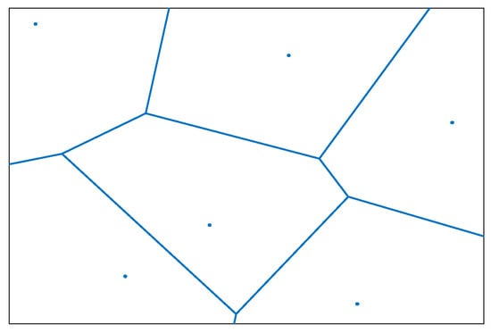
Figure 5.
Voronoi diagram.
5. Validation and Analysis of Sectorization Algorithms
In order to verify the validity of the model and the reasonableness of the sector planning method, the air situation and radar data are obtained through the Air Traffic Operation Management System (ATOM) of Civil Aviation Air Traffic Control Administration (CAAC) and the Xiamen Air Traffic Control Station (Xiamen ATC Station) control simulator for the verification analysis. The Xiamen control area is about 350 km long from east to west and 400 km long from north to south, and there are four sectors in total, and the sector boundaries are recorded and the simulated sectors are drawn using MATLAB to establish the coordinates as shown in Figure 6.
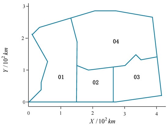
Figure 6.
Simulation of the Xiamen control sector.
5.1. Busy/Idle Time Slots
The flight radar data of Xiamen regional sector from 13 December 2021 to 19 December 2021 were collected as a sample, a total of seven days of operation data, during which there is no strong interference time, and it can be assumed that the data used in this paper are the radar data under normal operation. Record the radar flight data in 10 min intervals, calculate the total nodes, average number of nodes, average point strength, average weighted agglomeration coefficient, network density, and network efficiency of the flight conflict network at each step, and obtain the timeseries of network indicators as shown in Table 3.
Table 3.
Timeseries of network indicators.
The integrated network metrics for intercepts 1–1009 are plotted as a line graph as shown in Figure 7, with the red lines showing the values for the busy and idle time slot divisions.
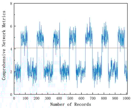
Figure 7.
Changes in consolidated network indicators.
According to the data in Figure 7, ignoring the differences, the comprehensive network indicators have a certain periodicity in the process of time change, and the overall trend is “low plateau period—high plateau period—low plateau period”. Taking the criteria of busy time and idle time as the boundary, it can be divided into the stage of high value of comprehensive network indicators and the stage of low value of network indicators, and roughly deduced that the daily busy time is from 10:00 to 20:00, and the idle time is from 0:00 to 10:00 and from 20:00 to 24:00.
5.2. Sectorization Analysis
According to the busy/idle time segments divided above, the total number of aircraft nodes in the daily busy and idle time segments were recorded at 20 min intervals in the acquired 7-day radar data of Xiamen control area as shown in Table 4.
Table 4.
Total number of aircraft nodes on 7 days.
The EM algorithm is used to cluster the daily busy/idle time period aircraft nodes to find the distribution of daily aircraft regional centers, respectively, and calculate the square of error (SSE) for all the clusters. The case of the 13th busy time period is shown in Figure 8, which can be clearly seen. The time is the optimal time, then all the aircraft nodes of the 13th busy time period will be divided into five categories.
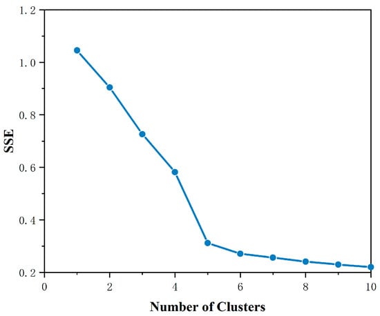
Figure 8.
Error squared graph.
Similarly, the EM algorithm was utilized to cluster the aircraft nodes for the other six date busy/idle time slots to determine the K-values as shown in Table 5.
Table 5.
Number of clustering centers for 7-day busy/idle periods.
The final clustering centers are obtained by clustering the 12,218 aircraft nodes of the original data, and the locations of the clustering centers during busy hours in the coordinate system of Figure 3 are shown in Table 6, with a total of 35 clustering centers during busy hours and 33 clustering centers during idle hours. From the clustering results, it can be observed that the distribution of clustering centers in some busy hours and idle hours are relatively similar, which is due to the influence of approach and departure modes and the location of the navigation station, and most of the flights will be concentrated in the core area of the control sector.
Table 6.
Co-ordinates of cluster centers for busy periods.
For the 35 nodes in the busy time period, the aircraft node-point strength contained in each node is calculated according to Equation (29), and the weight value aa of each node is obtained, and the 35 cluster centers are reduced to 4 using the improved mean shift clustering algorithm described above, and the final cluster center coordinates obtained by clustering are {(113.2, 191.3), (118.4, 64.3), (308.9, 63.1), (288.5, 206.4)}. Based on the MEAN SHIFT segmentation delineation of the sector, the 33 cluster centers of the idle time segments of the same method are clustered similarly to obtain the final cluster center coordinates, {(92.3, 120.4), (209.1, 57.2), (218.0, 214.2), (346.5, 105.8)}, and the cluster centers are used as the generating elements of Voronoi diagrams to obtain the new sector divisions for busy and idle time periods shown in Figure 9.
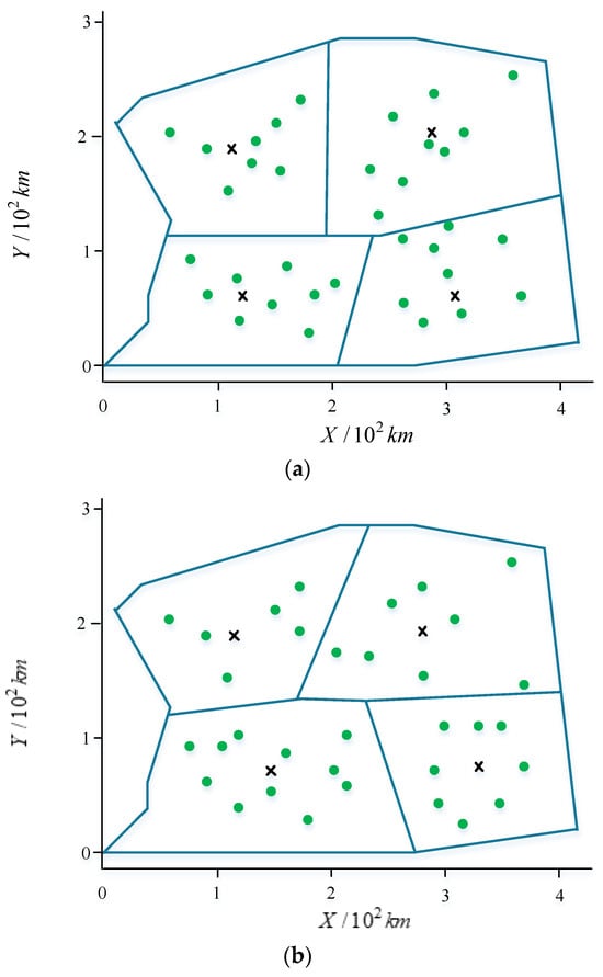
Figure 9.
Final sectorization results. (a) Sectorization during busy hours; (b) Sectorization during idle hours.
5.3. Analysis of Sectorization Results
In order to prove the reasonableness of the delineation of sectors by distinguishing busy/idle time segments, the radar data of any busy and idle time segments are selected to calculate the integrated network indexes of sectors before and after the delineation, and the standard deviation of the integrated network indexes of sectors are compared, and the results obtained are shown in Figure 10.
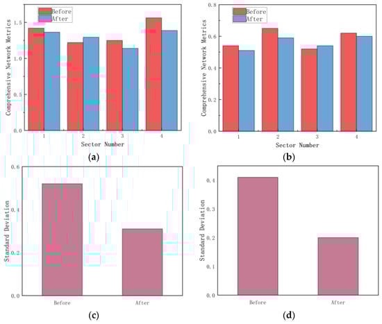
Figure 10.
Comparison of network data before and after delineation. (a) Comprehensive network metrics during busy hours; (b) Comprehensive network metrics during idle hours; (c) Standard deviation of comprehensive network metrics during busy hours; (d) Standard deviation of comprehensive network metrics during idle hours.
As can be seen from Figure 10, whether it is idle time segment or busy time segment, the integrated network index of each sector after the delineation is more balanced relative to the pre-delineation period, and the integrated network index of busy time segment sectors numbered 1~4 is changed from the original {1.421, 1.225, 1.254, 1.562} to the current {1.365, 1.294, 1.140, 1.387}; the integrated network index of each sector standard deviation is reduced by 40.4% compared to the original sector. The integrated network index of idle time segment and busy time segment numbering 1~4 has changed from the original {0.542, 0.654, 0.523, 0.625} to the current {0.517, 0.593, 0.548, 0.601}, and the standard deviation of the integrated network index of each sector has been reduced by 51.2% compared with that of the original sector. After the designation of sectors, the fluctuation of comprehensive network indicators is smaller, the distribution is more balanced, and the flight situation in the sectors has better stability, which is convenient for controllers to maintain stable and efficient working condition.
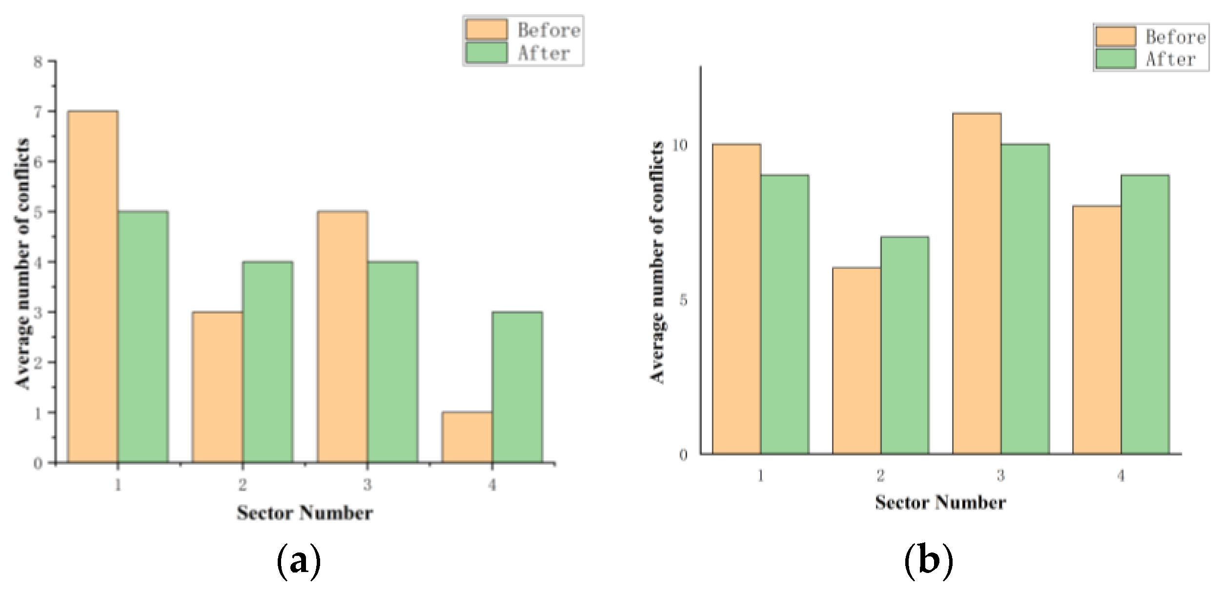
In order to further verify the rationality and effectiveness of the model proposed in this paper, the radar data of the 18:00–20:00 period (busy period) on the 14th and the 07:00–09:00 period (idle period) on the 17th are calculated. The average number of conflicts per unit time and sector before and after sector division is compared, and the results are shown in Figure 11.
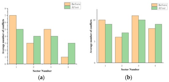
Figure 11.
The average number of conflicts per unit time and sector before and after delineation. (a) The average number of conflicts per unit time and sector during idle hours; (b) The average number of conflicts per unit time and sector during busy hours.
The graph shows that after the model is divided, the average number of conflicts per unit time and sector of each sector in the idle period is changed from {7, 3, 5, 1} to {5, 4, 4, 3}, and the average number of conflicts per unit time and sector of each sector in the busy period is changed from {10, 6, 11, 8} to {9, 7, 10, 9}. The average number of conflicts per unit time and sector can reflect the size of the control load to a certain extent. The results in the figure show that the control load distribution is more uniform after the model is divided, and it will not cause excessive command and deployment pressure to the controller.
6. Conclusions
In this paper, a sector-designation method based on the mean shift algorithm is proposed to obtain different designation schemes for busy and idle time segments based on the clustering of regional flight conditions, and the main innovations are as follows:
(1) The conflict network constructed based on the speed–obstacle relationship between aircraft extends the conflict detection to three dimensions, which can objectively and accurately reflect the flight situation between aircraft;
(2) The radar data of the whole time of recorded flights are selected and an EM clustering algorithm is utilize to cluster and analyze all the aircraft nodes on different dates, which provides extensive data support for sector designation;
(3) The mean shift algorithm searches and clusters according to the distribution of the center position of the node area and the sum of the strength of the aircraft nodes. Combined with the principle of a Voronoi diagram, the busy period and the idle period sector-division schemes are formed, respectively. Compared with other sector division methods, the method proposed in this chapter is based on the original data of the air traffic control radar to explore more comprehensive and objective information in the flight conflict situation.
According to whether the airport is in a busy or idle state, different sector-classification methods are adjusted and planned, so as to facilitate the controller allocating energy more scientifically and reasonably, improving the safety of regional operation, and providing a new reference for current sector-delineation work.
In the process of airspace sector division in idle/busy periods, although the flight conflict situation and air traffic characteristics were comprehensively collected based on historical radar flight data, the selected historical data have certain limitations. In order to improve the universality of the model, the common topological characteristics of radar data should be deeply explored in the next research, and the instance data of multiple control sectors should be used for verification.
Author Contributions
Conceptualization, Y.P. and X.W.; methodology, Y.P.; figure, Y.P. and J.K.; data analysis, Y.P. and Y.M.; writing original draft preparation, Y.P.; writing—review and editing, J.K. and M.W.; supervision, X.W. and M.W.; project administration, M.W. and X.W.; funding acquisition, X.W. All authors have read and agreed to the published version of the manuscript.
Funding
This work was supported in part by the National Science Foundation of China under Grant 71801221.
Data Availability Statement
The data that support the findings of this study are available from the corresponding author, [X.W.], upon reasonable request.
Conflicts of Interest
The authors declare no conflict of interest. The funders had no role in the design of the study; in the collection, analyses, or interpretation of data; in the writing of the manuscript; or in the decision to publish the results.
References
- Zhao, Y.; Wang, M. Theoretical Connotation and Key Science and Technology of Air Traffic Engineering. J. Aeronaut. 2022, 43, 026537. [Google Scholar]
- Delahaye, D.; Alliot, J.M.; Schonenauer, M.; Farges, J.L. Genetic algorithms for partitioning air space. In Proceedings of the Tenth Conference on Artificial Intelligence for Applications, San Antonio, TX, USA, 1–4 March 1994; IEEE: New York, NY, USA, 1994; pp. 291–297. [Google Scholar]
- Yousefi, A.; Denohue, G.L. Temporal and spatial distribution of airspace complexity for air traffic controller workload-based sectorization. In Proceedings of the AIAA 4th Aviation Technology, Integration and Operations (ATIO) Forum, Chicago, IL, USA, 20–22 September 2004; pp. 822–835. [Google Scholar]
- Brinton, C.R.; Pledgie, S. Airspace partitioning using flight clustering and computational Geometry. In Proceedings of the 2008 IEEE/AIAA 27th Digital Avionics Systems Conference, St. Paul, MN, USA, 26–30 October 2008; IEEE/AIAA: New York, NY, USA, 2008. [Google Scholar]
- David, G.; Alliot, J.-M. Optimization of Air Traffic Control Sector Configurations using Tree Search Methods and Genetic Algorithms. In Proceedings of the the 21st Digital Avionics Systems Conference, Irvine, CA, USA, 27–31 October 2002; Volume l, pp. 2A5-1–2A5-8. [Google Scholar]
- Han, S.; Zhang, M.; Huang, W. Methods and computer implementation techniques of control sector optimization. J. Transp. Eng. 2003, 1, 101–104. [Google Scholar]
- Luo, J.; Lu, H. Sector combination optimization based on particle swarm optimization algorithm. Sci. Technol. Eng. 2013, 5, 4130–4133. [Google Scholar]
- Flener, P.; Pearson, J. Propagators and violation functions for geometric and workload constraints arising in airspace sectorisation. arXiv 2014, arXiv:1401.7463. [Google Scholar]
- Sergeeva, M.; Delahaye, D.; Mancel, C. 3D airspace sector design by genetic algorithm. In Proceedings of the 2015 International Conference on Models and Technologies for Intelligent Transportation Systems (MT-ITS), Budapest, Hungary, 3–5 June 2015; IEEE: New York, NY, USA, 2015; pp. 499–506. [Google Scholar]
- Hyo, J. Research on Sectorization under Airspace Complexity Factors. Master’s Thesis, Nanjing University of Aeronautics and Astronautics, Nanjing, China, 2016. [Google Scholar]
- Yan, X. Terminal Airspace Sectorization Method Based on Trajectory Data Mining. Master’s Thesis, Nanjing University of Aeronautics and Astronautics, Nanjing, China, 2020. [Google Scholar]
- Huang, X.; Li, H.N.; Rao, Z.W.; Ding, W. Fracture behavior and self-sharpening mechanisms of polycrystalline cubic boron nitride in grinding based on cohesive element method. Chin. J. Aeronaut. 2019, 32, 2727–2742. [Google Scholar] [CrossRef]
- Legland, D.; Guillon, F.; Devaux, M.F. Parametric mapping of cellular morphology in plant tissue sections by gray level granulometry. Plant Methods 2020, 16, 5872–5881. [Google Scholar] [CrossRef]
- Trandac, H.; Baptiste, P.; Duong, V. Airspace sectorization by constraint programming. In Proceedings of the 1st Conference Recherche, Hanoi, Vietnam, 10–13 February 2023. [Google Scholar]
- Li, J.; Wang, T.; Hwang, I. A spectral clustering based algorithm for dynamic airspace configuration. In Proceedings of the 9th AIAA Aviation Technology, Integration and Operations Conference, Hilton Head, SC, USA, 21–23 September 2009; pp. 21–23. [Google Scholar]
- Soh, S.W. Sectorisation of airspace based on balanced workloads. Aircr. Eng. Aerosp. Technol. 2019, 132, 213–221. [Google Scholar] [CrossRef]
- Lin, F.; Wen, X.; Wu, M.; Heng, Y. Study on sector optimization based on Voronoi diagram and improved K-means. J. Northwestern Polytech. Univ. 2023, 41, 170–179. [Google Scholar] [CrossRef]
- Liang, Y.; He, W.; Zhong, W.; Qian, F. Objective reduction particle swarm optimizer based on maximal information coefficient for many-objective problems. Neurocomputing 2018, 281, 1–11. [Google Scholar] [CrossRef]
- Li, H.W.; Liou, J.J.H. A novel multiple-criteria decision-making-based FMEA model for risk assessment. Appl. Soft Comput. J. 2018, 73, 684–696. [Google Scholar]
- Reshef, D.N.; Reshef, Y.A.; Finucane, H.K.; Grossman, S.R.; McVean, G.; Turnbaugh, P.J.; Lander, E.S.; Mitzenmacher, M.; Sabeti, P.C. Detecting novel associations in large data sets. Science 2011, 80, 1518–1524. [Google Scholar] [CrossRef] [PubMed]
- Rowe, G.; Wright, G. The Delphi technique as a forecastingtool: Issues and analysis. Int. J. Forecast. 2013, 15, 353–375. [Google Scholar] [CrossRef]
- Wang, A.; Zhang, G.; Liu, F. Research and application of EM algorithm. Comput. Technol. Dev. 2009, 19, 108–110. [Google Scholar]
- Zhou, F.; Fan, X.; Ye, Z. Research and application of drifting algorithm. Control. Decis. 2007, 8, 814–847. [Google Scholar]
- Liu, J.; Liu, S. Review of Voronoi diagram application. J. Eng. Graph. 2004, 2, 125–132. [Google Scholar]


Disclaimer/Publisher’s Note: The statements, opinions and data contained in all publications are solely those of the individual author(s) and contributor(s) and not of MDPI and/or the editor(s). MDPI and/or the editor(s) disclaim responsibility for any injury to people or property resulting from any ideas, methods, instructions or products referred to in the content. |
© 2023 by the authors. Licensee MDPI, Basel, Switzerland. This article is an open access article distributed under the terms and conditions of the Creative Commons Attribution (CC BY) license (https://creativecommons.org/licenses/by/4.0/).