Enhanced Frequency-Guided Method with Particle Swarm Optimization for the Phase Recovery of a Single Interferogram

Featured Application

The methods described here can be applied in interferometric measurements of dynamic events that are challenging to analyze using conventional approaches incapable of evaluating a single interferogram with closed fringes.

Abstract

Frequency-guided sequential demodulation (FSD) is a technique used to recover the phase of closed fringe patterns when only a single interferogram is available. FSD is a sequential method that follows simple and intuitive processing steps for interferogram demodulation, guided by the frequency of the fringes. The objective of this work is to apply an optimizer block that feeds from the first stages of the FSD and make feedback in such a manner as to optimize the search for guided frequencies. This approach significantly reduces demodulation errors, especially when dealing with high-frequency fringe patterns. The results of using the FSD with and without optimizers are compared. The optimizers used are the Harmonic Search Optimization (HSO) as well as the Particle Swarm Optimization (PSO). Results show that FSD with PSO delivers better results compared with other methods here analyzed.

1. Introduction

Interference is a fundamental optical phenomenon that emerges when two or more waves, whether mechanical or electromagnetic, overlap within the same spatial plane. The scientific discipline tasked with measuring and harnessing this interference is known as interferometry. Interferometry plays a pivotal role in various domains, ranging from the precise assessment of aberrations, deformations, and flatness to addressing challenges posed by disturbances and temperature gradients [1].

The methodologies that are usually preferred to demodulated interferograms are the phase-shift algorithms and the Fourier method for single linear carrier fringe patterns [2]. However, these techniques often struggle in the case of rapidly changing events because the phase difference between consecutive interferograms is not a constant. In this situation, a large linear carrier interferogram can be recorded but at the cost of a reduced dynamic range of the phase that can be measured. Attempts to record a fringe pattern in the described situation would lead to infringing the sampling theorem. A solution to measure a dynamic event with a high dynamic phase range is to analyze a single interferogram with closed fringes. A unique interferogram with closed fringes can be examined to recover the phase information associated with the physical phenomena being measured. The measurement accuracy from a unique closed fringe pattern is thus closely dependent on the phase distribution of the interferogram being measured.

Several phase demodulation methods from a single fringe pattern have been proposed. Each one of the proposed solutions has strengths and drawbacks. There are methods that use different computational strategies, such as the combination of genetic algorithms and parametric methods [3,4,5]; soft computing techniques applied to Zernike polynomials [6]; a combination of genetic algorithms and frequency-guided sequential demodulation [7]; combined harmony search optimization and frequency-guided sequential demodulation [1]; demodulate directly with Particle Swarm Optimization [8]; unwrapping of phase maps with sign changes [9]; demodulation with symmetric wavefront and tilt [10]; two-dimensional regularized phase-tracking technique [11]; different techniques of deep learning [12,13]; convolutional neural network [14]; and Lissajous ellipse fitting [15], among others.

While each of these methods demonstrates efficacy in specific contexts and scenarios, no universal approach exists capable of reliably extracting phase information from any given interferogram. Some of the mentioned methods have a slow convergence rate, require a specific path determination method to avoid critical points, and need a large training set of known solutions to the demodulation problem, besides a high computational complexity. Rather, these techniques are optimized for particular characteristics of fringe patterns, thus limiting their applicability in broader contexts. All techniques are susceptible to be improved.

In particular, the optical phase demodulation has been expressed as an optimization problem, where computational intelligence algorithms can be applied to find the best phase solution that matches with the closed fringe patterns called interferogram. In 2007 Kemao and Soon proposed a frequency-guided sequential demodulation (FSD) technique suggesting a single fringe pattern demodulation by estimating the local frequencies of the interferogram, where the phase sign determination is guided by the frequency or fringe density [16].

Harmony search optimization (HSO) is a soft computing technique inspired by the observation of musical composition to search for perfect harmony and was introduced in 2001 by Geem et al. [17]. In 1995, Kennedy and Eberhart proposed an evolutionary algorithm that consists of the optimization of the data using a cloud of particles in order to model social problems; this algorithm is known as Particle Swarm Optimization (PSO) [18]. Given advances in optimization algorithms, they can support techniques in different areas of science. Both optimization techniques have found their way into several areas of scientific knowledge as diverse as engineering [19,20,21], math optimization [22,23] and optical applications [8,24,25], among other applications [26].

Recently, the FSD has been combined with an evolutionary algorithm known as HSO, with good results. Here, we proposed to implement the FSD approach with another evolutionary algorithm, known as PSO. It is found that the proposed combination scheme FSD-PSO delivers more robust results than FSD or FSD-HSO techniques, particularly when the interference pattern possesses high-frequency fringes and also with a complex distribution. In the following section, the FSD principle is explained, as well as the combination of the optimization algorithms (PSO and HSO) with the FSD algorithm, and the sign change determination process is explained, too. Then, the simulation results are presented, and, finally, the discussions and conclusions are declared.

2. Materials and Methods

Optical metrology is a discipline whose aim is to carry out measurements of objects by applying engineering to optical phenomena such as interference, diffraction, and polarization, among others. Devices such as interferometers, diffractometers and polarimeters are used to accomplish those measurements. Particularly, interferometers use light as a measurement unit and, unlike other disciplinary techniques in science, they have the advantage of being non-invasive measurement methods.

2.1. Interferometry

Interferometry studies the interaction of two or more wavefronts, where one of them has undergone a modification by a feature of the object being measured [27]. It should be mentioned that the fewer the interfering wavefronts, the higher the measurement resolution will tend since the more wavefronts interact, the greater the number of harmonics will be generated in the Fourier spectrum, and at the time of demodulation it will be confusing to interpret which of the interfering wavefronts belongs to each harmonic. Phase demodulation is the more important task in optical interferometry measurements because the physical quantity to be measured is directly related to the phase [1].

The fringe pattern intensity produced by a division amplitude interferometer as Michelson, Twyman-Green, Fizeau, etc. can be modeled by

$$I_{\eta }\left(x,y\right)=a_{\eta }\left(x,y\right)+b\left(x,y\right)\cos \left[\phi \left(x,y\right)\right].$$

(1)

where $I_{\eta }(x,y)$ is the interference fringe pattern intensity unprocessed, $a_{\eta }(x,y)$ is the background intensity with a possible noise term $\eta (x,y)$ added to it, $b(x,y)$ is the amplitude modulation, $\phi (x,y)$ is the phase term and $(x,y)$ is the spatial coordinates of the physical quantity under testing.

2.2. Frequency-Guided Sequential Demodulation

The FSD demodulation method was developed by Kemao and Soon, as explained in the introductory section, to demodulate closed fringe patterns with a single interferogram. The sequential algorithm FSD is explained below in the following 6 steps (for a more detailed explanation the reader is encouraged to consult references [16,28]):

1.

The pre-processing image (denoise filtering), which consists of attenuating possible noise $\eta (x,y)$ of the interferogram $I_{\eta }(x,y)$, taking care that the interference fringes are not distorted. With this process, $\eta (x,y)$ is suppressed from $a_n(x,y)$ to obtain the filtered background intensity $a(x,y)$ of the filtered interferogram $I(x,y)$, which is

$$I\left(x,y\right)=a\left(x,y\right)+b\left(x,y\right)\cos \left(\phi \left(x,y\right)\right).$$

(2)

2.

To cancel the background intensity $a(x,y)$ and the modulation amplitude $b(x,y)$ coefficients, a normalization procedure has to be carried out considering that both terms vary slowly compared to the cosine of the phase. Usually, high-pass filters can be used to remove background intensity, but there are regions of $b\left(x,y\right)\cos \left(\phi \left(x, y\right)\right)=f\left(x,y\right)$ that can also present low frequencies, especially when the phase is flat, so information can be lost with this type of filtering. Another more efficient way to eliminate the coefficient $a$ is using the Empirical Mode Decomposition (EMD), which decomposes the signal in many harmonics and a residual noise term, as shown in [29].

It continues with the elimination of the modulation coefficient $b(x,y)$; for this, it is suggested to use the Hilbert transform to obtain

$$H\left\{f\left(x,y\right)\right\}=-b\left(x,y\right)\sin \left(\phi \left(x, y\right)\right),$$

(3)

and with which the term $b(x,y)$ can be eliminated in two ways: the first one obtaining the magnitude to find $b(x,y)$, which is

$$b\left(x,y\right)=\sqrt{{\left(H\left\{f\left(x,y\right)\right\}\right)}^2+{\left(f\left(x,y\right)\right)}^2},$$

(4)

and then divide by $f(x,y)$; and the second one is applying a cosine function to the $\arctan (-H\left\{f\left(x,y\right)\right\}/f\left(x,y\right))$ term. Therefore, the normalized interferogram becomes

$$I_n\left(x,y\right)=\cos \left(\phi \left(x,y\right)\right).$$

(5)

3.

The direct extraction of the phase ${\widehat{\phi }}_{wa}(x,y)$, which is carried out by applying the arccosine function to the interferogram. This stage of the phase is used to calculate the intermediate frequencies ${\widehat{\omega }}_{xa}(u,v)$ and ${\widehat{\omega }}_{ya}(u,v)$, where $(u,v)$ are the local coordinates of the window being processed. Once the optimization process is complete, the final frequencies ${\widehat{\omega }}_a(u,v)$ are available, which guarantees that the optimization algorithm found a global minimum. Then,

$${\widehat{\phi }}_{wa}\left(x,y\right)=\arccos \left(I_n\left(x,y\right)\right), \in \left[0,\pi \right].$$

(6)

4.

The extraction of the local phase ${\tilde{\phi }}_a(x,y)$ is considered linear in a small window of the interferogram. The energy function is defined as the square of the difference of the normalized interferogram $I_n(x,y)$ and the virtual interferogram $\tilde{I}(x,y)$ is calculated. Then, the local frequencies are allocated inside the minimized energy function as

$$\widehat{P}\left(u,v\right)={\left[{\widehat{\omega }}_{xa}\left(u,v\right),{\widehat{\omega }}_{ya}\left(u,v\right)\right]}^T.$$

(7)

5.

The extraction of the estimated frequency by the optimization method, which is a vector of two calculated values of the pixel under study.

6.

Eliminate the ambiguity error. Finding a function for the determination of the sign $s$, which depends on the final frequencies and the local phase.

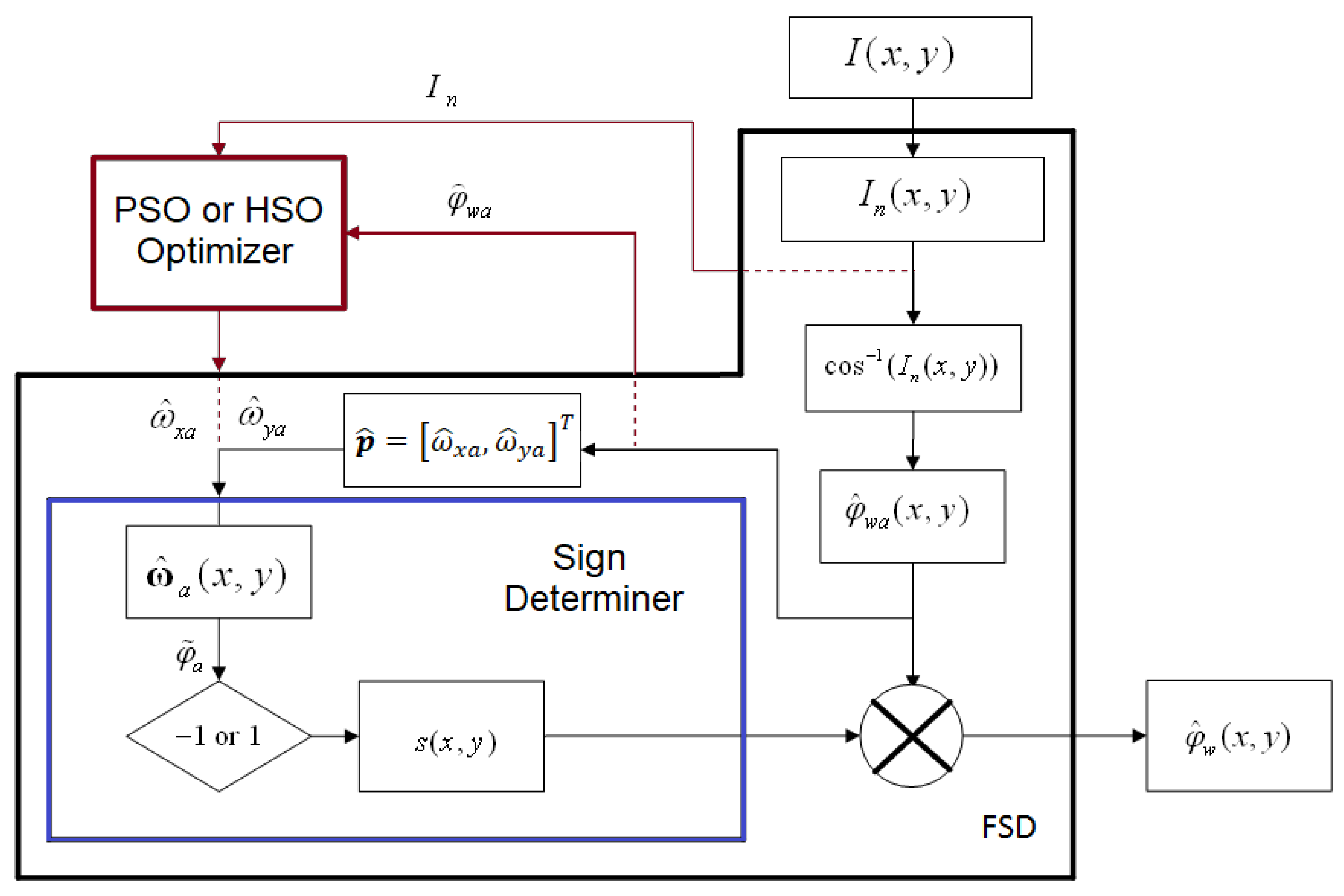
To optimize the FSD algorithm, both evolutionary algorithms, the PSO (proposed optimizer) as well as the HSO (optimizer used in [1]), were applied. The proposed method is summarized in the flowchart shown in Figure 1, where the user can choose among FSD (in black), FSD-HSO or FSD-PSO (both in red). The input parameters to the optimization block are the normalized interferogram $I_n\left(x,y\right)$, as well as the local phase ${\widehat{\phi }}_{wa}\left(x,y\right)$, which are obtained from the first steps of the FSD. The optimizer finds the best values of the intermediate frequencies ${\widehat{\omega }}_{xa}\left(u,v\right)$ and ${\widehat{\omega }}_{ya}\left(u,v\right)$, that are fed to the sign-determining block of the FSD. At the algorithm’s end, the wrapped phase ${\widehat{\phi }}_w(x,y)$ is obtained, which depends on the method used: FSD, FSD-HSO or FSD-PSO. To obtain the unwrapped phase ${\widehat{\phi }}_u\left(x,y\right)$, standard unwrapping algorithms can be used. The unwrapping algorithm used in this work was least squares [30].

The operation of the PSO optimizer within the optimization block of Figure 1 is detailed below. The position of a set of particles is randomly initialized. Then, it is necessary to iteratively update the $(x,y)$ positions of the particles in the swarm to find the best positions through a cost function; that is:

$$cost\left(u,v\right)={\left[I_n\left(u,v\right)-\cos \left(w_x\left(u-x\right)+w_y\left(v-y\right)+{\widehat{\phi }}_{wa}\left(x,y\right)\right)\right]}^2,$$

(8)

where $w_x$ and $w_y$ are the current positions in $(x,y)$, respectively. In addition, a random update of the particles is carried out, iteratively comparing the current position versus the best position within the swarm. At the end of the interactions, the best $(x,y)$ positions found will correspond to the intermediate frequencies ${\widehat{\omega }}_{xa}$ and ${\widehat{\omega }}_{ya}$, respectively. The PSO algorithm applied to FSD is as follows [18,19]:

1.

Inputs: normalized interferogram $I_n$ and local enveloped phase ${\widehat{\phi }}_{wa}$.

2.

The PSO parameters are established.

3.

The position of the particles is initialized randomly.

• The best-known position of the particle swarm is updated by means of the cost function.

4.

The speed of the particles is initialized, randomly.

• The speed of the particles is updated based on their best position with respect to the current position;
• The best position within the swarm is updated.

5.

The intermediate frequencies ${\widehat{\omega }}_{xa}$ and ${\widehat{\omega }}_{ya}$ are found based on the best positions found within the swarm, during the total number of valid iterations.

The implementation details of the algorithm PSO were particle number 80, inertia weight 0.5, cognitive coefficient 0.3, social coefficient 0.2 and iterations 20. Similarly, for the HSO algorithm were harmony search solutions 100, harmony memory considering rate 0.9, pitch adjusting rate 0.2 and iterations 100. In both algorithms, the following parameters will be the same: dimensions of problem 2, lower and upper limits [−1, 1], neighborhood region for energy function 11 and optimal cost value 0.25, as well as the iterations mentioned before were applied, as long as the cost function was less than 2.5. The operation of the FSD-HSO algorithm can be consulted in reference [1].

3. Results

In order to test the three algorithms (FSD, FSD-HSO and FSD-PSO), synthetic interferograms were implemented, which contained Gaussian functions in strategic positions of the interferogram. The normalized interferogram $I_n\left(x,y\right)$ now reads

$$I_n\left(x,y\right)=\cos \left[{\rho }_1\phi \left(x,y\right)\right],$$

(9)

where ${\rho }_1$ controls the general amplitude of the entire phase, and $\phi \left(x,y\right)$ is the sum of several Gaussians $g_{xx}$,

$$\phi \left(x,y\right)=A·g_{nw}+B·g_{ne}+C·g_{sw}+D·g_{se}+E·g_c.$$

(10)

The Gaussians $g_{xx}$ programmed in each synthetic interferogram were placed at the northeast ($g_{ne}$), northwest ($g_{nw}$), southeast ($g_{se}$), southwest ($g_{sw}$) and central ($g_c$) positions. Parameters A to D are used to activate each of the Gaussians individually. Internally, the Gaussians can be written relative to their position xx or yy = nw, ne, sw, se or c, respectively; that is

$$g_{xx}=\exp \left({-\rho }_2\left[F_{xx}{\left(x-N_{xx}\right)}^2+F_{yy}{\left(y-N_{yy}\right)}^2\right]\right),$$

(11)

where the parameters $F_{xx}$ and $F_{yy}$ individually controls the width of the Gaussian at $x$ and $y$ positions, respectively, and the parameter ${\rho }_2$ determines the width of each Gaussian generally in $(x,y)$ positions. To control the positions of each of the Gaussians, the parameters $N_{xx}$ and $N_{yy}$ are used. The synthetic wrapped phase is calculated as

$${\phi }_w\left(x,y\right)=\arctan \left[\frac{\sin \left({\rho }_1\phi \left(x,y\right)\right)}{\cos \left({\rho }_1\phi \left(x,y\right)\right)}\right].$$

(12)

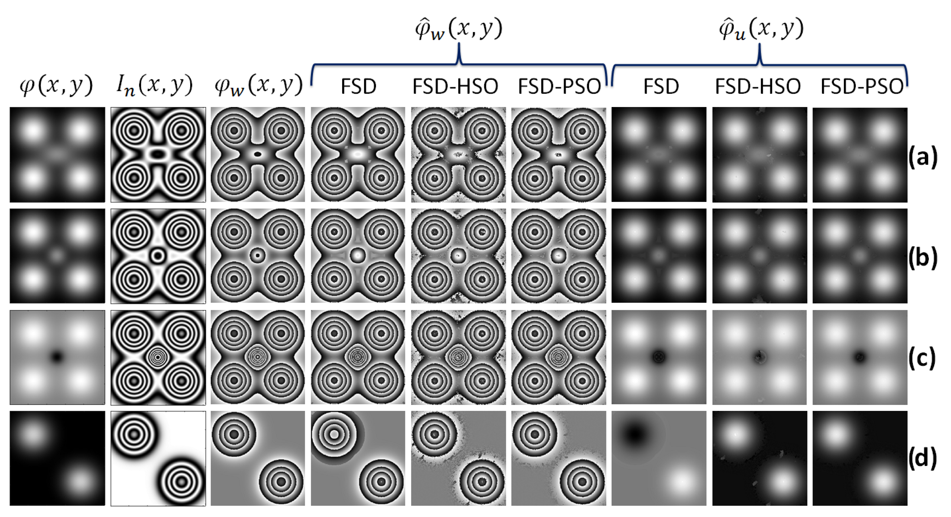
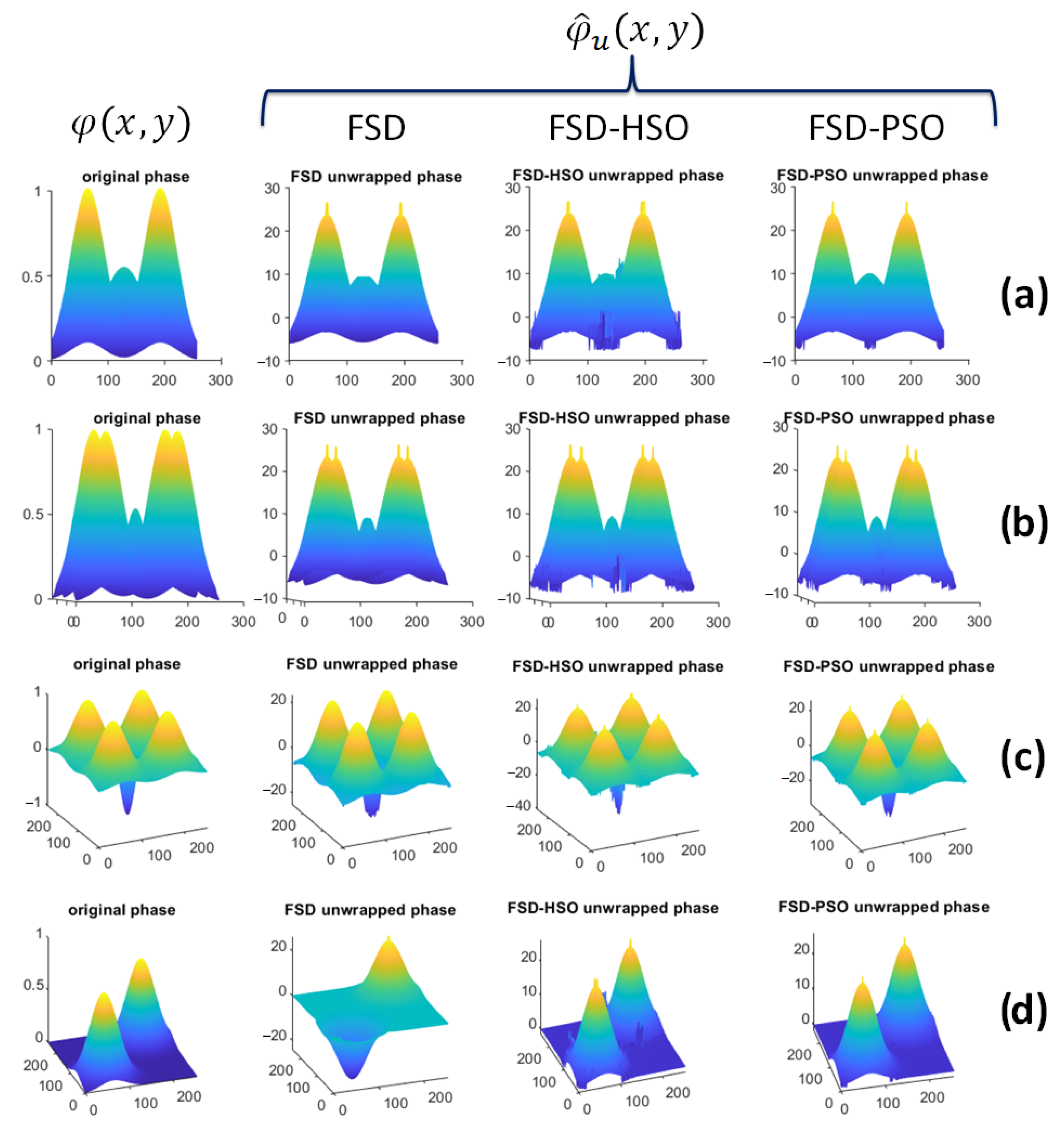
In Figure 2, the results with different types of synthetic interferograms are shown: in rows (a–b), five positive Gaussian examples are presented; in row (c), an example with four positive Gaussians and a negative one is depicted; and in the final row (d), two Gaussian interferograms are seen. Figure 3 shows the 3D phases representations of the interferograms shown in Figure 2, in order to observe the differences between the original phase $\phi \left(x,y\right)$ with the unwrapped phases calculated ${\widehat{\phi }}_u\left(x,y\right)$ with the FSD and FSD-HSO algorithms, as well as the proposed algorithm FSD-PSO. The fixed parameters in all synthetic interferograms were: $N=256$, ${\rho }_1=-30$, ${\rho }_2=1/1800$, as well as the size of the interferograms was N × N.

To calculate the original phase $\phi \left(x,y\right)$, Gaussians presented in Figure 2 and Figure 3 rows (a)–(c), the following parameters were used: $a\left(x,y\right)=0$, $b\left(x,y\right)=1$, $A=1$, $B=1$, $C=1$, $D=1$, $F_{xx}=1$ and $F_{yy}=1$ are fixed in $g_{ne}$, $g_{nw}$, $g_{se}$ and $g_{sw}$, but $g_c$ acts as adjustable Gaussian. In these cases, the $g_c$ parameters change as follows: in row (a) $E=0.5$, $F_{xx}=2$ and $F_{yy}=1$; in row (b) $E=0.5$, $F_{xx}=3$ and $F_{yy}=3$; and in row (c) $E=-1$, $F_{xx}=5$ and $F_{yy}=5$. In row (d), only two Gaussian functions are shown, with $A=0.8$, $B=0$, $C=0$, $D=0.8$ and $E=0$, as well as their respective thickness parameters are $F_{xx}=1$ and $F_{yy}=1$.

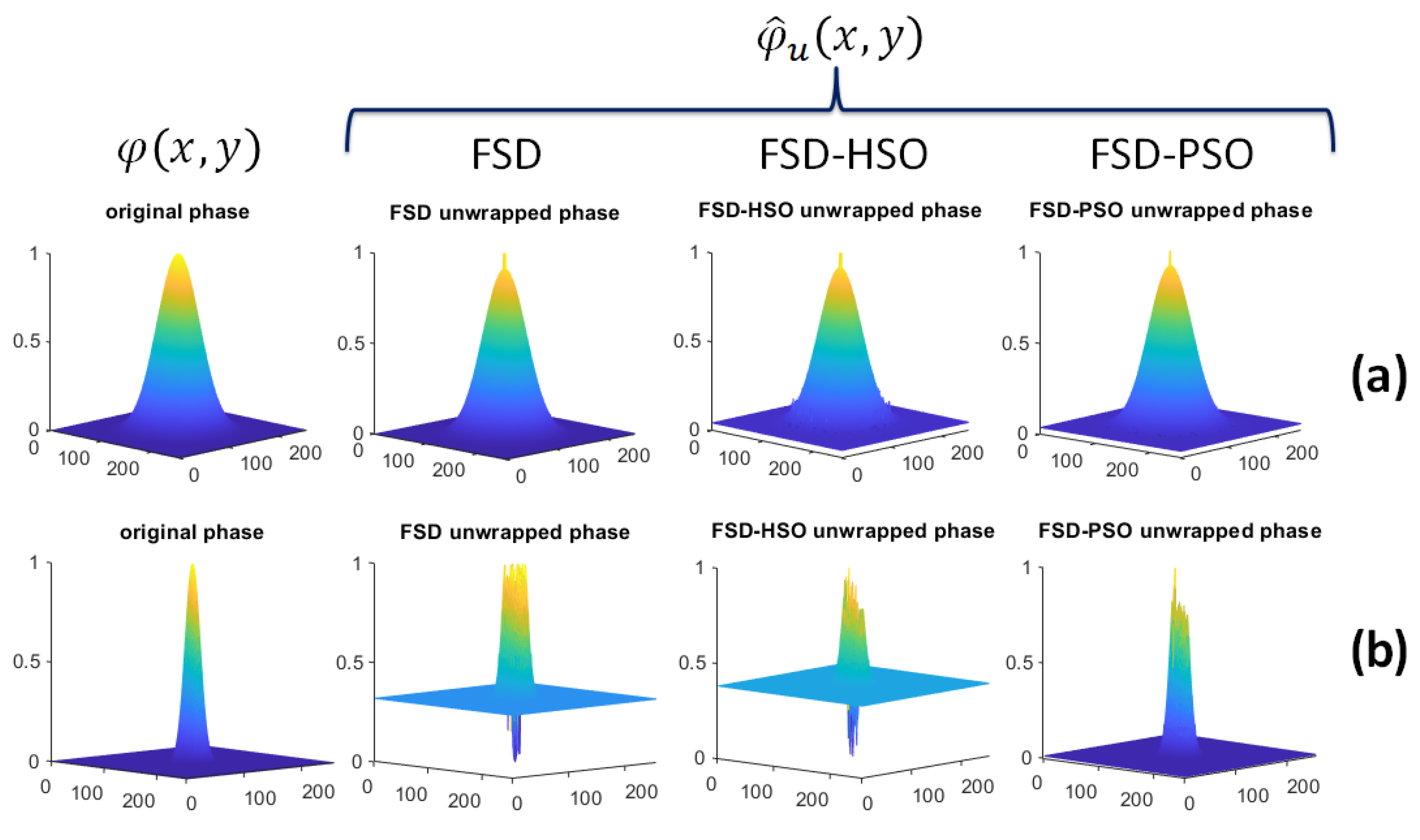
A set of interferograms with a single Gaussian function with varying width and amplitude were calculated in order to test the response of the considered methods with respect to the fringe frequency. In Figure 4 it is shown the two cases of the gaussian functions, $F_{xx}=F_{yy}=1$ and 10. A 3D view of the recovered phases is shown in Figure 5, where in row (a) all the methods had success, in row (b) details of the behavior of the different methods in high-frequency interferograms are shown, where it can be observed the Gaussian peaks distortion. In addition to $F_{xx}$ and $F_{yy}$, the remaining parameters used to obtain the interferograms and phases of Figure 4 and Figure 5 were:$A=0$, $B=0$, $C=0$, $D=0$ and $E=1$. The interpretation of the results is given in the next section.

4. Discussion

The results of our study, which evaluated the performance of three algorithms (FSD, FSD-HSO, and FSD-PSO) using synthetic interferograms, provide valuable insights into the capabilities and limitations of these demodulation techniques.

4.1. Performance with Synthetic Interferograms

In our investigation, we employed synthetic interferograms that incorporated strategically positioned Gaussian functions. The normalized interferogram $I_n(x,y)$ was defined, allowing us to control the overall amplitude of the phase ${\rho }_1$ and introduce several Gaussian components (A to E) into the phase $\phi \left(x,y\right)$. These Gaussian components were strategically placed in the northeast, northwest, southeast, southwest, and central positions within the interferograms. The parameters $F_{xx}$ and $F_{yy}$ were employed to regulate the width of these Gaussians, while ${\rho }_1$ determined their overall scale. Additionally, the positions of these Gaussians were manipulated using $N_{xx}$ and $N_{yy}$.

Evaluation of Demodulation Methods: In Figure 2, we presented the results obtained from different synthetic interferograms, categorizing them into various scenarios:

• Figure 2a,b showcase two examples with five positive Gaussians;
• Figure 2c features an example with four positive Gaussians and one negative Gaussian;
• Figure 2d depicts an interferogram with two Gaussian components.

For a more comprehensive analysis, 3D representations of the phases of these interferograms were provided in Figure 3, allowing us to compare the original phase $\phi \left(x,y\right)$ with the unwrapped phases computed using the FSD, FSD-HSO, and FSD-PSO algorithms.

Fringe Frequency Variation Testing: To assess the methods’ performance concerning fringe frequency, we generated interferograms with single Gaussian functions that varied in width and amplitude. These experiments are depicted in Figure 4, where we presented two cases: $F_{xx}=F_{yy}=1$ and $F_{xx}=F_{yy}=10$. Subsequently, we examined 3D views of the recovered phases in Figure 5.

4.2. Key Observations and Insights

Our study yielded several significant findings and observations:

(1)

Method Robustness: The results indicate that the FSD technique performs adequately with low-frequency interferograms, successfully recovering the phase in most scenarios. However, some challenges arise, particularly in cases with central peaks and scenarios with multiple Gaussians, Figure 2a and Figure 2d, respectively.

(2)

FSD-HSO Performance: FSD-HSO exhibits improved performance compared to the standard FSD method, yielding better results and fewer artifacts. Nevertheless, some regions in the interferograms still present noticeable artifacts, affecting the quality of the demodulated phase.

(3)

Superiority of FSD-PSO: FSD-PSO emerges as the standout performer among the three algorithms. It consistently produces more accurate and faithful results, with reduced artifacts and a closer resemblance to the original phase.

(4)

Frequency Sensitivity: The experiments with varying Gaussian widths and amplitudes provide insights into frequency sensitivity. Both FSD and FSD-HSO exhibit limitations as fringe frequencies increase, with notable distortions observed in Gaussian peaks. FSD-PSO demonstrates a more stable response, but it also exhibits some sensitivity to higher frequencies.

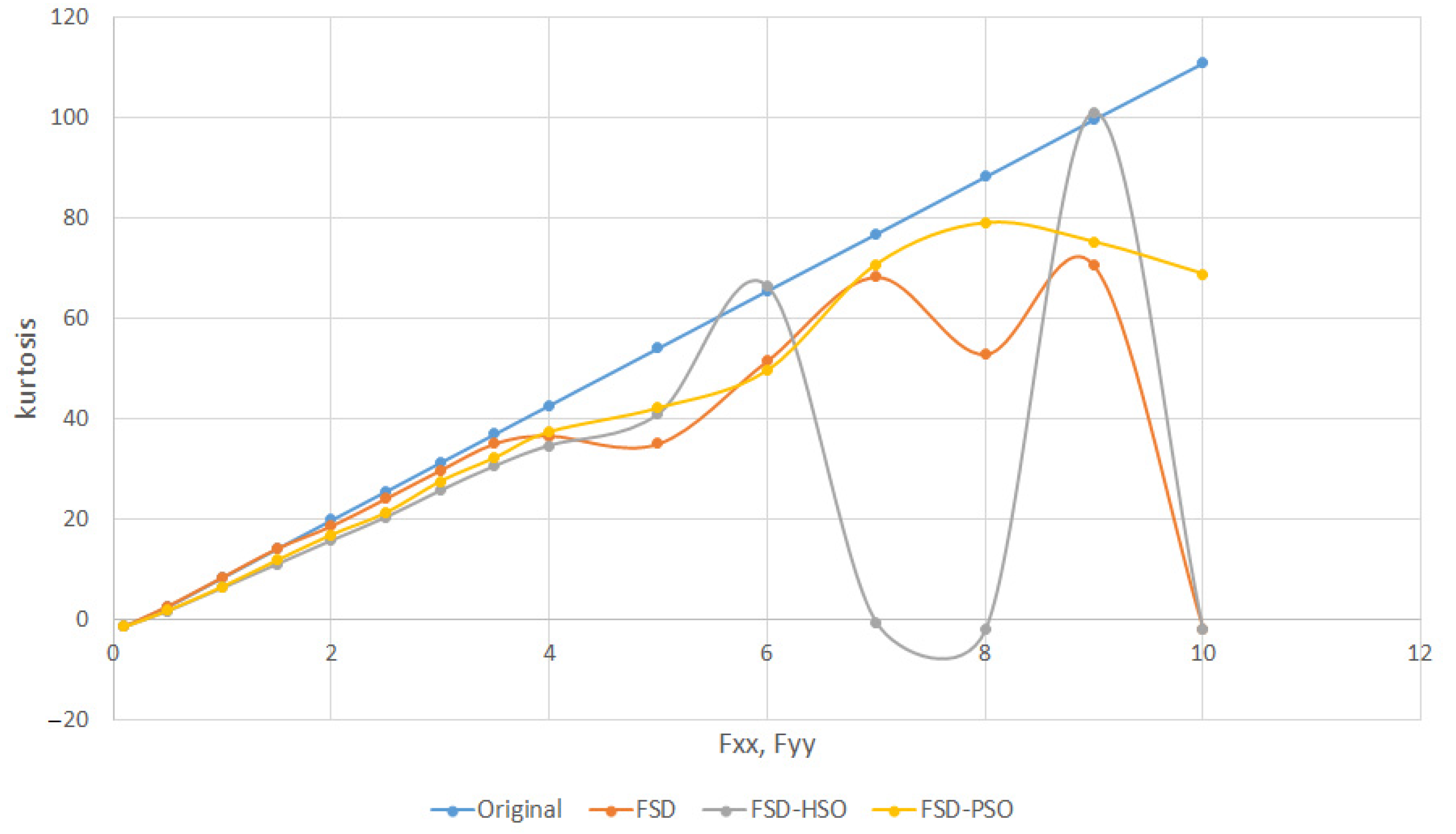
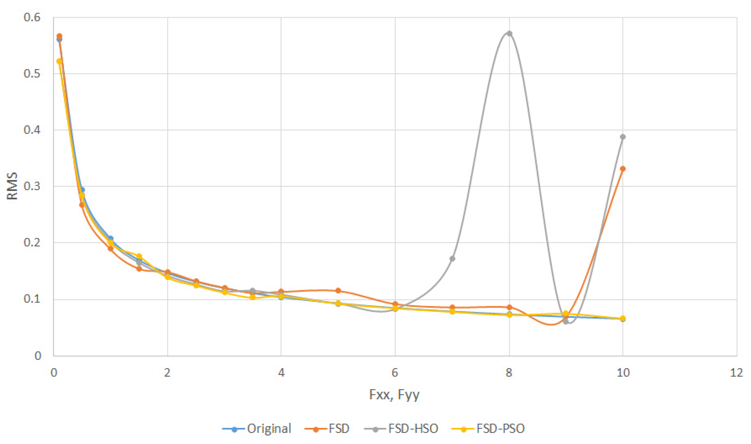
4.3. Quantitative Assessment

To quantitatively assess the algorithms’ performance, we introduced kurtosis and root mean square (RMS) parameters. Kurtosis values provided insights into the recovered Gaussian function widths, with positive values indicating a slim, high-profile curve and negative values suggesting a flattened profile [31]. Notably:

• FSD began to falter when $F_{xx}$ exceeded 7;
• FSD-HSO exhibited a diminishing response for $F_{xx}$ values greater than 6;
• FSD-PSO showcased a more favorable performance, deteriorating only slightly when $F_{xx}$ approached higher values, as shown in Figure 6.

Similarly, RMS values illustrated divergence from the original phase as fringe frequencies increased:

• FSD-HSO began to diverge when $F_{xx}$ exceeded 6;
• FSD exhibited divergence when $F_{xx}$ surpassed 8.

FSD-PSO showed remarkable consistency with the original phase, diverging only significantly higher values, as shown in Figure 7.

5. Conclusions

In this study, we conducted a comprehensive evaluation of three demodulation algorithms, namely FSD, FSD-HSO, and FSD-PSO, using synthetic interferograms. Our aim was to gain a deeper understanding of the capabilities and limitations of these techniques in the context of optical interferometry.

Through the use of synthetic interferograms, we were able to control various parameters, such as the amplitude, position, and width of Gaussian components within the interferograms. These numerical experiments allowed us to assess the performance of the demodulation methods across different scenarios, including those with positive and negative Gaussians and varying fringe frequencies.

This study yielded several important findings and insights:

• Method Robustness: The standard FSD technique exhibited satisfactory performance, particularly with low-frequency interferograms, where it successfully recovered the phase in most cases. However, challenges arose in scenarios involving central peaks and multiple Gaussians, as observed in Figure 2a and Figure 2d.
• FSD-HSO Performance: FSD-HSO demonstrated improved performance compared to the standard FSD method. It produced better results with fewer artifacts. Nevertheless, some regions in the interferograms still exhibited noticeable artifacts, impacting the quality of the demodulated phase.
• Superiority of FSD-PSO: FSD-PSO emerged as the standout performer among the three algorithms. It consistently delivered more accurate and faithful results, with reduced artifacts and a closer resemblance to the original phase.
• Frequency Sensitivity: Our experiments with varying Gaussian widths and amplitudes provided insights into the frequency sensitivity of the methods. Both FSD and FSD-HSO exhibited limitations as fringe frequencies increased, leading to distortions in Gaussian peaks. FSD-PSO demonstrated a more stable response, although it also exhibited some sensitivity to higher frequencies.

To quantitatively evaluate the algorithms’ performance, we introduced kurtosis and RMS parameters. These parameters offered insights into the recovery of Gaussian function widths and divergence from the original phase as fringe frequencies increased.

Our study highlights the strengths of FSD-PSO as a superior demodulation technique. One important consideration about the use of optimizers with the FSD technique is that adds computational complexity and also increases the demodulation time. It is essential to acknowledge other limitations and potential drawbacks:

• Computational Resources: FSD-PSO, being computationally intensive, may require substantial computational resources for real-time applications. This could be a limiting factor in scenarios where real-time results are essential.
• Parameter Tuning: The optimal performance of FSD-PSO may rely on fine-tuning numerous algorithm parameters. Achieving these optimal settings can be a non-trivial task and may require expertise.
• Sensitivity to Extremely High Frequencies: While FSD-PSO demonstrates greater stability in high-frequency scenarios compared to its counterparts, it may still exhibit sensitivity to extremely high fringe frequencies, necessitating careful consideration of application-specific requirements.

In conclusion, our research contributes to a better understanding of the demodulation capabilities of FSD and its optimized variants FSD-HSO and FSD-PSO. FSD-PSO, in particular, stands out as a promising approach for accurate phase recovery from interferograms. However, researchers and practitioners should be mindful of the computational demands and parameter-tuning requirements associated with this technique. Further research is warranted to explore its practical applicability in real-world optical interferometry scenarios and address the identified limitations.

References

- Rodriguez-Marmolejo, U.H.; Mora-Gonzalez, M.; Muñoz-Maciel, J.; Ramirez-delreal, T.A. FSD-HSO Optimization Algorithm for Closed Fringes Interferogram Demodulation. Math. Probl. Eng. 2016, 2016, 1576735. [Google Scholar] [CrossRef]
- Malacara, D.; Servin, M.; Malacara, Z. Interferogram Analysis for Optical Testing, 2nd ed.; CRC Press: Boca Raton, FL, USA, 2018; pp. 399–454. [Google Scholar]
- Cuevas, F.J.; Sossa-Azuela, J.H.; Servin, M. A parametric method applied to phase recovery from a fringe pattern based on a genetic algorithm. Opt. Commun. 2002, 203, 213–223. [Google Scholar] [CrossRef]
- Cuevas, F.J.; Mendoza, F.; Servin, M.; Sossa-Azuela, J.H. Window fringe pattern demodulation by multi-functional fitting using a genetic algorithm. Opt. Commun. 2006, 261, 231–239. [Google Scholar] [CrossRef]
- Toledo, L.E.; Cuevas, F.J. Optical metrology by fringe processing on independent windows using a genetic algorithm. Exp. Mech. 2008, 48, 559–569. [Google Scholar] [CrossRef]
- Mancilla Espinosa, L.E.; Carpio Valadez, J.M.; Cuevas, F.J. Demodulation of interferograms of closed fringes by Zernike polynomials using a technique of soft computing. Eng. Lett. 2007, 15, 99–104. [Google Scholar]
- Rodriguez-Marmolejo, U.H.; Ramirez-Delreal, T.A.; Muñoz-Maciel, J.; Mora-Gonzalez, M. Combination of genetic algorithms and FSD applied to fringe pattern demodulation. In Proceedings of the Volume 9600, Image Reconstruction from Incomplete Data VIII, San Diego, CA, USA, 11–12 August 2015; SPIE: Philadelphia, PA, USA, 2015. [Google Scholar]
- Jiménez, J.; Sossa, H.; Cuevas, F.; Gómez, L. Demodulation of interferograms based on particle swarm optimization. Polibits 2012, 45, 83–91. [Google Scholar] [CrossRef]
- Muñoz-Maciel, J.; Casillas-Rodríguez, F.J.; Mora-Gonzalez, M.; Peña-Lecona, F.G.; Duran-Ramírez, V.M.; Gómez-Rosas, G. Phase recovery from a single interferogram with closed fringes by phase unwrapping. Appl. Opt. 2011, 50, 22–27. [Google Scholar] [CrossRef] [PubMed]
- Muñoz-Maciel, J.; Duran-Ramírez, V.M.; Mora-Gonzalez, M.; Casillas-Rodriguez, F.J.; Peña-Lecona, F.G. Demodulation of a single closed-fringe interferogram with symmetric wavefront and tilt. Opt. Commun. 2019, 436, 168–173. [Google Scholar] [CrossRef]
- Servin, M.; Marroquin, J.L.; Cuevas, F.J. Demodulation of a single interferogram by use of a two-dimensional regularized phase-tracking technique. Appl. Opt. 1997, 36, 4540–4548. [Google Scholar] [CrossRef]
- Kando, D.; Tomioka, S.; Miyamoto, N.; Ueda, R. Phase Extraction from Single Interferogram Including Closed-Fringe Using Deep Learning. Appl. Sci. 2019, 9, 3529. [Google Scholar] [CrossRef]
- Zuo, C.; Qian, J.; Feng, S.; Yin, W.; Li, Y.; Fan, P.; Han, J.; Qian, K.; Chen, Q. Deep learning in optical metrology: A review. Light-Sci. Appl. 2022, 11, 39. [Google Scholar] [CrossRef] [PubMed]
- Liu, X.; Yang, Z.; Dou, J.; Liu, Z. Fast demodulation of single-shot interferogram via convolutional neural network. Opt. Commun. 2021, 487, 126813. [Google Scholar] [CrossRef]
- Liu, F.; Kuang, Y.; Wu, Y.; Chen, X.; Zhang, R. Phase retrieval from single interferogram without carrier using Lissajous ellipse fitting technology. Sci. Rep. 2023, 13, 9917. [Google Scholar] [CrossRef]
- Kemao, Q.; Soon, S.H. Sequential demodulation of a single fringe pattern guided by local frequencies. Opt. Lett. 2007, 32, 127–129. [Google Scholar] [CrossRef] [PubMed]
- Geem, Z.W.; Kim, J.H.; Loganathan, G.V. A new heuristic optimization algorithm: Harmony search. Simulation 2001, 76, 60–68. [Google Scholar] [CrossRef]
- Kennedy, J.; Eberhart, R. Particle swarm optimization. In Proceedings of the ICNN’95—International Conference on Neural Networks, Perth, WA, Australia, 27 November–1 December 1995. [Google Scholar]
- Gad, A.G. Particle Swarm Optimization Algorithm and Its Applications: A Systematic Review. Arch. Comput. Methods Eng. 2022, 29, 2531–2561. [Google Scholar] [CrossRef]
- Ingram, G.; Zhang, T. Overview of applications and developments in the harmony search algorithm. In Music-Inspired Harmony Search Algorithm: Theory and Applications; Geem, Z.W., Ed.; Springer: New York, NY, USA, 2009; Volume 191, pp. 15–37. [Google Scholar]
- Gao, X.Z.; Govindasamy, V.; Xu, H.; Wang, X.; Zenger, K. Harmony search method: Theory and applications. Comput. Intell. Neurosci. 2015, 2015, 258491. [Google Scholar] [CrossRef]
- Deng, F.; Tuo, S.; Yong, L.; Zhou, T. Construction example for algebra system using harmony search algorithm. Math. Probl. Eng. 2015, 2015, 836925. [Google Scholar] [CrossRef]
- Li, G.; Wang, Q. A cooperative harmony search algorithm for function optimization. Math. Probl. Eng. 2014, 2014, 587820. [Google Scholar] [CrossRef]
- Menke, C. Application of particle swarm optimization to the automatic design of optical systems. In Proceedings of the Optical Design and Engineering VII, 106901A, Frankfurt, Germany, 5 June 2018; SPIE: Philadelphia, PA, USA, 2018. [Google Scholar]
- Yue, W.; Jin, G.; Yang, X. Adaptive Particle Swarm Optimization for Automatic Design of Common Aperture Optical System. Photonics 2022, 9, 807. [Google Scholar] [CrossRef]
- Manjarres, D.; Landa-Torres, I.; Gil-Lopez, S.; Del Ser, J.; Bilbao, M.N.; Salcedo-Sanz, S.; Geem, Z.W. A survey on applications of the harmony search algorithm. Eng. Appl. Artif. Intell. 2013, 26, 1818–1831. [Google Scholar] [CrossRef]
- Hecht, E. Optics, 5th ed.; Addison-Wesley: San Francisco, CA, USA, 2017; pp. 398–456. [Google Scholar]
- Kemao, Q. Windowed Fringe Pattern Analysis; SPIE Press: Bellingham, WA, USA, 2013; pp. 200–207. [Google Scholar]
- Huang, N.E.; Shen, Z.; Long, S.R.; Wu, M.C.; Shih, H.H.; Zheng, Q.; Yen, N.; Tung, C.C.; Liu, H.H. The empirical mode decomposition and the Hilbert spectrum for nonlinear and non-stationary time series analysis. Proc. R. Soc. Lond. Ser. A Math. Phys. Eng. Sci. 1998, 454, 903–995. [Google Scholar] [CrossRef]
- Ghiglia, D.C.; Romero, L. Robust two-dimensional weighted and unweighted phase unwrapping that uses fast transforms and iterative methods. J. Opt. Soc. Am. A 1994, 11, 107–117. [Google Scholar] [CrossRef]
- Pratt, W.K. Digital Image Processing: PIKS Scientific Inside, 4th ed.; John Wiley & Sons, Inc.: New York, NY, USA, 2007; pp. 535–577. [Google Scholar]