Modeling an Optimal Environmentally Friendly Energy-Saving Flexible Workshop

Abstract

From the perspective of energy efficiency and environmental sustainability, the scheduling problem in a flexible workshop with the utilization of automated guided vehicles (AGVs) was investigated for material transportation. Addressing the dual-constrained integrated scheduling challenge involving machining machines and AGVs, a scheduling optimization model was established with makespan, workshop energy consumption, and processing quality as the optimization objectives. To effectively solve this model, an enhanced whale optimization algorithm (IWOA) was proposed. Specifically, nonlinear convergence factors, adaptive inertia weights, and improved helix positions were introduced into the standard whale optimization algorithm to update the model. Furthermore, a loss function was constructed based on fuzzy membership theory to obtain the optimal compromise solution of the multi-objective model. The research results indicate that: (1) The IWOA obtained the optimal solutions on benchmark instances MK01, MK02, MK04, MK07, and MK08; (2) The IWOA outperformed the WOA(1), WOA(2), WOA-LEDE, and NSGA-II algorithms in the two instances provided in this paper, demonstrating strong robustness of the model; (3) Although the multi-objective model constructed in this paper could not surpass the single-objective optimal solution in individual objectives, it achieved compensation in other objectives, effectively balancing the trade-offs among the makespan, workshop energy consumption, and processing quality of the three objectives. This research offers an effective practical approach to address green flexible workshop scheduling with AGV transportation.

1. Introduction

1.1. Background and Motivation

The Fourth Industrial Revolution (intelligent era) has opened the curtain, and the production mode of the manufacturing industry has begun to shift to automation and intelligence [1]. The transformation and innovation of the manufacturing production mode have led to the traditional large-scale standardized manufacturing mode being replaced by the multi-variety, small batch, short cycle, and personalized manufacturing mode, which also puts forward higher requirements for workshop production flexibility and processes [2]. Therefore, it is an urgent need for manufacturing enterprises to solve the scheduling problem before processing or assembly to optimize their manufacturing resource allocation strategy and improve the utilization rate of manufacturing resources. It should be emphasized that shop floor scheduling has become a bottleneck and key problem faced by manufacturing enterprises [3,4]. A reasonable flexible shop floor scheduling scheme is the key to improving efficiency, reducing costs and allocating resources reasonably for manufacturing enterprises.

In recent years, manufacturing enterprises have actively promoted the concept of advanced intelligent manufacturing. In order to realize the transformation from a traditional manufacturing shop to intelligent shop, many manufacturing enterprises have introduced automated logistics equipment such as automatic guided vehicles (AGVs). This has made the traditional optimal allocation of manufacturing tasks, machines, and personnel gradually expand to the integrated optimization of multi-types of manufacturing resources [5]. In the actual job shop, different path choices of AGVs cause different time consumption. It will also affect the processing time, scheduling planning, and completion time of the entire production task. Therefore, flexible shop floor integrated scheduling with an AGV has gradually become one of the key research problems in the field of production scheduling optimization.

In flexible job shop scheduling (FJS), AGVs are used for material transportation, which breaks the constraint of machine uniqueness in traditional shop floor production. In the flexible job shop scheduling problem (FJSP), the number of alternative AGV sets to transport materials to any machine meeting the production requirements for processing in the alternative machine sets, so that the workshop production scheduling problem can be flexibly scheduled according to the different actual needs. FJSP includes operations such as machine loading and unloading, production activity programming, machine planning and allocation, AGV allocation, and AGV path selection [6,7,8], which also makes the optimal allocation of production resources more complex. Therefore, FJSP using AGV transportation is an extension of FSSP and the traditional shop scheduling problem, which is a more complex and difficult NP-hard problem [9]. It is well-known that accurate algorithms can find it difficult to obtain excellent exact solutions of NP-hard problems in limited time, and their solving speed and accuracy are far less than that of intelligent optimization algorithms [10,11,12,13]. Furthermore, the FJSP may necessitate the simultaneous consideration of multiple objectives, some of which might exhibit conflicting interests. This not only leads to an expansive search space, but also makes it challenging to attain optimality within a short timeframe. Therefore, it is very challenging to solve the flexible job-shop scheduling problem with large-scale and multi-objectives.

1.2. Literature Review

It can be found from recent studies that the intelligent optimization algorithm is the most common method to solve a FJSP that adopts an AGV for material transportation, and the near-optimal or optimal solution of the scheduling problem can be obtained through continuous update and iteration [14]. Zheng et al. [15] developed a mixed integer linear programming model with the goal of minimizing the manufacturing period and proposed a heuristic algorithm solution model based on tabu search. Umar et al. [16] took the minimization of delay cost and the minimization of makespan as objective functions and solved the model with genetic algorithm to solve the integrated scheduling problem of processing equipment and an AGV in FMS. Saidmehrabad et al. [17] discussed the path planning problem of an AGV in a flexible job shop. Taking the makespan as the optimization objective, they proposed a two-stage ant colony algorithm to first solve the allocation and path selection problems of an AGV. Sanchesi et al. [18] constructed a planning model with the goal of shortening the manufacturing cycle to the maximum extent under the minimum running time and adopted an adaptive genetic algorithm to solve the optimal scheduling scheme. Nageswararao [19] proposed a meta-heuristic gravity search algorithm to solve the scheduling problems of processing equipment and AGVs in a job shop. The model constructed aimed at minimizing the makespan, completing assigned tasks faster, and solving system resources. Fazlollahtabar [20] designed a network optimization algorithm to solve the problems of AGV scheduling and path planning as well as the scheduling problems of production equipment. Taking the minimum waiting time as the delay penalty objective letter, he established a mathematical model suitable for the control of the minimum cost according to the delay cost. Li et al. [21] constructed a flexible shop scheduling model aimed at minimizing the AGV buffer waiting time and total driving distance and proposed an improved harmony search algorithm to solve the mathematical model. Lyu et al. [22] considered the optimal number of AGVs, the shortest transportation time, and path planning, and proposed an improved genetic algorithm to solve the integrated scheduling problem of AGVS and processing equipment in a flexible manufacturing system with the makespan as the optimization objective. Zhu et al. [23] established a flexible job-shop scheduling model aiming at minimizing the makespan, studied flexible job-shop scheduling with AGVs, and proposed an improved genetic algorithm solution model. Lei et al. [24] proposed a meme algorithm combining waiting time to solve FJSP to minimize the makespan. As can be seen from the above FJSP regarding the use of an AGV for material transportation, the scheduling objective of most workshops has only been the completion time measurement, without considering the factors related to energy saving and emissions reduction.

In recent years, environmental problems have become increasingly prominent, reducing carbon emissions and building a resource-saving and environmentally friendly society has become the consensus of all countries worldwide. As an energy-intensive field, manufacturing consumes nearly one third of the world’s energy [25,26]. The study of energy saving shop scheduling is of great significance to the sustainable development of the industry [27,28]. Therefore, the questions of how to reduce the energy consumption of the workshop as much as possible and realize reasonable scheduling of processing equipment and AGVs under the condition of ensuring normal operation of the workshop and minimizing production time have become research hotspots. Liu et al. [29] studied a green multi-objective logistics system problem where the objective was to simultaneously minimize the makespan and energy consumption, and they proposed a new multi-population co-evolutionary algorithm to solve it. Jiang et al. [30] considered a green job-shop scheduling problem and constructed a planning model aimed at minimizing the sum of energy consumption cost and completion time cost of the workshop, and designed an optimized discrete whale to solve the model. Yao et al. [31] developed an optimization model aiming at minimizing the AGV energy consumption and production cost, and proposed a nonlinear mixed integer programming genetic algorithm. Jiang et al. [32] established a green shop scheduling optimization model aimed at minimizing the total energy consumption and proposed an improved African Buffalo optimization algorithm to solve this problem. In order to balance production and green and sustainable development, Peng et al. [33] constructed a multi-objective flexible job-shop scheduling model with processing time, energy consumption, and noise minimization as the objectives under the dual resource constraints of human and machine, and developed a hybrid discrete multi-objective imperial competitive algorithm based on the model. Afsar et al. [34] proposed a new enhanced meme algorithm to solve a job-shop scheduling problem with dual objectives, namely, minimum machine energy consumption and minimum makespan. Chen et al. [35] explored the energy consumption of AGVs in manufacturing environments and investigated the AGV energy-efficient scheduling problem with customer satisfaction in flexible manufacturing systems.

The whale optimization algorithm (WOA) is a new meta-heuristic algorithm proposed by Mirjalili et al. in 2016 [36]. It has the advantages of a simple search strategy, few parameters, and strong search ability. Compared with other classical algorithms (genetic, particle swarm optimization, ant colony, etc.), the main uniqueness of the WOA algorithm is that it can maintain a good exploration and development relationship by self-adjusting some parameters in the iterative process, and it has been widely used in solving a variety of optimization problems [37,38,39,40]. In terms of shop scheduling, Luan et al. [41] proposed a new and improved whale optimization algorithm to solve the scheduling scheme of a flexible shop scheduling problem. They improved the convergence factor of the whale algorithm and introduced the inertia weight. Jiang et al. [42] introduced a nonlinear convergence factor and mutation operation of scheduling rules on the basis of a standard WOA algorithm. Liu et al. [43] proposed a hybrid whale swarm optimization algorithm (WOA-LFDE) based on Levy flight to solve the problem of job-shop scheduling optimization, and improved the search ability and convergence speed of the algorithm by changing the search strategy and flight mode.

To sum up, existing studies have made many achievements in the model construction and algorithm solving of a FJSP. The summary is as follows:

(1) In a FJSP that adopts an AGV for material transportation, few existing studies have put forward restrictions on the number of AGVs. In addition, the path optimization of processing equipment allocation and AGV scheduling scheme is considered more, and the objective function constructed is mostly a single objective programming model, that is, the makespan is minimum, without considering the shop energy consumption and processing quality.

(2) In the existing green FJSP, scholars take the completion time and energy consumption of processing equipment into consideration when modeling, but there are few studies on the joint scheduling of processing equipment and AGVs from the perspective of green scheduling. Therefore, the energy consumption in the existing green FJSP only considers the energy consumption of processing equipment, while ignoring the energy consumption of AGV scheduling.

(3) In the optimization algorithm of the FJSP solution, many improved algorithms based on genetic algorithm, tabu search algorithm, ant colony algorithm, and other classical intelligent algorithms have been applied, but the local search performance and convergence speed of the above algorithms still need to be further improved.

(4) According to the literature [41,42,43], the optimization algorithm based on WOA can effectively solve the shop scheduling problem. The experimental results show that the improved algorithm based on the WOA algorithm is better than the improved algorithm based on classical algorithm (such as genetic algorithm, particle swarm optimization algorithm, ant colony algorithm, tabu search algorithm, etc.), and also better than the improved algorithm based on the memetic algorithm, teaching and learning optimization algorithm, and biogeographic-based optimization algorithm.

1.3. Contribution

According to the above, an improved algorithm (IWOA) based on WOA was proposed to solve the green FJSP with AGV transportation. It is important to note that, like other meta-heuristic algorithms, WOA also has the disadvantages of easily falling into local optimum and premature convergence [36]. The global search ability of WOA has certain randomness and static clustering behavior, and its ability to jump out of the local optimum is limited, which leads to the tendency to fall into the local optimum in the process of solving the target problem. Furthermore, in the exploration stage of the WOA, the operation of learning from random individuals is blind, and there is no effective information exchange among groups, which affects the convergence speed of the algorithm. This problem is particularly prominent in large-scale complex optimization problems. To alleviate such problems, three techniques are used to improve the overall performance of the WOA.

(1) A nonlinear convergence factor is introduced. The convergence decreases nonlinearly with the increase in the number of evolutionary iterations to ensure that the total group of whales moves with a large stride in the initial stage and a small stride in the later stage. It enhances the exploration ability of the algorithm and improves the convergence speed of the algorithm.

(2) Nonlinear adaptive inertia weights were added to the algorithm to balance the local search and global search of the algorithm and avoid the algorithm falling into local optimization.

(3) The screw position update model was improved to increase the diversity of the total population and retain more high-quality individuals to improve the solution quality. In addition, according to the characteristics of this model, a loss function based on fuzzy membership was constructed in order to obtain the optimal compromise solution of the multi-objective model.

Considering the processing characteristics of the flexible workshop, that is, several operations can be processed on different machines, and the processing time, the processing energy consumption and processing quality of the same operation must be different for different machines. Therefore, it is not sufficient to take the completion time as the basis of shop scheduling without considering the energy consumption and processing quality of the shop.

In short, on the premise of ensuring product quality and the stability of the production system, it is more practical to optimize the resource allocation strategy, improve the resource utilization rate, reduce the production energy consumption, and explore the green FJSP with the dual constraints of processing equipment and transportation AGV, which is closer to the real situation of modern workshops. The main contributions of this paper are as follows:

(1) A multi-objective optimization scheduling model of a green flexible job shop was established to maximize the machining quality and minimize the makespan and energy consumption. In this paper, the energy consumption of the processing equipment and AGV scheduling were considered comprehensively.

(2) An improved whale optimization algorithm (IWOA) was proposed and the fitness function of the algorithm constructed.

(3) Based on fuzzy membership degree theory, the satisfaction function (loss function) was constructed to transform multiple objectives into a single objective. At the same time, several feasible scheduling schemes were provided to the decision-makers, so that the decision-makers could choose the optimal scheduling scheme according to the actual situation.

In summary, the purpose of this research was to address the scheduling problem in a flexible workshop by establishing a multi-objective optimization model aimed at maximizing the processing quality while minimizing the makespan and workshop energy consumption. This study aimed to optimize resource allocation strategies, reduce energy consumption, and provide decision-makers with various feasible scheduling solutions to achieve an environmentally friendly production system.

The rest of this paper is organized as follows. In Section 2, a multi-objective optimization model of green FJSP is presented. In Section 3, an IWOA is designed to solve the optimization problem. The proposed model and algorithm are evaluated in Section 4. Conclusions and future work are provided in Section 5.

2. Multi-Objective Optimization Model of Green FJSP

2.1. Problem Description

A green FJSP that uses AGVs for material transportation can be described as follows: there are i independent jobs processed on m_k machines, n AGVs are responsible for moving jobs between machines, and each AGV can transport jobs between any machine and storage area. The AGV initially docks at the unprocessed job storage area m₀. When the scheduling task occurs, the AGV will transport the job to the corresponding machine according to the processing sequence of the job and unload the job. If no new scheduling task is received at this time, the AGV will be on standby in situ. If a new scheduling task is received, the AGV goes to the task point for material transportation, and the above process is repeated until all the jobs are processed and transported to the finished product storage area m_k+1 by the AGV.

In this paper, the FJSP was decomposed into three sub-problems: process sequencing, AGV selection and allocation, and machine selection. The optimization objective was to minimize the makespan and energy consumption in the workshop and maximize the processing quality. To simplify the problem, the following assumptions were made:

(1) Both the machines and AGVs were assumed to be free of faults and fully powered for efficient dispatching.

(2) All production equipment and AGVs were operational at zero hour and could only be completely shut down after all operations assigned to them had been completed.

(3) The driving speed of all AGVs was constant, and the driving time only depended on the driving distance.

(4) The machine needed to be set up before processing different operations.

(5) AGV idle time incurred no energy consumption.

(6) Machines had unlimited storage space for waiting jobs to be further processed.

2.2. Mathematical Model

The parameter notations involved in the model, and their definitions are given in

Table 1. Description of the notations.

Notations	Definition	Notations	Definition
i	Set of jobs, i = {1, 2, 3, ..., I}	tijkk’v	Transport time of operation Oij from machine mk to machine mk’ by AGV wv
j	Set of operations, j = {1, 2, 3, ..., Ji}	qijk	Processing quality of operation Oij on machine mk
Ji	Number of operations for job i	αijk	Energy consumption of operation Oij on machine mk
M	Set of processing machines, M = {m1, m2, ..., mk}	μk	Energy consumption of machine mk in idle state
W	Set of AGV, W = {w1, w2, ..., wv}	σk	Setup energy consumption coefficient of machine mk
Osijk	Starting time of operation Oij on machine mk	τv	Energy consumption of AGV wv driving
Oijk	Processing time of operation Oij on machine mk	Mijk	Setup time of machine mk for operation Oij
Oeijk	Completion time of operation Oij on machine mk	L	A big positive number
tsijv	Starting time of AGV v transport operation Oij	xijk	If operation Oij is to be processed on machine mk, xijk = 1; otherwise, xijk = 0
teijv	Completion time of AGV wv transport operation Oij	yijv	If operation Oij is transported by AGV wv, yijv = 1; otherwise, yijv = 0
tij0kv	Transport time of operation Oij from unprocessed job storage area M0 to machine mk by AGV wv	xiji’j’k	If Oij is processed on machine mk prior to Oi’j’, xiji’j’k = 1; otherwise, xiji’j’k = 0
tijkk+1v	Transport time of operation Oij from machine mk to finished job storage area Mk+1 by AGV wv	yiji’j’v	If Oij is transported by AGV wv prior to Oi’j’, yiji’j’v = 1; otherwise, yiji’j’v = 0

.

The objective function of the green FJSP of AGVs and machine integrated scheduling is as follows:

(1)

The makespan Z1 is the shortest, that is, the maximum processing time of the last operation of the job is the minimum.

(2)

The total energy consumption of processing machines and AGV transportation Z2 is the smallest. The total energy consumption of machines includes three parts: the total energy consumption of machine operation, the total energy consumption of idle machines, and the total energy consumption of machine setting.

(3)

The processing quality Z3 of a certain operation on a machine is reflected by the qualified rates of the operation on the machine, that is, the processing quality is expressed by the qualified rates. A job includes n operations, and we regarded the average quality of all operations as the processing quality of the job.

$$Z1=\min \left[\max O_{ijk}^e\right]$$

(1)

$$Z2=\min \left[\begin{array}{l}{\displaystyle \sum _{i\in I}{\displaystyle \sum _{j\in J}{\displaystyle \sum _{k\in K}{O}_{ijk}{x}_{ijk}{\alpha }_{ijk}}}}+{\displaystyle \sum _{k\in K}\left(\max \left\{O_{ijk}^e\right\}-{\displaystyle \sum _{i\in I}{\displaystyle \sum _{j\in J}{O}_{ijk}{x}_{ijk}}}\right){\mu }_k}\\ +{\displaystyle \sum _{i\in I}{\displaystyle \sum _{j\in J}{\displaystyle \sum _{i\prime \in I}{\displaystyle \sum _{j\prime \in J}{\displaystyle \sum _{k\in K}{M}_{ijk}{x}_{ijik}{\sigma }_k}}}}}+{\displaystyle \sum _{v\in V}\left(\begin{array}{l}{\displaystyle \sum _{i\in I}{\displaystyle \sum _{j=1}{\displaystyle \sum _{k\in K}{t}_{ij0kv}{x}_{ijk}}}}\\ +{\displaystyle \sum _{i\in I}{\displaystyle \sum _{j\in J}{\displaystyle \sum _{k\in K}{\displaystyle \sum _{k\prime \in K}{t}_{ijkk\prime v}}}{x}_{ijk}{x}_{ijk\prime }}}\\ +{\displaystyle \sum _{i\in I}{\displaystyle \sum _{j=J_i}{\displaystyle \sum _{k\in K}{t}_{i{J}_{i}kk+1v}}{x}_{i{J}_{i}k}}}\end{array}\right)}{\tau }_v\end{array}\right]$$

(2)

$$Z3=\min \frac{{\displaystyle \sum _{k\in K}{\displaystyle \sum _{i\in I}{\displaystyle \sum _{j\in J}{q}_{ijk}{x}_{ijk}}}}}{{\displaystyle \sum _{i\in I}{J}_i}}$$

(3)

According to the actual demand of job-shop scheduling, constraints are set. This paper mainly considered the dual resource constraints of the processing machine and AGV.

• Constraints between operations and machines.

  (1)

  A operation can only be processed on one machine:

  $${\displaystyle \sum _{k\in K}{x}_{ijk}}\le 1$$

  (4)

  (2)

  Machine processing sequence constraint, a machine can only process the next process after the previous process is completed and the machine setting is completed:

  $$O_{ijk}^e+M_{i\prime j\prime k}\le O_{i\prime j\prime k}^s+L\left(1-x_{iji\prime j\prime k}\right)$$

  (5)

  (3)

  Each job includes multiple operations, and the operations have sequential constraints. The next operation can only be processed after the previous operation of the same job is completed:

  $$O_{ijk}^e\le O_{ij+1k\prime }^s$$

  (6)

  (4)

  After the machine starts processing an operation, it is not allowed to be interrupted:

  $$O_{ijk}^e=O_{ijk}^s+{\displaystyle \sum _{k\in K}{O}_{ijk}^{}}{x}_{ijk}$$

  (7)

2.

Constraints between operations and AGVs.

(1)

Only one AGV can be selected for a transportation task:

$${\displaystyle \sum _{v\in V}{y}_{ijv}}\le 1$$

(8)

(2)

The order of AGV transportation is restricted. The same AGV cannot transport multiple jobs at the same time, and the jobs are transported in the order of job processing:

$$t_{ijv}^e\le t_{i\prime j\prime v}^s+L\left(1-y_{iji\prime j\prime v}\right)$$

(9)

(3)

The end time of the AGV to complete the task transportation is equal to the start transportation time plus the transportation time:

$$\{\begin{array}{l}{t}_{i1v}^e=t_{i1v}^s+{\displaystyle \sum _{v\in V}{\displaystyle \sum _{k\in K}{t}_{i10kv}}}{x}_{i1k}{y}_{i1v},j=1\\ t_{ijv}^e=t_{ijv}^s+{\displaystyle \sum _{v\in V}{\displaystyle \sum _{k\in K}{\displaystyle \sum _{k\prime \in K}{t}_{ijkk\prime v}}}}{x}_{ijk}{x}_{ijk\prime }{y}_{ijv},j>1\end{array}$$

(10)

3.

Constraints between AGVs and machines.

(1)

The AGV transports the job to the machine, and the operation can only be processed when the machine is idle:

$$\max \left(t_{{}_{ijv}}^e,O_{i\prime j\prime k}^e\right)\le O_{ijk}^s+L\left(1-x_{i\prime j\prime ijk}\right)$$

(11)

(2)

The AGV transports the job from the unprocessed job storage area to the machine that processes the first operation:

$$t_{{}_{ijv}}^s+{\displaystyle \sum _{k\in K}{\displaystyle \sum _{v\in V}{t}_{ij0kv}}}{x}_{ijk}{y}_{ijv}\le O_{{}_{ijk}}^s,j=1$$

(12)

(3)

The AGV transports the job from one machine to another for processing of the next operation of the job:

$$O_{ijk}^e+{\displaystyle \sum _{v\in V}{\displaystyle \sum _{k\in K}{\displaystyle \sum _{k\prime \in K}{t}_{ij+1kk\prime v}}}}{x}_{ijk}{x}_{ij+1k\prime }{y}_{ij+1v}\le O_{ij+1k\prime }^s$$

(13)

(4)

After the last operation of the job is completed, the AGV transports it to the finished job storage area:

$$O_{i{J}_{i}k}^s+{\displaystyle \sum _{k\in K}{O}_{i{J}_{i}k}^{}}{x}_{i{J}_{i}k}^{}+{\displaystyle \sum _{k\in K}{\displaystyle \sum _{v\in V}{t}_{i{J}_{i}kk+1v}}}\le O_{i{J}_{i}k}^e$$

(14)

3. An Improved Whale Optimization Algorithm (IWOA) for Solving the Green FJSP

The solution algorithm of the dual resource integrated scheduling model for processing machines and distribution AGVs in a flexible job shop is designed in this section.

Based on the above content, FJSP is a typical NP-hard problem, so we tried to use an improved whale optimization algorithm to solve the problem. First, the optimization principle of the whale optimization algorithm (WOA) was described. Second, the encoding and decoding methods of the scheduling scheme were designed. Then, an improved whale optimization algorithm (IWOA) was designed, and a nonlinear decline strategy, adaptive weight strategy, and improved screw position update strategy were proposed to improve the overall performance of the algorithm. Finally, a logical framework combining the whale optimization algorithm was designed to solve the scheduling problem in this paper.

3.1. Whale Optimization Algorithm (WOA)

Mirjalili and Lewis [36] proposed a whale optimization algorithm based on the shrinking encircling mechanism and spiraling updating mechanism according to the behavior characteristics of whales catching prey through bubble net behavior. In the algorithm, the definition is:

(1) The number of whales involved in hunting is N.

(2) The search space is d-dimensional.

(3) $x_i=(x_{}^1,x_{}^2,\dots ,x_{}^d),i=1,2,\dots ,N$ represents the position of the i-th whale in d-dimensional space.

(4) $x^{*}=(x_{}^{1*},x_{}^{2*},\dots ,x_{}^{d*})$ represents the position of prey in space d.

(5) The location of the target prey corresponds to the global optimal solution of the optimization problem.

(1) Shrinking encircling

Since there is no prior knowledge on the position of the prey, the position of the current optimal individual (search agent) $x^{*}\left(t\right)$ is assumed to be the prey position, and all whale individuals surround the current optimal individual. At this time, the whale individual updates its position, as shown in Equation (15).

$$x_i(t+1)=x^{*}\left(t\right)-A\left|C{x}^{*}\left(t\right)-x_{{}^i}^{}\left(t\right)\right|$$

(15)

where t represents the current iteration number. $x_i(t)$ represents the position of the current individual. $x_i(t+1)$ represents the position of the individual after update. A and C are coefficients, and they are defined as:

$$A=2ar-a$$

(16)

$$C=2r$$

(17)

where r represents the random number [0, 1]. The convergence factor a = 2 − (2t/t_max), which linearly decreases from 2 to 0 with the increase in iteration times. t_max represents the maximum iteration times. a determines the value of A. If A ≤ 1, the individual whale updates its position according to Equation (15). If A > 1, the whale updates its position under the leadership of a random individual $x^{rand}\left(t\right)$. The updating process is shown in Equation (18).

$$x_i\left(t+1\right)=x^{rand}\left(t\right)-A\left|C{x}^{rand}\left(t\right)-x_i\left(t\right)\right|$$

(18)

(2) Spiraling updating

In the WOA algorithm, the whale realizes the narrowing of the encircling by spiral movement. The mathematical model of the spiral updating position is as follows:

$$x_i\left(t+1\right)=x^{*}\left(t\right)+e^{bl}\cos \left(2\pi l\right)\left|x^{*}\left(t\right)-x_i\left(t\right)\right|$$

(19)

where b is a constant, usually 1. l is a parameter controlling the spiral shape, usually randomly selected at [−1, 1].

It is worth noting that, in order to fully simulate synchronous behavior, the probability p of the spiral position update and narrowing envelop is generally set to 0.5. When p ≤ 0.5, the narrowing envelop is performed; otherwise, the spiral position is updated.

In summary, the optimization process of the WOA algorithm is shown in Figure 1.

3.2. Solution Encoding and Decoding

According to the scheduling requirements of machines and AGV resource constraints in a job shop, the three-level coding method was adopted. The first is the operation sequencing vector (OS), the second is the equipment selection vector (MS), and the third is the AGV transport vector (VS). In OS, each element is the index of the job, and the number of occurrences is the number of operations of the job.

First of all, in light of the constraints in the machine set, appropriate processing machines are selected for each operation. Then, the operation of the job is sorted. Finally, the uniform distribution generates AGV transport sequences. Figure 2 presents a whale coding scheme for the scheduling optimization problems of three jobs, three machines, and two AGVs.

The coding method in Figure 2 represents the scheduling scheme in which three jobs are transported by two AGVs to three machines for processing. Job 1 contains three operations, job 2 contains two operations, and job 3 contains three operations. Combining the whole sequence, it can be seen that operation O₁₁ is transported by AGV w₂ to machine m₃ for processing, and operation O₁₂ is transported by AGV w₁ to machine m₁ for processing. The rest of the operations are analogous until all of the jobs are processed. The completion time, energy consumption in the workshop, and processing quality under this scheduling rule are the output.

When decoding, operation O_ij to be processed is first selected from left to right in OS, then the processing machine of operation O_ij is determined from MS, and finally, the AGV of transport operation O_ij is selected from VS. In this paper, the AGV was selected based on the shortest running time in the decoding process. If there are multiple AGVs that meet the conditions, one is randomly selected. The specific steps are as follows:

Step1: Initialization. Given random vectors OS and VS, determine the processing machine vector MS according to OS.

Step2: Read the codes in turn from left to right, and convert them into corresponding operation O_ij, machine m_k, and processing time O_ijk.

Step3: Obtain the processing machine m_k’ where the pre-operation O_ij-1 is located and the processing end time O_ij-1k’.

Step4: Determine the transportation time t_ijkk’v of the AGV. The constraints between the AGVs and the machines need to be considered when decoding.

Step5: Determine the start time O^s_ijk of the operation O_ij processing. The constraints between the operations and the machines need to be considered when decoding.

Step6: Select the AGV w_v with the shortest transport travel time t_ijkk’v from all AGVs to transport the operation O_ij to the processing machine m_k. The constraints between the operations and the AGVs need to be considered when decoding.

Step7: Repeat Step2–Step6 until the last piece of code is read.

Step8: Calculate the objective function.

3.3. Improved Whale Optimization Algorithm (IWOA)

In order to further improve the performance of the WOA, the following methods were introduced to improve the algorithm.

(1)

Nonlinear convergence factor

According to Equations (15) and (18), A affects the optimization accuracy and convergence speed of the whale. According to Equation (16), a has a direct influence on A, and a decreases linearly from 2 to 0, which makes the search speed of the algorithm decline in the later period and is not conducive to the fast convergence of the algorithm. Therefore, this paper made a nonlinear improvement to a to enhance the global search ability in the early stage and the search speed in the later stage. The nonlinear expression of a is as follows:

$$a=\left(a_{begin}-a_{end}\right)\times \frac{t_{\max }-t}{t_{\max }}$$

(20)

where a_begin and a_end represent the starting and ending values, respectively (these are given in

Table 2. Algorithm parameters.

Algorithm	Parameters
WOA(1)	Maximum convergence factor amax = 2; minimum convergence factor amax = 0; constant b = 1; spiral shape control parameters l ∈ [−1, 1].
WOA(2)	a varies with the number of iterations t; constant b = 1; spiral shape control parameters l ∈ [−1, 1].
WOA-LEDE	a is decreased linearly from 2 to 0; constant b = 1; spiral shape control parameters l ∈ [−1, 1]; the position vector of a random whale a0 = 0.01; β = 1.5; crossover rate CR = 0.9; adjusts parameters F ∈ [0.1, 0.9].
NSGA-II	Mutation probability is 0.3; the crossover probability is 0.9.
IWOA	Maximum convergence factor amax = 2; minimum convergence factor amax = 0; constant b = 1; spiral shape control parameters l ∈ [−1, 1].

below).

(2)

Nonlinear adaptive inertia weight

In order to achieve the balance between the global and local search, the adaptive linear inertia weight in the particle swarm optimization algorithm was improved to nonlinear and introduced into the WOA. The expression of the adaptive inertia weight is:

$$w=\sin \left(\frac{\mathsf{\pi }\times t}{2\times t_{\max }}+\mathsf{\pi }\right)+1$$

(21)

Therefore, Equations (15), (18) and (19) are transformed into Equations (22)–(24).

$$x_i\left(t+1\right)=w{x}_{}^{*}\left(t\right)-A\left|C{x}_{}^{*}\left(t\right)-x_{{}^i}^{}\left(t\right)\right|$$

(22)

$$x_i\left(t+1\right)=w{x}^{rand}\left(t\right)-A\left|C{x}^{rand}\left(t\right)-x_i\left(t\right)\right|$$

(23)

$$x_i\left(t+1\right)=w{x}^{*}\left(t\right)+e^{bl}\cos \left(2\pi l\right)\left|x^{*}\left(t\right)-x_i\left(t\right)\right|$$

(24)

(3)

Improve the screw position update model

It can be seen from the spiral update position model of the WOA (Equation (19)) that the population gathers together quickly in the later stage of the iteration. Although this can speed up the convergence speed in the later stage, it will lose the diversity of the population and fall into a local optimal solution.

Therefore, the following improvements have been made to the way spiral positions are updated:

$$x_i\left(t+1\right)=w{x}^{*}\left(t\right)+e^{bl}r\cos \left(2\pi l\right)\left|x^{*}\left(t\right)-x_i\left(t\right)\right|+\sin \left(x_i\left(t\right)\right)$$

(25)

where r = c − (ct/t_max), r represents the range of the region that controls the local development of the cosine, and c is a constant. r decreases with the increase in the number of iterations, gradually narrows the search range of cosine, and approaches the optimal solution. At the same time, in order to avoid the algorithm from falling into the local optimum, the sin (x_i(t)) is added to the model, which plays an interfering and auxiliary role, increases the search range of the algorithm space, and is more conducive to searching for the global optimal solution. The joint action of sine and cosine complements each other, so the artificial whale finally converges to a global optimal solution, preventing the algorithm from being premature and improving the convergence accuracy.

3.4. Loss Function Construction

The green flexible workshop scheduling model constructed in this paper seeks to optimize the makespan, workshop energy consumption, and the processing quality under the premise of satisfying all constraints. Since it is impossible for a multi-objective model to obtain the optimal values of multiple objectives at the same time, only one compromise solution can be obtained. To this end, a loss function was constructed based on fuzzy membership theory, that is, the average optimization degree of each sub-objective is maximized under the condition that all constraints are satisfied. The corresponding membership function image of each objective is shown in Figure 3.

In the figure, μ(Zi) represents the membership degree of the objective function; Zi represents the solution of the ith objective function; Zi* represents the ideal value of the single optimization objective, that is, the optimal value of the single objective; θi represents the maximum deviation allowed by the decision-maker. Since the optimization objectives of the three objective functions in this paper were all minimized, the membership function of each objective obeys Equation (26).

$$\mu \left(Zi\right)=\{\begin{array}{l}1\begin{array}{cccc}& & & \left(Zi\le {Zi}^{*}\right)\end{array}\\ \left({Zi}^{*}+\theta i-Zi\right)/\theta i,{Zi}^{*}<Zi\le {Zi}^{*}+\theta i\\ 0\begin{array}{cccc}& & & Zi\ge {Zi}^{*}+\theta i\end{array}\end{array}$$

(26)

The multi-objective membership model construction process in this paper is shown in Figure 4.

The membership value of each objective function is constructed to satisfy the function, namely:

$$\mu =\frac{\mu (Z1)+\mu (Z2)+\mu (Z3)}{3}$$

(27)

Therefore, the loss function is:

$$f(x_i)=1-\mu$$

(28)

3.5. The Procedure of IWOA

To sum up, IWOA can summarize the process of the algorithm with the pseudo-code in Algorithm 1.

Algorithm 1: Pseudo-code of the IWOA

Input: The parameter of green flexible job-shop scheduling models; Output: Minimum loss function f(x*i); Begin Set algorithm parameters: population size N, maximum iteration times tmax. While t < tmax do    Initial population of whales xi;    Calculate the loss function f(xi) of each whales;    Retain the current best whales;    for i to N do     Randomly generate p values at [0, 1];     Update the adaptive inertia weight w by Equation (21);     If p > 0.5 then      Update the position of the current whale population by Equation (24);     else      Calculate the nonlinear convergence factor a by (20),      Calculate A and C by Equation (16);      If A > 1 then       Generate a random individual xrand;       Update the position of the current whale population by Equation (23);      else       Update the position of the current whale population by Equation (22);      end if     end if    end for    Update iteration counter t; end while Output the optimal loss function f(x*i); Output the optimal scheduling scheme; end

4. Comprehensive Experiments

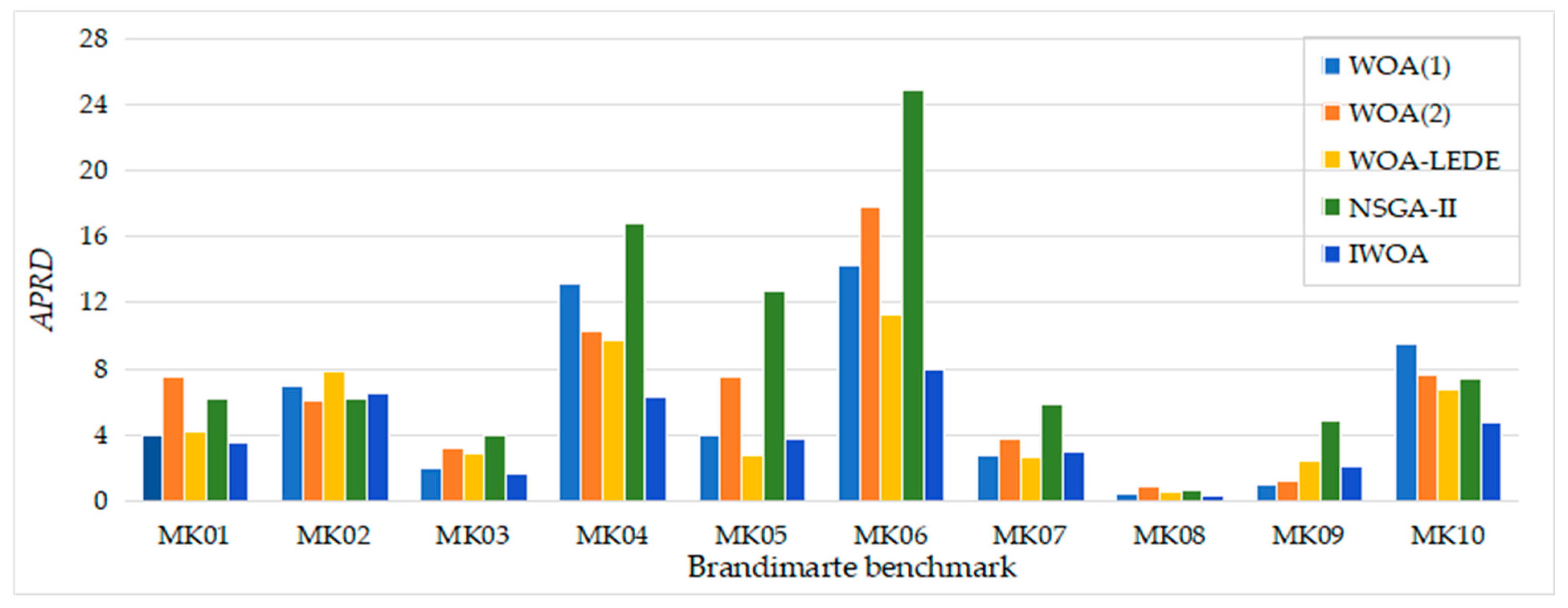
In this paper, the MATLAB 2018B programming platform was used to conduct experiments in the operating environment of Intel(R)Core(TM) I7-8550 CPU, 1.80 GHZ main frequency, and 16.0 GB memory, in order to verify the effectiveness of IWOA in solving the green FJSP using AGV transportation.

4.1. Benchmark Test

In this paper, 10 FJSP instances in the standard test set of Brandimarte [44] were selected for the simulation experiments. Different examples were independently run 20 times. Compared with Luan’s IWOA(1) [41], Jiang’s IWOA(2) [42], Liu’s WOA-LEDE [43], and the non-dominant sorting genetic algorithm (NSGA-II) commonly used for shop floor scheduling solutions, this paper carried out a comparative analysis.

Among them, the first three algorithms were applied to shop scheduling problems and showed excellent performance. These algorithms are highly similar to the algorithm proposed in this paper, and they are all improved algorithms based on the whale optimization algorithm. Therefore, compared with the above algorithms, it can fully prove whether the improvement strategy proposed by the algorithm in this paper is effective. On the other hand, the corresponding literature has compared the above three optimization whale algorithms with some excellent algorithms such as KBACO, TSPCB, HGWO, etc. [39,40,41]. Experimental results have shown that the above three improved algorithms can outperform their comparison algorithms in most optimization problems. Therefore, the performance of the proposed algorithm can be effectively verified by comparing it with the above three algorithms of the same type. In addition, NSGA-II is a classical algorithm based on genetic algorithm, which is also a popular algorithm at present. It has been applied to solve various optimization problems [45,46], so this algorithm was also used as the comparison algorithm in this paper. The parameters of these algorithms are shown in Table 2. The iteration number t_max of the above algorithm was 200, and the population size N was 100.

The comparison results of the benchmark examples are shown in

Table 3. Comparison results of the Brandimarte benchmark examples.

Instance	Oij × mk	LB	IWOA(1)		IWOA(2)		WOA-LEDE		NSGA-II		IWOA
			Best	SD	Best	SD	Best	SD	Best	SD	Best	SD
MK01	10 × 6	39	40	0.60	41	0.85	39	0.51	41	0.7	39	0.50
MK02	10 × 6	26	27	0.65	26	0.79	27	0.75	29	1.17	26	0.74
MK03	15 × 8	204	204	3.59	207	2.53	204	3.36	207	3.39	207	3.18
MK04	15 × 8	60	65	3.25	60	4.81	62	3.02	67	4.34	60	3.59
MK05	15 × 4	172	175	4.01	179	4.54	172	3.87	188	5.84	175	3.55
MK06	10 × 15	58	63	3.16	63	4.87	61	2.01	67	5.59	61	1.62
MK07	20 × 5	139	139	4.03	140	4.3	139	3.86	142	4.58	139	4.16
MK08	20 × 10	523	523	3.56	523	4.46	523	3.11	523	4.12	523	3.46
MK09	20 × 10	307	307	3.68	307	4.01	312	3.55	317	5.86	309	3.27
MK10	20 × 15	198	214	4.37	206	5.17	206	4.26	208	6.63	205	3.64

. In the table, Best represents the best result in 20 tests, SD refers to the standard deviation of the results of 20 tests, and LB is the best value found so far.

Figure 5 shows the APRD value obtained by IWOA(1), IWOA(2), WOA-LEDE, NSGA-II, and IWOA by solving 10 benchmark instances. APRD represents the average percentage deviation between 20 experimental results and LB, and the calculation formula is as follows:

$$APRD=\frac{1}{n}{\displaystyle \sum _{i=1}^n\frac{C_i-LB}{LB}}\times 100$$

(29)

where C_i is the makespan obtained by the algorithm.

It can be seen from the data in Table 3 that IWOA had the best optimization performance in MK01, MK02, MK04, MK07, and MK08, obtaining the optimal value of the optimal objective function. In MK06 and MK10, although the optimal solution was not obtained, the solution was better than the comparison algorithm. Among the three benchmark instances MK03, MK05, and MK09, the accuracy of the proposed IWOA was slightly lower than that of IWOA(1), WOA-LEDE, and WOA(2). According to the above analysis, it is not obvious that the proposed algorithm is significantly better than the other three comparison algorithms, but compared with the other three improved whale optimization algorithms, the proposed algorithm has strong competitiveness.

In terms of algorithm stability, the proposed algorithm had the best robustness performance on the five instances MK01, MK05, MK06, MK09, and MK10, and the obtained standard deviation was the smallest. The IWOA designed in this paper has certain advantages in solving accuracy and stability, the solution results were significantly better than those of NSGA-II algorithm, and it performed well in most of the 10 instances.

In Figure 5, the IWOA obtained the minimum value of APRD in seven out of 10 instances, which further proves that the proposed model has superior performance and can obtain relatively optimal and stable solutions on different scale shop scheduling problems. In summary, the optimization comparison results based on benchmark examples verified the feasibility and effectiveness of the proposed algorithm. In addition, we will further verify the superiority of the algorithm in Section 4.3, detailing the workshop example simulation.

4.2. Effectiveness of Improvement Strategy

As shown in Section 3.3, three strategies were adopted for the WOA (Strategy I: Nonlinear convergence factor; Strategy II: Nonlinear adaptive inertia weight; Strategy III: Improve the screw position update model). To analyze the contribution of different strategies to the model, the optimization effects of the IWOA (adopting three strategies), IWOA-I (adopting strategy I), IWOA-II (adopting strategy II), and IWOA-III (adopting strategy III) were compared in five instances. These five instances were the best cases solved by the IWOA in Table 3. Each algorithm was separately run 10 times. The comparison results of the above four algorithms are shown in

Table 4. Comparison of the optimization results of different strategies.

Instance	IWOA		IWOA-I		IWOA-II		IWOA-III
	APRD	Time [s]	APRD	Time [s]	APRD	Time [s]	APRD	Time [s]
MK01	3.54	7.41	8.72	6.56	4.32	7.85	3.77	8.55
MK02	6.53	13.84	7.45	8.42	6.94	15.68	7.44	17.24
MK04	6.27	21.45	12.62	17.28	7.81	28.74	8.15	24.31
MK07	3.01	25.31	5.33	29.69	4.84	29.43	3.92	32.58
MK08	2.15	45.80	14.47	51.61	6.63	51.84	4.97	55.67
Average	4.30	22.76	9.72	22.71	6.12	26.708	5.65	27.67

.

According to Equation (29), the larger the value of APRD, the more the target value of the algorithm deviates from the optimal value of the objective function, and the worse the performance of the algorithm. Computer results showed that the IWOA with the three strategies had the best performance on the five instances. The APRD of the proposed algorithm was significantly better than that of IWOA-I, IWOA-II and IWOA-III. Meanwhile, its time on MK07 and MK08 was better than that of the comparison algorithm, which showed the effectiveness of the combined application of the three strategies.

(1)

Effectiveness of nonlinear convergence factor: For comparison, the convergence speed of IWOA-I in the three small-scale instances MK01, MK02, and MK03 was greater than that of IWOA. Furthermore, it can also be calculated that the average running time difference between IWOA-I and IWOA in the five instances was −0.05 (22.71 − 22.76 = −0.05), and the average convergence speed of IWOA-I was ahead of the IWOA. The results show that the nonlinear convergence factor has a very important and positive effect on the convergence speed of the algorithm. This result from the convergence factors is a decrease nonlinearly with the increase in the number of evolutionary iterations, which ensures that whales conduct a global search with a large stride in the early stage of search, and conduct local optimization with a small stride in the later stage to improve the speed of the whole search process while ensuring the quality.

(2)

Effectiveness of nonlinear adaptive inertia weight: For the APRD value, the average difference between IWOA-II and IWOA (6.12 − 4.30 = 1.82) was significantly smaller than that between IWOA-I and IWOA (9.72 − 4.30 = 5.42), indicating that the nonlinear adaptive inertia weight has a greater impact on the optimization ability of the IWOA than the nonlinear convergence factor. In addition, for instance MK07 in Table 4, the optimization time of IWOA-II is better than that of IWOA-I, which shows that the nonlinear adaptive weight strategy can also accelerate the convergence speed of the algorithm.

(3)

Effectiveness of screw position update model: Compared with the two whale optimization algorithms based on Strategy I and Strategy II, the average APRD value of IWOA-III was closer to the whale optimization algorithm using three combined strategies, but the running time of the algorithm was inferior to IWOA-I and IWOA-II, which indicates that the screw position update model had the greatest impact on the model optimization accuracy. This result from the screw position update model can increase the diversity of the total group, which can effectively avoid the algorithm from falling into the local optimum, although the search time for the optimal solution increases.

To sum up, the three improvement strategies play different roles in the IWOA. Strategy I contributes the most to the convergence performance of the algorithm, Strategy II plays a role in both the convergence performance and the optimization accuracy of the algorithm, and Strategy III mainly improves the quality of the population by enhancing the diversity of the population. The collaboration of the three strategies strengthens the balance between the development ability of the global search and the mining ability of the local search.

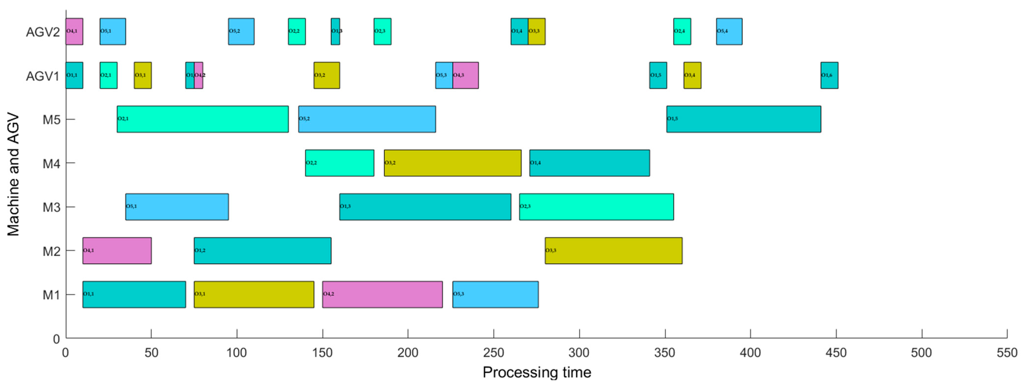
4.3. Workshop Example Simulation

This paper took the instances in

Table A1. Case 5 × 5 work-piece processing time.

	Machine (Setup Time/Processing Time/Processing Quality/Average Energy Consumption Coefficient)
Job	Oper.	M1	M2	M3	M4	M5
J1	O11	5/60/0.80/2.1	4/52/0.84/2.6	-	5/65/0.80/1.8	-
	O12	-	5/80/0.85/1.8	7/70/0.80/2.4	-	5/75/0.87/2.60
	O13	7/110/0.80/1.9	5/90/0.75/2.3	4/100/0.78/2.5	-	6/1000.85/2.5
	O14	4/77/0.80/2.5	-	6/70/0.75/1.8	5/70/0.85/1.7	4/60/0.81/2.3
	O15	5/90/0.77/2.5	7/105/0.85/2.9	-	-	5/90/0.88/3.1
J2	O21	5/82/0.77/2.5	-	4/95/0.81/2.9	7/95/0.87/3.2	5/100/0.85/2.9
	O22	-	4/50/0.75/2.8	5/55/0.80/3.5	5/40/0.78/3.5	-
	O23	-	8/70/0.76/2.0	5/90/0.82/1.8	-	5/75/0.78/2.5
J3	O31	5/70/0.85/3.3	-	5/60/0.81/2.8	-	8/70/0.82/2.8
	O32	-	5/78/0.74/2.2	-	6/80/0.79/1.8	8/83/0.82/2.5
	O33	-	5/80/0.87/2.9	4/92/0.85/2.7	5/80/0.82/2.5	-
J4	O41		5/40/0.87/1.6	-	8/48/0.88/2.5	5/45/0.82/2.1
	O42	5/70/0.80/2.6	-	7/70/0.85/2.5	5/88/0.79/2.2	-
J5	O51	-	-	8/60/0.84/1.2	8/65/0.85/2.5	5/65/0.87/2.0
	O52	-	4/80/0.78/2.8	-	4/75/0.83/2.9	6/80/0.88/3.3
	O53	6/50/0.83/3.6	8/65/0.85/3.2	6/55/0.76/2.9	5/50/0.78/3.5	-
μk		0.3	0.2	0.3	0.4	0.5
σk		0.8	0.6	0.7	1.1	0.8

and

Table A2. Case 15 × 5 work-piece processing time.

	Machine (Setup Time/Processing Time/Processing Quality/Average Energy Consumption Coefficient)
Job	Oper.	M1	M2	M3	M4	M5
J1	O11	5/110/0.88/2.3	5/105/0.87/1.6	4/100/0.84/1.8		6/95/0.79/2.5
	O12	8/95/0.84/2.7	4/80/0.82/2.3	5/85/0.81/2.3	5/65/0.80/2.7	7/85/0.75/2.2
	O13	5/80/0.75/2.1	5/85/0.82/2.4		6/70/0.85/2.5
	O14	7/60/0.88/3.1		5/55/0.82/2.5	4/60/0.75/2.3	5/50/0.81/2.7
	O15	8/85/0.82/2.5	5/95/0.77/2.3		5/100/0.80/2.5	6/90/0.84/2.9
J2	O21	7/100/0.77/2.3	3/120/0.80/2.5	4/110/0.81/2.3		4/100/0.83/2.9
	O22	5/45/0.78/1.9	4/58/0.82/1.8		6/40/0.80/2.2	7/55/0.81/2.3
	O23	7/60/0.85/2.6	4/45/0.82/2.8	5/50/0.83/2.4	5/35/0.80/3.1
J3	O31	4/70/0.83/2.5	5/80/0.85/2.3		6/75/0.80/2.0	5/60/0.83/3.0
	O32	5/25/0.75/2.2	6/30/0.84/2.8		7/20/0.82/2.4	5/20/0.80/2.2
	O33		5/50/0.85/2.5	5/60/0.83/2.5	7/55/0.85/2.1	6/40/0.78/1.8
J4	O41	5/45/0.81/2.3	6/40/0.79/2.5	7/55/0.82/2.8		5/40/0.84/2.8
	O42	7/70/0.86/2.3	5/60/0.85/1.8		4/70/0.81/2.0
J5	O51	5/60/0.80/2.2		6/60/0.84/2.4	5/75/0.77/2.0
	O52	6/85/0.81/2.3	4/90/0.80/1.9	6/70/0.77/2.3		7/80/0.84/2.8
	O53	7/50/0.80/2.1	7/65/0.83/2.3		5/60/0.80/2.3
J6	O61	8/35/0.76/2.8		6/30/0.80/3.1	4/30/0.85/3.7	4/45/0.82/3.2
	O62	7/50/0.84/2.4	3/50/0.75/2.1	6/45/0.82/2.5	5/60/0.78/2.5
	O63		5/75/0.75/2.5	6/75/0.78/2.8	7/80/0.84/3.1	5/95/0.81/2.8
J7	O71	6/55/0.77/3.1	5/65/0.82/2.6			5/70/0.85/2.8
	O72		4/30/0.82/2.3	5/25/0.78/2.3	5/40/0.85/2.6
	O73	5/55/0.84/1.9	5/60/0.80/2.3		6/50/0.84/2.7	7/38/0.75/2.6
	O74	7/100/0.82/3.5	5/110/0.84/3.8		4/90/0.79/3.5	5/105/0.78/2.6
J8	O81	4/90/0.85/1.8	5/100/0.78/2.3	3/85/0.87/2.4	6/105/0.74/2.3
	O82	6/70/0.88/2.8		4/80/0.78/2.5	4/75/0.84/2.8	7/80/0.85/2.9
	O83		5/70/0.75/1.8	6/80/0.83/2.2	4/80/0.75/1.6	5/90/0.85/2.0
J9	O91		5/100/0.79/2.1	5/90/0.82/2.5	6/100/0.85/2.7
	O92	7/75/0.79/2.4		6/60/0.82/2.4		7/70/0.81/2.7
J10	O10,1		7/80/0.84/2.7	5/70/0.77/1.8	5/70/0.80/2.3	5/85/0.78/1.9
	O10,2	6/55/0.77/3.2	4/40/0.75/2.8	5/50/0.86/2.4
	O10,3	7/110/0.76/2.3	5/95/0.88/2.7	4/90/0.78/2.5		6/100/0.85/2.5
J11	O11,1	5/30/0.76/2.7		4/30/0.83/2.7	5/35/0.85/2.3	5/45/0.75/2.2
	O11,2	4/85/0.85/2.6	7/80/0.78/2.2	5/90/0.84/2.5	5/80/0.84/2.7
	O11,3		4/50/0.78/1.6	5/60/0.83/2.5	7/55/0.81/2.7	7/60/0.80/2.1
J12	O12,1	7/75/0.78/1.9	6/65/0.81/2.3		5/70/0.85/2.3
	O12,2	4/60/0.81/2.3			5/60/0.78/2.3	7/50/0.81/2.9
	O12,3		5/110/0.82/2.3	5/100/0.84/2.6		7/110/0.78/2.0
	O12,4	8/80/0.80/1.9	6/80/0.83/2.5	4/60/0.80/2.2	4/70/0.81/2.7
J13	O13,1	5/70/0.78/2.1		5/65/0.81/3.8	6/80/0.85/2.6
	O13,2	3/20/0.80/2.0	4/30/0.76/2.9	4/30/0.78/2.0	7/20/0.80/2.5
	O13,3		6/50/0.81/2.5	5/50/0.78/2.1	7/40/0.78/2.9	5/60/0.83/2.5
J14	O14,1	5/85/0.80/2.8	5/90/0.83/2.5			6/100/0.86/2.4
	O14,2		5/80/0.84/2.8		6/70/0.80/2.2	7/65/0.76/2.1
	O14,3	5/40/0.83/2.7		6/50/0.82/2.5	5/35/0.78/2.2
	O14,4	7/60/0.80/2.1	7/40/0.80/2.4	4/50/0.83/2.6		5/55/0.78/2.4
J15	O15,1	5/60/0.81/3.1	7/70/0.80/2.6	5/50/0.85/3.3
	O15,2	7/25/0.75/1.8		6/30/0.82/2.3	6/40/0.82/2.0	4/35/0.83/2.5
	O15,3	3/65/0.88/2.2	7/40/0.81/2.8		5/50/0.83/2.8	5/55/0.85/3.3
μk		0.3	0.2	0.3	0.4	0.5
σk		0.8	0.6	0.7	1.1	0.8

(refer to Appendix A) as the research object, and solved the green FJSP problem with the makespan, workshop energy consumption, and processing quality as the optimization goals. The transportation energy consumption of the AGV was generated randomly in [2.0, 2.5] [47]. Furthermore, from a cost-saving perspective, we aimed to use the minimum number of AGVs under the premise of achieving multi-objective optimization. Therefore, in the given instances, the upper limit for the number of AGVs was set to 3 for Instance 5 × 5 and 6 for Instance 15 × 5. The transportation times between different machines are shown in

Table 5. The transportation times of AGVs between machines (unit: seconds).

Machine Number	M0	M1	M2	M3	M4	M5	M6
M0	0	10	15	20	20	10	15
M1	10	0	5	10	20	15	20
M2	15	5	0	5	15	15	15
M3	20	10	5	0	10	20	10
M4	20	20	15	10	0	10	10
M5	10	15	15	20	10	0	20
M6	15	20	15	10	10	20	0

Note: M₀ is the unprocessed job storage area, M₁–M₅ are the machines, and M₆ is the finished job storage area.

.

(1) Solution of the multi-objective model

Figure 6 shows the feasible solutions for the Instance 5 × 5, satisfaction μ ≥ 0.6. The number of feasible solutions obtained by IWOA was 10, and the feasible solutions of WOA(1), WOA(2), WOA-LEDE, and NSGA-II were 7, 8, 12, and 7.

Table 6. Maximum satisfaction value of the optimization results with different algorithms.

	μ	μ1	μ2	μ3	Z1	Z2	Z3
WOA(1)	0.726	0.70	0.89	0.59	449	3784	0.827
WOA(2)	0.720	0.76	0.55	0.85	445	4004	0.836
WOA-LEDE	0.743	0.70	0.85	0.68	449	3808	0.830
NSGA-II	0.715	0.55	0.83	0.76	459	3823	0.833
IWOA	0.747	0.67	0.75	0.82	451	3918	0.834

shows the objective function value when the overall satisfaction of the above algorithm is optimal. Figure 7 is the comparison result of the membership degree μ of each objective function.

According to the calculation results, the optimal satisfaction value μ = 0.749 was obtained by IWOA, the makespan of workshop Z1 = 451, the energy consumption of workshop Z2 = 3918, and the processing quality Z3 = 0.834.

Compared to the optimal makespan goal Z1*, the actual makespan Z1 increased by 22 units, resulting in a −33% degree of optimization. However, when measured against other optimal completion times Z2* and Z3*, Z1 showed a reduction of 45 and 32 units, with optimization degrees of 48% and 67%, respectively.

In relation to the optimal energy consumption goal Z2*, the observed energy consumption Z2 rose by 167 units, marking a −25% degree of optimization. Conversely, it witnessed a decrease of 440 and 237 units compared to the energy consumptions of Z1* and Z3*.

Compared with the optimal processing quality Z3*, the processing quality of Z3 was reduced by 0.0063 (optimization degree was −18%). Nevertheless, Z3 was increased by 0.019 (optimization degree is 58%) and 0.027 (optimization degree is 82%) compared with the processing quality of Z1* and Z2*.

The analysis clearly underscores the necessity and efficacy of a multi-objective model to enhance production quality while concurrently reducing energy consumption in the workshop setting. It is crucial to recognize that in the realm of multi-objective optimization, a single “optimal” solution encompassing all objectives is generally unattainable. The improvement of one objective often comes at the expense of another, highlighting the intrinsic trade-offs involved. Utilizing a satisfaction function, constructed based on fuzzy membership degree theory, provides decision-makers with a range of viable solutions. This flexibility allows for a balanced evaluation of the economic, environmental, and production-related benefits, enabling the selection of an optimal strategy tailored to specific priorities. Simultaneously, the model accounts for completion time, energy efficiency, and processing quality. In doing so, it ensures that production deadlines and quality standards are met while also striving to fulfill green objectives such as energy conservation and emissions reduction.

(2) Comparison of the algorithm results

The algorithm proposed in this paper and the above-mentioned four comparison algorithms were independently run 20 times in two instances to avoid the chance of solving the algorithm. Figure 8 shows the convergence of the optimization process, and Figure 9 shows the box plot results of each algorithm run 20 times.

The above results show that the improved algorithm proposed in this paper had the best effect on the two instances, and its advantages are embodied in the following aspects:

(1)

Model convergence: From the convergence curve, the proposed IWOA algorithm had good global search performance and local information mining ability. The blue curve shows the iteration process of the IWOA. In the early stage of iteration, the curve jump distance is large, which indicates that the algorithm has better global detection ability. At the later stage of iteration, it still shows good search ability and frequent small distance down hops until finally stable, without falling into the local optimum. Formally, the convergence speed of the IWOA was better than IWOA(2) and WOA-LEDE on 5 × 5 instances. Although IWOA(1) and NSG-II converged before IWOA, their optimization effect was not good. In addition, in 5 × 15 instances, the convergence speed of IWOA was significantly better than that of the other four comparison algorithms. Therefore, it can be concluded that compared with small-scale scheduling problems, the proposed algorithm has stronger performance in large-scale numerical examples.

(2)

Model solution quality: According to the convergence curve, the loss function of the IWOA was 0.250 and 0.245, respectively, in two instances of different sizes, which is better than the loss of the comparison algorithm, and the multi-objective solution with the maximum satisfaction degree was obtained. In addition, it can be seen from Figure 9 that the mean value of loss function of IWOA in the 5 × 5 and 15 × 5 instances was 0.265 and 0.258, respectively, and its upper and lower limits were also much better than its comparison algorithm.

(3)

Stability of the model: Figure 9 shows that the loss function fluctuations of IWOA in the two instances were [0.251, 0.275] and [0.245, 0.273] respectively, which were significantly smaller than the loss fluctuation interval of the comparison algorithm. The algorithm shows good stability, and the stability performance on large-scale instances is superior.

(3) Statistical analysis

We performed statistical analysis on the experimental results. The Wilcoxon’s test was used to verify whether the differences between models with different strategies were significant. We took IWOA as the control algorithm and tested whether the difference between the proposed algorithm and the comparison algorithm was significant with 95% confidence. We defined the null hypothesis (H0) and the alternative hypothesis (H1):

H0: 

There is no significant difference in performance between the IWOA and comparison algorithms.

H1: 

There is a significant difference in performance between the IWOA and comparison algorithms.

The statistical results are shown in

Table 7. Statistical analysis of the Wilcoxon’s rank-sum test.

IWOA VS.	Instance	Statistic	p-Value	p < a (a = 0.05)
WOA(1)	5 × 5	0.0	3.815 × 10−6	yes
	15 × 5	32.0	9.452 × 10−3	yes
WOA(2)	5 × 5	0.0	3.815 × 10−6	yes
	15 × 5	19.0	1.171 × 10−3	yes
WOA-LEDE	5 × 5	37.0	1.809 × 10−2	no
	15 × 5	8.0	9.537 × 10−5	yes
NSGA-II	5 × 5	0.0	3.815 × 10−6	yes
	15 × 5	0.0	3.815 × 10−6	yes

, where “yes” indicates significant differences between the control algorithm and the comparison algorithm. “No” indicates that there is no significant difference between the control algorithm and the comparison algorithm. According to the p-value obtained, it can be concluded that there was a statistically significant difference between the performance of the IWOA and the four comparison algorithms, except that there was no significant difference between the IWOA and WOA LEDE on the 5 × 5 instance. This result is in line with the experimental results above, where compared with the comparison algorithm, IWOA had a more excellent optimization effect in large scale instances.

(4) Scheduling scheme

For the convergence curve above, Gantt charts of the green flexible shop scheduling scheme with maximum satisfaction is shown in Figure 10 and Figure 11. Each square in the figure represents an operation, the number in the square represents the operation number, and the square of the same color represents the same job. From the figure, the processing sequence, machine selection, and AGV transportation of each operation can be known.

5. Conclusions

With the process of automation in the manufacturing industry, the study of flexible workshops containing AGVs is more in line with the actual situation of modern workshops, and the scheduling results are more practical. In this paper, the green flexible job shop scheduling problem of machine and AGV integration was studied, a multi-objective mathematical model was established with the optimization goals of minimizing the makespan, minimizing the energy consumption of the workshop, and maximizing the production quality, and an improved whale optimization algorithm was proposed to solve it. The improvements made in the proposed whale optimization algorithm include designing encoding and decoding schemes, introducing nonlinear convergence factors and adaptive inertia weights, and improving the screw position update model to improve the optimization ability of the algorithm. In addition, the loss function of the IWOA was constructed based on fuzzy membership degree theory to obtain the optimal compromise solution of the multi-objective model. Finally, the performance of the proposed multi-objective model and algorithm was evaluated through Brandimarte benchmark instances and numerical instances, and the main conclusions are as follows:

First, based on the results of experiments using benchmark instances, the IWOA achieved the optimal completion times for the MK01, MK02, MK04, MK07, and MK08 benchmark instances, which were 39, 26, 60, 139, and 523, respectively. The standard deviations in the MK01, MK05, MK06, MK09, and MK10 benchmark instances were the smallest at 0.50, 3.44, 1.62, 3.27, and 3.63, respectively. These results demonstrate the effectiveness of the IWOA.

Furthermore, in the given two workshop instances, 5 × 5 and 15 × 5, the IWOA was able to find the optimal satisfaction values of approximately 0.747 and 0.754 in around 100 iterations. Compared to the IWOA(1), IWOA(2), WOA-LEDE, and NSGA-II algorithms, IWOA exhibited better optimization accuracy and robustness and was more competitive in large-scale cases.

Finally, by comparing the results of the single-objective optimal solutions and the multi-objective optimization solutions with maximum satisfaction, it is evident that the multi-objective model constructed in this paper is necessary and effective in improving the workshop processing quality and reducing energy consumption. This is conducive to the green development of the manufacturing industry and offers significant advantages over single-objective optimization models.

Moving forward, our research aims to explore further advancements in multi-objective optimization algorithms, potentially incorporating machine learning techniques for even more robust scheduling solutions.

References

1. Yao, X.; Lin, Y. Emerging manufacturing paradigm shifts for the incoming industrial revolution. Int. J. Adv. Manuf. Technol. 2016, 85, 1665–1676. [Google Scholar] [CrossRef]
2. Jamili, A. Robust job shop scheduling problem: Mathematical models, exact and heuristic algorithms. Expert Syst. Appl. 2016, 55, 341–350. [Google Scholar] [CrossRef]
3. Zhao, F.; Zhang, L.; Cao, J.; Tang, J. A cooperative water wave optimization algorithm with reinforcement learning for the distributed assembly no-idle flowshop scheduling problem. Comput. Ind. Eng. 2021, 153, 107082. [Google Scholar] [CrossRef]
4. Huo, L.; Wang, J.Y. Flexible job shop scheduling based on digital twin and improved bacterial foraging. Int. J. Simul. Model. 2022, 21, 525–536. [Google Scholar] [CrossRef]
5. Barak, S.; Moghdani, R.; Maghsoudlou, H. Energy-efficient multi-objective flexible manufacturing scheduling. J. Clean. Prod. 2021, 283, 124610. [Google Scholar] [CrossRef]
6. Xing, Z.; Liu, H.T.; Wang, T.S.; Chew, E.P.; Lee, L.H.; Tan, K.C. Integrated automated guided vehicle dispatching and equipment scheduling with speed optimization. Transp. Res. E Logist. Transp. Rev. 2022, 169, 102993. [Google Scholar] [CrossRef]
7. Abderrabi, F.; Godichaud, M.; Yalaoui, A.; Yalaoui, F.; Amodeo, L.; Qerimi, A.; Thivet, E. Flexible job shop scheduling problem with sequence dependent setup time and job splitting: Hospital catering case study. Appl. Sci. 2021, 11, 1504. [Google Scholar] [CrossRef]
8. Wu, X.; Sun, Y. A green scheduling algorithm for flexible job shop with energy-saving measures. J. Clean. Prod. 2018, 172, 3249–3264. [Google Scholar] [CrossRef]
9. Uzsoy, R. Scheduling a single batch processing machine with non-identical job sizes. Int. J. Prod. Res. 1994, 32, 1615–1635. [Google Scholar] [CrossRef]
10. Shi, X.Q.; Long, W.; Li, Y.Y.; Wei, Y.L.; Deng, D.S. Different performances of different intelligent algorithms for solving FJSP: A perspective of structure. Comput. Intell. Neurosci. 2018, 4617816. [Google Scholar] [CrossRef]
11. Zhou, S.; Xing, L.; Zheng, X.; Du, N.; Wang, L.; Zhang, Q. A self-adaptive differential evolution algorithm for scheduling a single batch-processing machine with arbitrary job sizes and release times. IEEE Trans. Cybern. 2019, 51, 1430–1442. [Google Scholar] [CrossRef] [PubMed]
12. Gajsek, B.; Dukic, G.; Kovacic, M.; Brezocnik, M. A multi-objective genetic algorithms approach for modelling of order picking. Int. J. Simul. Model. 2021, 20, 719–729. [Google Scholar] [CrossRef]
13. Zhao, F.; Di, S.; Cao, J.; Tang, J. A novel cooperative multi-stage hyper-heuristic for combination optimization problems. Complex Syst. Model. Simul. 2021, 1, 91–108. [Google Scholar] [CrossRef]
14. Brandão, J. Iterated local search algorithm with ejection chains for the open vehicle routing problem with time windows. Comput. Ind. Eng. 2018, 120, 146–159. [Google Scholar] [CrossRef]
15. Zheng, Y.; Xiao, Y.; Seo, Y. A tabu search algorithm for simultaneous machine/AGV scheduling problem. Int. J. Prod. Res. 2014, 52, 5748–5763. [Google Scholar] [CrossRef]
16. Umar, U.A.; Ariffin, M.K.A.; Ismail, N.; Tang, S.H. Hybrid multiobjective genetic algorithms for integrated dynamic scheduling and routing of jobs and automated-guided vehicle (AGV) in flexible manufacturing systems (FMS) environment. Int. J. Adv. Manuf. Technol. 2015, 81, 2123–2141. [Google Scholar] [CrossRef]
17. Saidi-Mehrabad, M.; Dehnavi-Arani, S.; Evazabadian, F.; Mahmoodian, V. An Ant Colony Algorithm (ACA) for solving the new integrated model of job shop scheduling and conflict-free routing of AGVs. Comput. Ind. Eng. 2015, 86, 2–13. [Google Scholar] [CrossRef]
18. Sanches, D.S.; Silva Rocha, J.D.; Castoldi, M.F.; Morandin, O.; Kato, E.R.R. An adaptive genetic algorithm for production scheduling on manufacturing systems with simultaneous use of machines and agvs. J. Control Autom. Electr. Syst. 2015, 26, 225–234. [Google Scholar] [CrossRef]
19. Nageswararao, M.; Narayanarao, K.; Rangajanardhana, G.S. Scheduling of machines and automated guided vehicles in FMS using gravitational search algorithm. Appl. Mech. Mater. 2017, 867, 307–313. [Google Scholar] [CrossRef]
20. Fazlollahtabar, H.; Hassanli, S. Hybrid cost and time path planning for multiple autonomous guided vehicles. Appl. Intell. 2018, 48, 482–498. [Google Scholar] [CrossRef]
21. Li, G.; Zeng, B.; Liao, W.; Li, X.; Gao, L. A new AGV scheduling algorithm based on harmony search for material transfer in a real-world manufacturing system. Adv. Mech. Eng. 2018, 10, 1687814018765560. [Google Scholar] [CrossRef]
22. Lyu, X.; Song, Y.; He, C.; Lei, Q.; Guo, W. Approach to integrated scheduling problems considering optimal number of automated guided vehicles and conflict-free routing in flexible manufacturing systems. IEEE Access 2019, 7, 74909–74924. [Google Scholar] [CrossRef]
23. Zhu, Z.; He, Y. An improved genetic algorithm for production scheduling on FMS with simultaneous use of machines and AGVs. In Proceedings of the 2019 11th International Conference on Intelligent Human-Machine Systems and Cybernetics (IHMSC), Hangzhou, China, 24–25 August 2019; Volume 1, pp. 245–249. [Google Scholar]
24. Lei, C.; Zhao, N.; Ye, S.; Wu, X. Memetic algorithm for solving flexible flow-shop scheduling problems with dynamic transport waiting times. Comput. Ind. Eng. 2020, 139, 105984. [Google Scholar] [CrossRef]
25. Meng, L.; Zhang, C.; Shao, X.; Ren, Y.; Ren, C. Mathematical modelling and optimisation of energy-conscious hybrid flow shop scheduling problem with unrelated parallel machines. Int. J. Prod. Res. 2019, 57, 1119–1145. [Google Scholar] [CrossRef]
26. Meng, L.; Zhang, C.; Shao, X.; Ren, Y. MILP models for energy-aware flexible job shop scheduling problem. J. Clean. Prod. 2019, 210, 710–723. [Google Scholar] [CrossRef]
27. Zhou, M.X.; Li, X. Low-carbon production control and resource allocation optimization. Int. J. Simul. Model. 2022, 21, 352–363. [Google Scholar] [CrossRef]
28. Liu, C.; Yao, Y.; Zhu, H. Hybrid salp swarm algorithm for solving the green scheduling problem in a double-flexible job shop. Appl. Sci. 2021, 12, 205. [Google Scholar] [CrossRef]
29. Liu, Q.H.; Wang, C.Y.; Li, X.Y.; Gao, L. A multi-population co-evolutionary algorithm for green integrated process planning and scheduling considering logistics system. Eng. Appl. Artif. Intell. 2023, 126, 107030. [Google Scholar] [CrossRef]
30. Jiang, T.; Zhang, C.; Sun, Q.M. Green job shop scheduling problem with discrete whale optimization algorithm. IEEE Access 2019, 7, 43153–43166. [Google Scholar] [CrossRef]
31. Yao, F.; Alkan, B.; Ahmad, B.; Harrison, R. Improving just-in-time delivery performance of IoT-enabled flexible manufacturing systems with AGV based material transportation. Sensors 2020, 20, 6333. [Google Scholar] [CrossRef]
32. Jiang, T.; Zhu, H.; Deng, G. Improved African buffalo optimization algorithm for the green flexible job shop scheduling problem considering energy consumption. J. Intell. Fuzzy Syst. 2020, 38, 4573–4589. [Google Scholar] [CrossRef]
33. Peng, Z.; Zhang, H.; Tang, H.; Feng, Y.; Yin, W. Research on flexible job-shop scheduling problem in green sustainable manufacturing based on learning effect. J. Intell. Manuf. 2021, 33, 1725–1746. [Google Scholar] [CrossRef]
34. Afsar, S.; Palacios, J.J.; Puente, J.; Vela, C.R.; González-Rodríguez, I. Multi-objective enhanced memetic algorithm for green job shop scheduling with uncertain times. Swarm Evol. Comput. 2022, 68, 101016. [Google Scholar] [CrossRef]
35. Chen, J.X.; Wu, Y.X.; Huang, S.; Wang, P. Multi-objective optimization for AGV energy efficient scheduling problem with customer satisfaction. AIMS Math. 2023, 8, 20097–20124. [Google Scholar] [CrossRef]
36. Mirjalili, S.; Lewis, A. The whale optimization algorithm. Adv. Eng. Softw. 2016, 95, 51–67. [Google Scholar] [CrossRef]
37. Li, A.D.; He, Z. Multiobjective feature selection for key quality characteristic identification in production processes using a nondominated-sorting-based whale optimization algorithm. Comput. Ind. Eng. 2020, 149, 106852. [Google Scholar] [CrossRef]
38. Zeng, N.; Song, D.; Li, H.; You, Y.; Liu, Y.; Alsaadi, F.E. A competitive mechanism integrated multi-objective whale optimization algorithm with differential evolution. Neurocomputing 2021, 432, 170–182. [Google Scholar] [CrossRef]
39. Abd Elaziz, M.; Lu, S.; He, S. A multi-leader whale optimization algorithm for global optimization and image segmentation. Expert Syst. Appl. 2021, 175, 114841. [Google Scholar] [CrossRef]
40. Yang, S.; Chen, D.; Li, S.; Wang, W. Carbon price forecasting based on modified ensemble empirical mode decomposition and long short-term memory optimized by improved whale optimization algorithm. Sci. Total Environ. 2020, 716, 137117. [Google Scholar] [CrossRef]
41. Luan, F.; Cai, Z.; Wu, S.; Jiang, T.; Li, F.; Yang, J. Improved whale algorithm for solving the flexible job shop scheduling problem. Mathematics 2019, 7, 384. [Google Scholar] [CrossRef]
42. Jiang, T.; Zhang, C.; Zhu, H.; Gu, J.; Deng, G. Energy-efficient scheduling for a job shop using an improved whale optimization algorithm. Mathematics 2018, 6, 220. [Google Scholar] [CrossRef]
43. Liu, M.; Yao, X.; Li, Y. Hybrid whale optimization algorithm enhanced with Lévy flight and differential evolution for job shop scheduling problems. Appl. Soft Comput. 2020, 87, 105954. [Google Scholar] [CrossRef]
44. Brandimarte, P. Routing and scheduling in a flexible job shop by tabu search. Ann. Oper. Res. 1993, 41, 157–183. [Google Scholar] [CrossRef]
45. Rahimi, I.; Gandomi, A.H.; Deb, K.; Chen, F.; Nikoo, M.R. Scheduling by NSGA-II: Review and bibliometric analysis. Processes 2022, 10, 98. [Google Scholar] [CrossRef]
46. Zhu, J.; Wang, X.; Huang, H.; Cheng, S.; Wu, M. A NSGA-II algorithm for task scheduling in UAV-enabled MEC system. IEEE Trans. Intell. Transp. Syst. 2021, 23, 9414–9429. [Google Scholar] [CrossRef]
47. Li, H.; Zhu, H.; Jiang, T. Modified migrating birds optimization for energy-aware flexible job shop scheduling problem. Algorithms 2020, 13, 44. [Google Scholar] [CrossRef]
Figure 1. Flowchart of the whale optimization algorithm.
Applsci 13 11896 g001
Figure 2. Whale individual coding vector matrix. The first line of numbers in OS represents the workpiece number; the second line of numbers in MS represents the machine number; and the third line of numbers in VS represents the AGV number.
Applsci 13 11896 g002
Figure 3. Ladder fuzzy membership.
Applsci 13 11896 g003
Figure 4. The multi-objective membership model construction process.
Applsci 13 11896 g004
Figure 5. Histogram of the APRD values obtained by five algorithms.
Applsci 13 11896 g005
Figure 6. Distribution of feasible solutions for Instance 5 × 5.
Applsci 13 11896 g006
Figure 7. Comparison of membership values.
Applsci 13 11896 g007
Figure 8. Convergence curves of different algorithms.
Applsci 13 11896 g008
Figure 9. Boxplot of 20-times solution results.
Applsci 13 11896 g009
Figure 10. Gantt chart of Instance 5 × 5 scheduling.
Applsci 13 11896 g010
Figure 11. Gantt chart of Instance 15 × 5 scheduling.
Applsci 13 11896 g011