Abstract
The authors of this paper focused their attention on developing numerical models of mechanical wave propagation along human tissue as a result of the application of the measuring head of the FibroScan® elastograph. The FibroScan® diagnostic device is used for diagnostic testing of liver fibrosis and steatosis. This examination is carried out using an in vivo method by directly applying the surface of the ultrasonic measuring probe to the patient’s skin at the site of the liver. The authors’ idea is to use this apparatus for non-invasive testing on the liver used for transplantation. In order to do this, the measuring head cap should be modified so that its application to the liver does not result in damage as a result of mechanical wave excitation. The purpose of the manuscript was to build numerical models of the liver and the tissues surrounding the liver. Then, the corresponding numerical simulations were carried out, the results of which corresponded to the mechanical–acoustic properties of the physical models of the tissues. The obtained results were validated on a set of commercial calibrated phantoms. High agreement of the numerical models was obtained.
1. Introduction
Diagnostic tools used in assessing the condition of human organs are now widely used. Such a device is the FibroScan® elastograph, the measuring head of which generates a mechanical wave in contact with the skin and at the same time sends out ultrasound to measure the speed of wave propagation and its attenuation, making it possible to determine the degree of liver fibrosis and steatosis. Two ultrasound heads are available: the M head for universal use and the XL head dedicated to people with obesity. The advantages of the test are repeatability, non-invasiveness, speed, and high diagnostic value [1].
The tests used in transplantation to assess organ function and suitability for transplantation have their limitations, and none of them meet the condition of non-invasiveness in assessing the degree of fibrosis and steatosis of the organ, which are currently assessed only by biopsy examination. Despite its drawbacks, conventional liver biopsy, where formal histological analysis takes place, remains the best available method for quantitative assessment of liver steatosis. The use of the FibroScan® device can be helpful in the non-invasive evaluation of liver suitability for transplantation, complementing diagnostic methods, in view of the short time (approximately 12 h) that liver harvested for transplantation can be stored and evaluated [2,3].
There is a narrow range of available literature describing the use of transient elastography including the FibroScan® device to assess liver fibrosis by measuring liver stiffness. In his study, Sánchez and his research team focused on assessing fibrosis in liver transplantation and investigating the relationship between obesity and normal test results [2]. The experimental group consisted of 29 patients who underwent liver transplantation in 2008, and he noted that the use of the FibroScan® device allows the volume of the test sample to be almost 100 times larger than that of a classic biopsy [4]. However, this technique does not work well in obese patients whose body mass index (BMI) is above 28 kg/m2 and in cases of ascites. The probe of the device used was applied through the intercostal spaces to the right lobe of the liver [5]. A success rate of at least 60% in performing the test was achieved. The final result was that almost one in five patients could not be examined properly because they were overweight or had ascites. A BMI value above 30 kg/m2 resulted in an incremental test abnormality of up to 50%. In view of these conclusions, attempts are underway to develop a specialized FibroScan® probe for obese patients to minimize the error rate.
A research group from India led by Rajamani conducted a 2022 review of techniques and trends in the diagnosis of liver steatosis in donors [3]. They paid particular attention to the study of macrovesicular steatosis in the livers of deceased and living donors. They emphasized that elevated levels of macroalveolar steatosis are directly associated with adverse outcomes in liver transplantation. One of the non-invasive diagnostic methods included in the analysis was ultrasound using the FibroScan® device, where the difference in value between a fat-laden hepatocyte and a normal hepatocyte was examined. The use of the backscattered amplitude of the ultrasound wave was adopted as the device’s operating algorithm to analyze the intensity of this signal. Setting the attenuation parameter in the range of 100–400 dB/m results in increased penetration of fat in the liver [6,7]. Through studies conducted on deceased donor organs, it has been found that there is a directly proportional relationship between the results of the FibroScan® device and the success of liver transplantation. It has been found that the device, in addition to being non-invasive, also allows a much larger area of the organ to be covered during the examination than a conventional liver biopsy. This makes it possible to reduce the error due to the size of the examined sample. The main designated disadvantages of the aforementioned test are calibration error, poor penetration in overweight individuals, and a lack of continuous follow-up.
The essence of the problem of applying the probe to an open liver may be the mechanical trauma resulting from the application of the probe and from the generation of a transverse wave of 50 Hz frequency and amplitude negatively affecting liver tissue. Based on the literature review, it is concluded that there is a significant gap with respect to the use of variable FibroScan® caps to improve test results. In view of the above, there is a need to develop numerical models, on the basis of which it is possible to quickly make a preliminary assessment of the propagation of mechanical waves along the liver tissue, among other parameters. The construction of such models is associated with the development of geometric models of the liver organ system and material mimicking the layer of skin and tissue surrounding the liver, followed by the adoption of appropriate initial-boundary conditions in the simulation. This approach will allow the authors of this paper to develop a suitable methodology for further work on the development of caps for the measuring heads of the FibroScan® elastograph in adaptation to the transplantation diagnosis of the liver.
In view of the research problems presented above, the purpose of this paper is to present preliminary analyses of mechanical wave propagation in the analyzed system for non-invasive assessment of liver condition. The authors aim to obtain satisfactory results with respect to the modification of the measuring head cap, so that following its application to the liver there is no damage due to the excitation of the mechanical wave.
2. Description of the Problem
Based on an analysis of the literature on the subject and our own research [8], it was found that it is very important to determine the parameters necessary for the construction of numerical models, including rheological models, and to choose such a model that will provide an optimal solution and approximation of the physical model. One of the important elements is the determination of the value of the propagation velocity of the ultrasonic longitudinal wave, c, ranging from about 1410 m/s in fat to about 1630 m/s in muscle. Other key parameters are Young’s modulus and Poisson’s ratio for the elastic range of the test medium. On the other hand, the measuring head generates two types of waves: a low-frequency (50 Hz) transverse wave of high amplitude and a high-frequency (ultrasound 2–3 MHz) longitudinal wave. Based on the analyses, it is concluded that the speed and length of the generated transverse wave with a frequency of 50 Hz [8] do not significantly affect the transmission of the mechanical transverse wave to the liver parenchyma. The reason is that the thicknesses of all the layers on the path from the surface of the measuring head to the liver parenchyma (skin, adipose tissue, muscle tissue, pleural cavity with serous fluid, diaphragm, peritoneal fluid between the peritoneal membranes, liver capsule membrane) are smaller than the length of the applied wave.
The liver is the largest gland in the human body. It weighs an average of 1.5 kg and contains more than 450 mL of blood. Averaged dimensions for the population are 280 × 160 × 80 mm. Figure 1 shows an image of the liver viewed from the diaphragmatic and visceral surfaces [9].
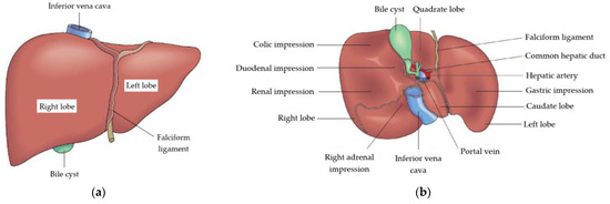
Figure 1.
Liver: (a) anterior view, diaphragmatic surface, (b) posterior view, visceral surface [9].
The FibroScan® device is mainly used for transcutaneous examinations, in which wave propagation is carried out sequentially through soft tissue and the liver. The examination takes place on the surface between the ribs, and their close presence can affect wave propagation. A typical in vivo study is shown in Figure 2a. The authors of the study paid special attention to the use of the measuring head of the FibroScan® device on the so-called living liver, rather than its percutaneous use, as in the classical application. In view of the above, the head should be reconstructed by developing an additional overlay to replicate the surface between the skin and the liver. In the process of creation, special attention should be paid to matching the appropriate properties to replace the soft structures, i.e., the fraction from the skin to the liver (Figure 2b). This operation will allow the soft structures present to be taken into account during the test, so that the waveform parameters for the test on the living liver are the same as for the transcutaneous test.
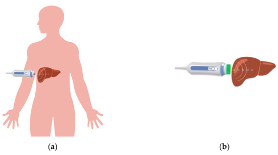
Figure 2.
Schematic of liver examination using the ultrasound head of the FibroScan® instrument: (a) in vivo, (b) the idea of application on a living liver.
Modelling the soft tissue system and liver from the point of view of numerical analysis poses significant challenges. Few studies have been devoted to these issues in the literature [10]. Numerical simulation of ultrasound waves in the range of 2.0–3.0 MHz requires an appropriate methodological approach. The first stage of the study consisted of modelling the system (the liver, skeletal system, muscular system, and skin) and an indenter imitating a scanning head corresponding to the system of human anatomy. The thicknesses of the various layers were developed based on human cross sections taken in vivo at the level of the vertebral bodies of the tenth thoracic and first lumbar vertebrae [11]. Based on the literature review, two mathematical models were selected in describing the rheology of liver tissue structure, namely, the so-called parenchymal structure models of Yeoha and Ogden [12].
3. Assumptions for Numerical Modelling
It is very common for studies to simplify by using a linear elastic model to describe the properties of soft tissues. Together with the assumption of incompressibility and isotropy of these tissues, this greatly simplifies calculations. The linear elastic model also makes it possible to describe material subjected to different types of loading. This idea is too general and already has an error in its assumption due to the nature of the linearity of the rheological response of the material [13,14].
Another approach involves approaching tissue structure by describing it with hyperelastic models [10]. Both of these classes of models can provide useful predictions of the mechanical behaviour of different elastomers/soft tissues. Table 1 summarises the strain energy density functions of commonly used hyperelastic models.

Table 1.
Density energy functions of model deformations.
Due to the complexity of the model itself and the number of component inputs in the further stage of the study, it was decided to consider two hyperelastic rheological models, the Ogden model and the Yeoh model. The aforementioned models do not require complex calculations and are successfully applied in the literature to fit the mechanical response of the liver. After preliminary simulations of the excitation of mechanical wave propagation in the liver by simulating the loading of the surrogate model with spherical, flat, and rounded tip indenters, the tuning of the ultrasound wave in biological media proceeded. Tuning was carried out with forcing by an ultrasonic signal with a frequency of f = 3.0 MHz.
Yeoh’s hyperelastic material model is a phenomenological model of deformation of nearly incompressible, nonlinear elastic materials such as elastomers. The model is based on Ronald Rivlin’s observation that the elastic properties of rubber can be described by a strain energy density function, which is a power series in strain invariants. Since the polynomial form of the strain energy density function is used, but not all three invariants of the left Cauchy–Green strain tensor, Yeoh’s model is also called the reduced polynomial model.
Yeoh’s mathematical model is shown below:
where Ci0, Di are the material constants; I1 represents invariants of the Cauchy–Green deformation tensor; is the volume ratio after and before deformation; λi represents principal stretches; is the shear modulus; and is the bulk modulus.
The values of the material constants used for the Yeoh model were obtained through in-house experiments. The results are shown below in Table 2.
Table 2.
Material constants of the Yeoh model.
The Ogden material model is a hyperelastic material model used to describe the nonlinear stress–strain behavior of complex materials such as rubbers, polymers, and biological tissue. The model developed by Raymond Ogden, like other hyperelastic material models, assumes that their behavior can be described by a strain energy density function from which the stress–strain relationship can be derived. In Ogden’s material model, the strain energy density is expressed in terms of principal stretches λj, j = 1, 2, 3.
Here, and are the material constants and λi represents principal stretches.
The material constants, and , used in the Ogden model are usually determined experimentally. Knowing as little as one of them makes it possible to obtain an optimal approximation of the data under study. The values of the constants used were obtained by experimental self-study and are shown in Table 3.
Table 3.
Material constants of the Ogden model.
Considering an incompressible material under uniaxial stretching, with the stretch factor given as λ = l/l0, where l is the stretched length and l0 is the original unstretched length, the following relation is obtained:
where , , and are the material constants, λi represents principal stretches, is the volume ratio after and before deformation, is the shear modulus, and is the bulk modulus.
4. Numerical Analysis and Results
The development of numerical models began with modeling the geometry of the tips of the three indenters and the structure of the liver. Subsequently, a layout was drawn up to represent the liver examination percutaneously. This work consisted of three stages. The first included modeling of soft tissues (skin), the second included modeling of hard tissues (ribs), the final stage was to combine the obtained data together with the liver model and scale them.
For the geometric models made, a cycle of numerical simulations was carried out, taking into account the initial conditions, including the material parameters of the overlays and the parameters of the liver load simulation in the elastic range. These were aimed at mapping the wave motion of the FibroScan® camera head application. Numerical simulations were also performed for the caps at signal frequencies in the range of 1.0–5.0 MHz.
The first stage of the study was to perform numerical simulations for the three shapes of indenters so that the most optimal shape could be determined. Taking into account the obtained results, hard tissues were examined to assess the correctness of the modeling of the cortical and spongy structure, as well as the ability of the bone to absorb the sound wave. Validations of the obtained model consisting of soft structures, hard structures, and liver were carried out.
The work was completed by performing numerical analyses for two geometric shapes of the caps, cylindrical and conical, using three experimentally selected materials: Agar Progel, Medical Gel #0, and Ecoflex 00–20 [15,16,17].
4.1. Intender
Three types of indenters were designed, and each was characterized by a different shape (Figure 3). The thickness (t = 8 mm) and width (d = 10 mm) were constant for all indenters.
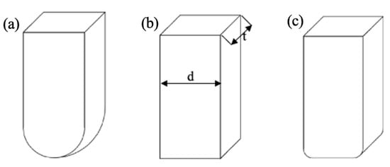
Figure 3.
Shape and dimensions of indenters used: (a) WS—spherical indenter, (b) WP—flat indenter, (c) WZ—rounded indenter.
A cuboid measuring 90 × 32 × 8 mm was taken as the test specimen, which was assigned liver parameters for two different models of viscoplastic material by Ogden and Yeoh. Based on a literature review of studies conducted by Nave and Carter, among others, Young’s modulus values for liver were obtained [18,19]. The value of this parameter depended on the source used and the gender of the patient. The results are shown in Table 4.
Table 4.
Mechanical parameters of the liver.
In order to represent ideal pressing, the two lateral planes were blocked in such a way that only translation (displacement) along the vertical plane was possible. Numerical simulations were carried out for the proposed three different penetrator shapes, which were assigned the material constants of steel in the elastic range (Table 5). Hex type elements sized at 0.5 mm were used for all components so that, on contact, the size of the elements would be the same. A demonstration of the geometry of the simulated flat penetrator is shown in Figure 4.
Table 5.
Steel material constants.
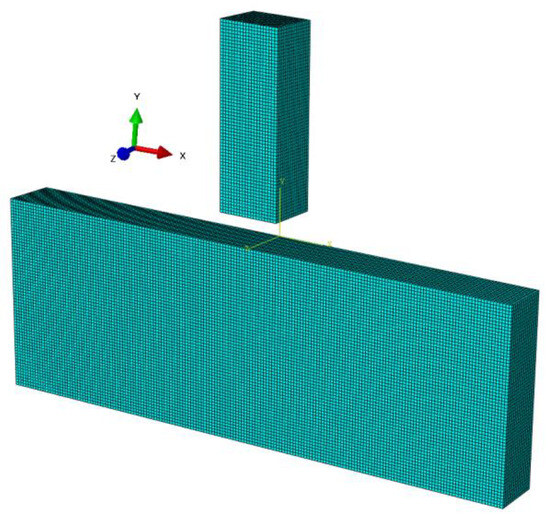
Figure 4.
Discretization of the system adopted for calculations.
Model scaling was performed by running a series of simulations for a duration of 8 s. An example of simulation runs for the Yeoh model is shown in Figure 5.
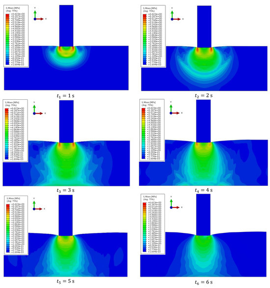
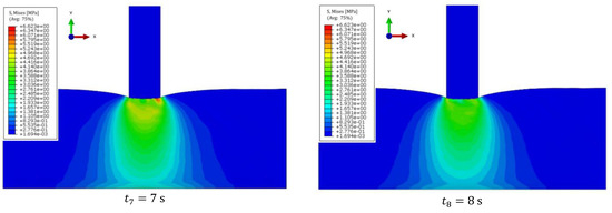
Figure 5.
Results for material data of Sample 1.
The values of deformation and stress occurring on the tested surface were analyzed. Figure 6 summarizes the results of the S12 stress in MPa for the four parameters of the Yeoh model.
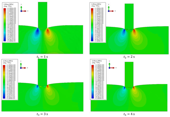
Figure 6.
Results of Yeoh’s parameter analysis.
From the numerical analyses carried out for various indenters, no significant differences were observed in the results obtained related to the mathematical model used. The difference between the results is 5%, which can be considered a very good fit. Larger differences were observed in the parameters of the constants that were used during the calculations. The individual results for different material constants are in the range of ±32%, which may indicate a satisfactory fit. This may be due to the large discrepancy in the initial data of the rheological models. The above results were used in the following numerical simulations.
4.2. Soft Structures
The skin consists of three layers: the epidermis, dermis, and subcutaneous dermis [20]. The outermost layer of the epidermis acts as a skin barrier.
Pereira [21] considers the skin to be a viscoelastic material in which there is a dynamic change in the stress–strain relationship until a steady state is reached [22]. The stress-related behavior of skin is usually described through three phases. When stressed up to 0.3%, elastin fibers offer low resistance to applied strain [23]. The skin exhibits isotropic behavior, with collagen fibers remaining tangled and intertwined with each other and not contributing to stiffness. Phase 1 offers a linear stress–strain relationship and low Young’s modulus (0.1–2.0 MPa) [10]. In Phase 2, the collagen fibers put up some strain resistance [24], and the crimped collagen fibers begin to stretch, thus introducing nonlinearity into the stress–strain relationship. In Phase 3, the final stage, for an applied strain above 0.6%, the notchiness begins to disappear and a linear stress–strain relationship can be observed. Collagen fibers break when a final tensile strain of 0.7% is applied [10].
Young’s modulus measurements vary according to a number of factors, including the type of test performed (in vivo or in vitro), the test method (tensile or compression), test speeds (in tensile testing), and the depth (in compression techniques). The collected data of stiffness modulus values depending on the referent are shown in Table 6. The skin was found to be highly anisotropic and viscoelastic, with a range of Young’s modulus from 5 kPa to 140 MPa.
Table 6.
Example Young’s modulus data for selected sections of leather.
The stress–strain relationship of most soft tissues can be simply characterized by three areas. At low stress, there is an area of relatively low elastic modulus, where large elongations can occur with little increase in stress. At high stresses, below the ultimate strength of the tissue, there is an area of high elastic modulus, where elongations are much smaller for a given increment of stress. The elastic properties in both of these areas are approximately linear, and it is, in principle, possible to derive elastic modulus values from the slope of the stress–strain response in each of these quasi-linear areas. Viidik called the slope of the high stress region elastic stiffness to distinguish it from the elastic properties of the tissue in the region at low stress [30]. In the middle region, there is a constant change in the gradient of the stress–strain relationship. According to Yamada’s study, for some tissues, one or both quasi-linear regions are absent; for others, the change from low modulus to high modulus occurs over a relatively small range of applied stress [31].
4.3. Hard Structures
At this stage, the component of the rib was modeled with the separation of the outer compact part and the inner spongy part. Table 7 and Table 8 show the mechanical parameters necessary to develop numerical models of the mentioned parts. The compact entity was modeled using the finite element method (FEM), while for the internal spongy structure, due to its biological–mechanical nature, it was decided to model the structure using the smooth particle hydrodynamics–finite element method (SPH/FEM).
Table 7.
Mechanical parameters of the cortical bone material.
Table 8.
Mechanical parameters of the spongy bone material.
The average length of a rib for adult humans is between 200 and 300 mm, and its width/depth usually oscillates between 25 and 50 mm. These measurements were taken along the curved length of the rib [32]. For the purposes of the study, these values were averaged over most of the population. Discretization was assumed at 0.5 mm using Tetra-type elements. Figure 7 shows the modeled rib. The numerical analysis performed is intended to represent a patient study, so factors such as material strengthening due to deformation or temperature effects were ignored.
Figure 7.
Preliminary layout for propagation analysis in bone: (a) geometry, (b,c) discretization.
The Johnson–Cook rheological model was used to describe the nature of the stress–strain mechanical properties of bone. This is a rheological model for describing elastic–plastic materials with nonlinear strengthening. The apparent linear nature of the material’s response to a given load in the first part is described by the elastic range using Young’s modulus and Poisson’s ratio. Then, once this limit is exceeded, nonlinear strengthening of the material is visible, for which the Johnson–Cook mathematical model is responsible in the numerical analysis. The Johnson–Cook model is a function of von Mises flow stress according to deformational strengthening, strain rate strengthening, and thermal softening. The equation below represents the Johnson–Cook model. The temperature and strain-rate strengthening effects are omitted from the analysis, omitting the second and third parts of the equation.
Here, A, B, C, n, and m are the material constants; is the melting point; is the initial temperature; ε is the plastic strain; is the plastic strain rate; and is the reference strain rate.
Through perpendicular application of the wave source, the displacements occurring depending on the time steps were analyzed. Figure 8 shows example values of this parameter for six time steps. For the description of the phenomenon, it was decided to use gray tones due to the better representation of the wavefront.
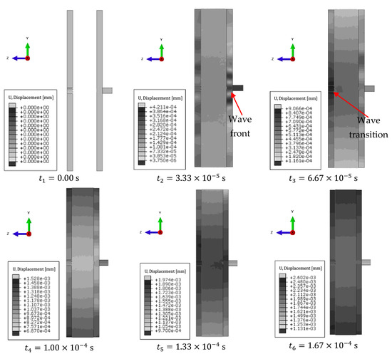
Figure 8.
Individual time steps for 3 MHz excitation.
The first time step illustrates the system without excitation. There is a visible wave front, with darker areas propagating through the area of higher stiffness first and then a weaker wave in the spongy part of the bone. The higher the stiffness—a higher value of Young’s modulus—the higher the speed of wave propagation in the object. At this stage, absorption of the forced wave in the spongy part of the bone can be observed.
4.4. Applied Final Model of the Tissue System
The developed models of components such as rib bones (distinguishing between the compact and spongy parts), muscles, adipose tissue, and the liver itself were put together [33]. In the final stage, a simplified geometric model was developed (Figure 9), which was eventually adapted for further numerical analysis and validated using the Computerized Imaging Reference Systems (CIRS) Model 039 calibrator.
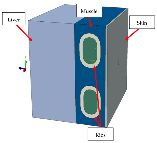
Figure 9.
Adopted model for the numerical analysis.
In the numerical simulations, the soft tissues and liver were modeled with 0.5 mm Hex elements. The rib bones with the separation of the external compact part were modeled using the FEM method. The internal spongy part was modeled using SPH-type elements. Discretization was assumed at 0.5 mm with the use of Tetra-type elements. The indenter was modeled using the Johnson–Cook model with material parameters for steel in the elastic range.
For a simplified model imitating liver, muscle, ribs, and skin, numerical simulations were performed in the frequency range of 1.0–5.0 MHz and with a liver stiffness of 1.5–12.5 kPa, as well as steatosis below 300 dB/m. Example results for forcing a vibration pulse at 3.0 MHz are shown in the Figure 10. The duration was determined to avoid imaging the reflection of the wave from the end of the liver, since the other organs were not included in the model. The time steps were chosen to avoid imaging wave reflection from the end of the system.
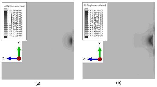
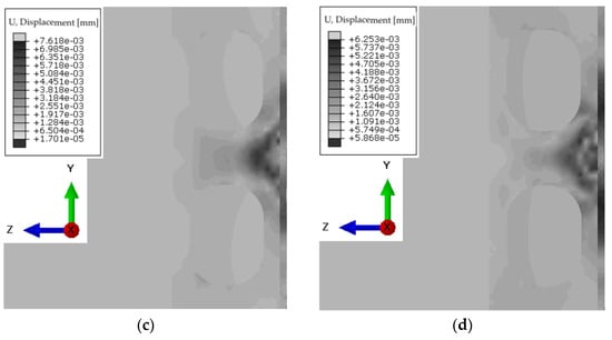
Figure 10.
Displacement of the wave front for the system at time steps: (a) 2.5 × 10⁻⁴ s; (b) 5.0 × 10⁻⁴ s; (c) 7.5 × 10⁻⁴ s; (d) 10.0 × 10⁻⁴ s.
The propagation of the longitudinal wave associated with interference can be seen already at the level of the ribs. The duration was determined to avoid imaging the reflection of the wave from the end of the liver, since the other organs were not included in the model.
4.5. Head Attachments
The stress–strain relationship of hyperelastic materials, such as silicone rubber, is usually defined as nonlinear, elastic, and incompressible [34]. In this study, a static compressive load test was performed for Smooth-On Ecoflex 00–20, which is the silicone rubber used in the experiment. The resulting curve in the stress–strain graph was nonlinear, indicating that the stiffness of this silicone material increases with the applied load.
In order to correlate the stress level with the change in stiffness of silicone, the stress–strain relationship obtained from the test was fitted to a quadratic curve, which can be described by Equation (8). The stresses at each load increment in the experiment were used to calculate the corresponding strains using Equation (8).
Here, is stress and is strain.
The resulting strain values were used to obtain the corresponding stiffness as the slope of the square curve at each stress level. Table 9 shows the stress and strain values at each load increment. Figure 11 shows this relationship for Smooth-On Ecoflex 00–20 in graphic form.
Table 9.
Material constants of the synthetic materials used to make the attachments [34].
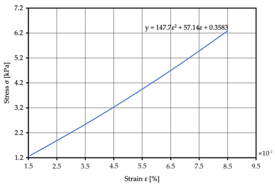
Figure 11.
Stress–strain relation for Smooth-On Ecoflex 00–20 under static compressive loading.
Figure 12 shows the two developed geometric shapes of the attachments: cylindrical and conical. To facilitate further analysis, the designations E_15 and D_0 are used. The distinctive feature of the proposed geometries was an indentation in the form of a ring at the top of the base for the measuring head of the FibroScan® device. The elements were discretized at the 0.5 mm level using Tetra-type elements. The assigned values of material constants were taken from previous in-house studies and from the manufacturer’s website.
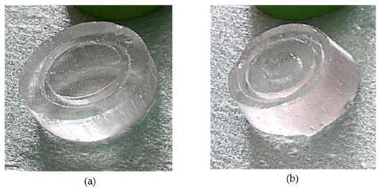
Figure 12.
Physical models of the developed attachments with specific shapes: (a) cylindrical E_15, (b) conical D_0.
Numerical analysis was performed for two geometric shapes of attachments and three types of material: Ecoflex 00–20, Medical Gel #0, and Agar Progel at forcing frequencies ranging from 1.0–5.0 MHz.
Figure 13 and Figure 14 show the different simulation time steps for wavefront propagation at 3 MHz using a cylindrical and a conical attachment made of Ecoflex 00–20. Table 10 shows a summary of these results for Ecoflex 00–20. Table 11 and Table 12 show the results of material Medical Gel #0 and Agar Progel, sequentially.
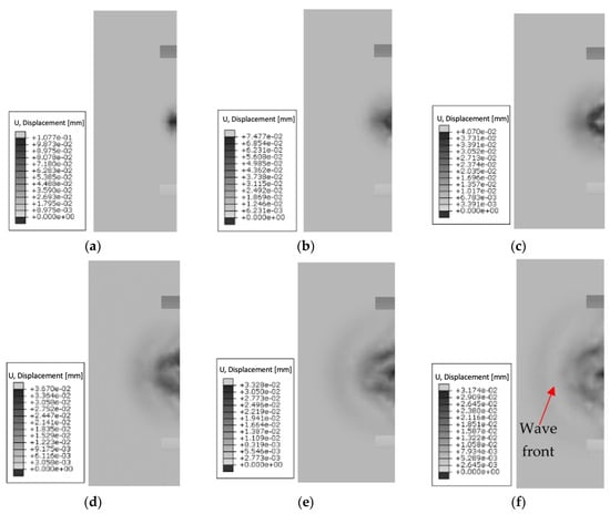
Figure 13.
Summary of wave propagation using a cylindrical head at 3 MHz over time: (a) 1.6 × 10⁻⁴ s; (b) 3.3 × 10⁻⁴ s; (c) 5 × 10⁻⁴ s; (d) 6.6 × 10⁻⁴ s; (e) 8.3 × 10⁻⁴ s; (f) 1.0 × 10⁻³ s.
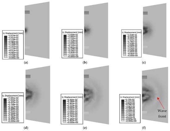
Figure 14.
Summary of wave propagation using a conical head at 3 MHz over time: (a) 1.6 × 10⁻⁴ s; (b) 3.3 × 10⁻⁴ s; (c) 5.0 × 10⁻⁴ s; (d) 6.6 × 10⁻⁴ s; (e) 8.3 × 10⁻⁴ s; (f) 1.0 × 10⁻³ s.
Table 10.
Summary of results for cylindrical and conical heads made of Ecoflex 00–20 material.
Table 11.
Summary of results for cylindrical and conical heads made of Medical Gel #0 material.
Table 12.
Summary of results for cylindrical and conical heads made of Agar Progel material.
A mechanical wave generated using a cylindrical head at a frequency of 3 MHz gradually propagates in the medium, and its amplitude decreases with time (e.g., for the first time step of 0.00016 s, the maximum displacement is 0.11 mm, and for the last 0.001 s, it has a value of 0.03 mm). It propagates along the axis of the cylinder. At 0.00016 s, the wave is at a relatively early stage of propagation. It moves along the head of the cylinder, propagating through the medium as a longitudinal wave. As it passes, the wave gradually propagates through the medium and moves away from the source. For the last time step of 0.001 s, the wavefront propagates a long distance from the cylindrical head. Its amplitude is significantly reduced and the wave energy further diffuses in the medium. The cylindrical shape of the head used has a direct effect on the stiffness, in turn affecting the depth of wave propagation.
The phenomenon of wave propagation depends on the shape of the head. The conical head is a geometrical form through which it is possible to focus or scatter a wave. For the phenomenon under study, at a time step of 0.00016 s, an early stage of wave propagation from the head is observed. The area in which the wave occurs is limited and does not propagate to larger distances. As time progresses, the shape of the head used allows observation of wave dispersion inside the medium. For the last time step of 0.001 s, the area in which the wave is observable is the largest, but its intensity is weakened. For the first time step, a maximum displacement of 0.27 mm is observed, and for the last time step, it is 0.06 mm.
Results were summarized for the three materials in an arrangement of two attachment shapes. The results are shown in Figure 15.
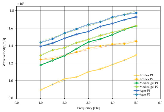
Figure 15.
Wave velocity combination diagram for different forcing frequencies.
The designation P1 indicates a cylindrical attachment, while P2 indicates a conical attachment. In addition, the trend line is plotted as a linear function. The discrepancies may be due to the contact between the inductor and the attachment and the reading of the wave velocity data for individual equal time steps. Only for the Ecoflex 00–20 material was a large discrepancy observed between the cylindrical and conical attachments, at 25%. This may be due to the stiffness of the geometric system itself—that is, the effect of shape on the stiffness of the component, given the same material constants. In other cases, the results converge, and their difference does not exceed 2.4% for Medical Gel #0 or 5.2% for Agar Progel, which indicates a very good fit.
5. Experimental Study Using Phantoms and Results
In order to pre-determine materials for measurement with the FibroScan® head, a series of tests were performed. Four CIRS Model 039 phantoms were used, all filled with Zerdine® gel but differing in Young’s modulus values (0.85 kPa, 6.67 kPa, 15.76 kPa, 32.49 kPa). The average ultrasound velocity for all phantoms was similar, at around 1538 m/s. A comparable level of contrast of the speckle imaging of the healthy liver was also maintained.
First, control measurements were performed, where the universal M-type (3.5 MHz) head of the FibroScan® device was applied directly to the foil-protected surface of the phantom. During the test, the measuring tip was mounted on a specially prepared tripod (Figure 16) so that a constant pressure force was maintained and its position was perpendicular to the phantom surface.
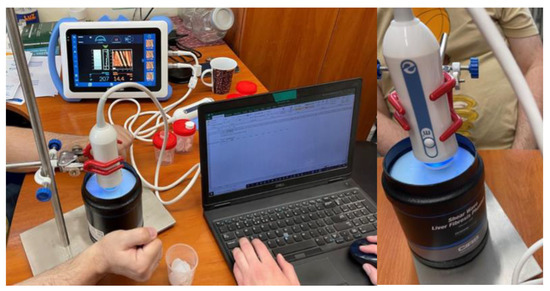
Figure 16.
The method of fixing the head for control measurements with the FibroScan® device.
This design made it possible to achieve satisfactory repeatability of results. Distilled water was used as a medium to ensure good mechano-acoustic coupling.
The study was carried out for four CIRS phantoms, but for the one characterized by the lowest Young’s modulus value (0.85 kPa), no measurement was possible. The FibroScan® device has a measurement range of 1.5–75.0 kPa, meaning it does not include the value for this model in its range. The results of the obtained elastic modulus and damping values for the other three phantoms are shown in Figure 17.
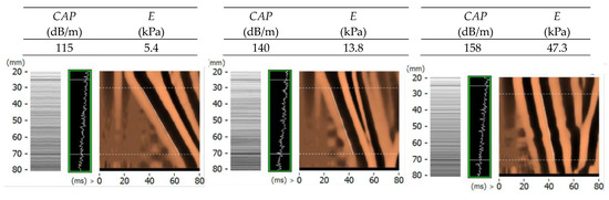
Figure 17.
Overview of transverse and ultrasonic wave propagation images recorded with the FibroScan® device for three phantoms from CIRS (fabric Young’s modulus: 6.67 kPa, 15.75 kPa, 32.49 kPa).
Analysis of the results obtained allows us to conclude that the results for the phantom with the lowest value of Young’s modulus of the three tested (6.67 kPa) were underestimated by about 19%. For the medium stiffness, the error oscillated around 12%, and for the highest stiffness, an overestimation of 47% was achieved. It was found that as the stiffness of the phantom increases, the spread of the results increases. The results obtained allowed the thesis that the thickness of the selected materials should be as small as possible, so that the unfavorable value of wave attenuation does not occur.
The next stage of the study was to check the commonly used materials allowing measurement with the FibroScan® device on CIRS phantoms. Samples were made of materials such as Agar Progel, Medical Gel #0, and Ecoflex 00–20 silicone rubber for later construction of overlays [15,16,17]. The prepared samples were placed between the head and the surface of the phantom, additionally protected by a film. Example photos of the realization of measurement tests of designed and fabricated attachments of different thicknesses on CIRS Model 039 phantoms using the FibroScan® apparatus are shown below (Figure 18).
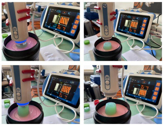
Figure 18.
Photos from the implementation of measurement tests of attachments of different thicknesses made of Agar Progel material on CIRS Model 039 phantoms using FibroScan®.
In order to evaluate the suitability of selected shapes and thicknesses of D_0 and E_15 attachments of Agar Progel, Medical Gel #0, and Ecoflex 00–20 materials, this chapter compares the average values of stiffness and ultrasound attenuation measurements of CIRS Model 039 phantoms E = 6.67 kPa and 15.75 kPa, as well as images of 50 Hz transverse wave propagation and a 3.5 MHz ultrasonic wave recorded with the FibroScan® device (Figure 19 and Figure 20).
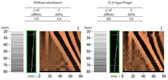
Figure 19.
A control summary of transverse and ultrasonic wave propagation images recorded with the Fibro-Scan® device in sample measurements of the CIRS Model 03 E = 6.67 kPa phantom without and with the use of D_0 attachments made of Agar Progel material.
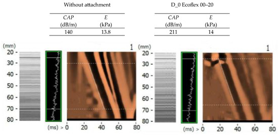
Figure 20.
A control summary of transverse and ultrasonic wave propagation images recorded with the Fibro-Scan® device in example measurements of the CIRS Model 03 E = 15.75 kPa phantom without and with the use of D_0 attachments made of Ecoflex material (without the insert and with the Fegura Sil silicone insert).
Analysis of control measurements of the target developed D_0 and E_15 attachments from all three target materials selected for testing (Agar Progel, Medical Gel #0, Ecoflex 00–20) confirms their correct performance as a mechanical–acoustic simulation of the intermediate layer between skin and liver tissue. The FibroScan® device is capable of making correct measurements of stiffness and ultrasound attenuation and visualizes good quality images of 50 Hz transverse wave propagation and 3.5 MHz ultrasound wave propagation in the tested CIRS Model 039 liver fibrosis phantoms, which is visible in comparison with measurements and images obtained without attachments and in comparison with studies of these phantoms available in the literature and performed additionally with elastography-enabled ultrasound equipment.
6. Discussion
Simulation results of the propagation of the mechanical wave deep into the studied system in the form of tissues, ribs, and liver show visible interference already at the level of the rib bones. In the simulation model used, further organs and time steps were omitted due to the effect of wave reflection from the end of the liver. Thus, the resulting wave effect was analyzed in detail in the frequency range of 1.0–5.0 MHz, with liver stiffness of 1.5–12.5 kPa and liver steatosis below 300 dB/m. The resulting figure represented the values of the speed of sound propagation in the analyzed medium. In this case, reference was made to an excitation frequency of 3.5 MHz, for which a value of 1569 m/s with a flat tip was obtained in numerical simulation. Validation of the speed of sound propagation on the CIRS Model 039 phantom using FibroScan® and the XL head was averaged as 1538 m/s from four measurements. The scatter of the results from the simulations and tests on the phantom oscillates at 2%, indicating the correctness of the simulations carried out.
The scanning head attachment was applied to the surface of three types of materials (Ecoflex 00–20, Medical Gel #0, Agar Progel), and the attenuation values and speed of wave propagation were obtained. The used value of the frequency of the inductor short-circuited in the range of 1.0–5.0 MHz. The study focused on obtaining correct values of wave propagation velocity close to biological tissues, where for fat the value is 1410 m/s and for muscle it is 1630 m/s. This action was intended to prevent mechanical damage caused by the passage of the wave through the organ. For the Ecoflex material, wave velocity results in the range of 800–1700 m/s for the conical and cylindrical overlay were obtained by numerical simulation. An underestimation of the lower limit of the results is observed for the Ecoflex 00–20 material, the use of which at low inductor frequencies can lead to measurement errors. For the Medical Gel #0 material, results were obtained in the range of 1128–1576 m/s, and for Agar Progel, the values oscillated in the range of 1341–1704 m/s. Comparing the results of the obtained wave propagation velocities for these two materials with those for biological media, a satisfactory match was found, which did not exceed a difference of 30%.
The analysis of measurements carried out using cylindrical and conical overlays for three selected materials (Agar Progel, Medical Gel #0, Ecoflex 00–20) for both numerical and experimental methods confirms the validity of the liver study in terms of mechanical–acoustic simulation. Comparing the results obtained on the CIRS Model 039 phantoms for the use of the attachment and its absence with the results reported in the literature [35], it can be concluded that the FibroScan® device allows adequate measurement of the stiffness and attenuation of ultrasound for liver examination.
7. Conclusions
Analysis of the results from the numerical analyses performed for spherical, flat, and rounded indenters allows us to conclude that there are no significant differences in the results obtained that could be related to the mathematical model used. For the adopted rheological models of Oghen and Yeoh, comparable results were obtained. Their differences oscillate at the level of 5%, which can be considered a very good fit. A greater divergence of results is observed in the parameters of material constants used for numerical calculations The differences obtained when changing the constants oscillate within ± 32%, which may indicate a satisfactory fit. This may be due to the large discrepancy in the initial data of the rheological models.
Measurement of the stiffness and attenuation of the ultrasound wave with the FibroScan® device carried out on the CIRS Model 039 phantoms allows us to conclude that the average measured values do not deviate from the manufacturer’s stated values. It was found that as the stiffness of the phantom increases, the scatter of the results increases. For all phantoms tested with attachments, attenuation values less than the limit value of 300 dB/m were recorded. The results obtained allowed the thesis that the thickness of the selected materials (Agar Progel, Medical Gel #0, Ecoflex 00–20) should be as small as possible so that the unfavorable value of wave attenuation does not occur.
The attenuation of ultrasound in the skin increases with frequency and averages a few to several dB/cm in the frequency range of 1.0–5.0 MHz. Too much attenuation in the attachment can weaken the ultrasound wave entering the liver tissue and introduce measurement errors or make measurements impossible. Durable gel- or rubber-like materials with ultrasound attenuation in the range of a few to several dB/cm are available.
The use of the Johnson–Cook elastic–plastic rheological model to describe bone tissue shows a very good fit for both the compact and spongy parts. At the same time, using the hybrid FEM/SPH method in this case shows a very good fit. The spongy structure of the bone is ideal for modeling with the SPH method. During the phenomenon of wave passage through the ribs, a wave front is observed, propagating first along the area of higher stiffness, in this case the cortical structure of the bone. Then, a weaker wavefront is seen in the spongy substance. It is concluded that there is a directly proportional relationship between stiffness and the speed of wave propagation. The higher the stiffness, and thus the higher the value of Young’s modulus, the higher the speed of wave propagation in the object. In addition, absorption of the forced wave in the spongy part of the bone is observed.
The presented results of the numerical analysis of the preliminary check of the efficiency in the propagation of a mechanical wave due to the application of the measuring part of the FibroScan® elastograph to the examined organ demonstrate the correctness of the assumed methodology. The result of the wave speed (1569 m/s) correlates with the value for a healthy liver (1550 m/s), which is a very good match.
Author Contributions
Data curation, K.K.; Formal analysis, K.R. and R.Ś.; Investigation, K.R. and K.O.; Methodology, D.P. and K.O.; Project administration, D.P. and R.Ś.; Resources, K.R. and R.Ś.; Supervision, K.J. and K.O.; Validation, D.P. and K.O.; Writing—original draft, K.K. and K.J.; Writing—review & editing, D.P., K.K. and K.J. All authors have read and agreed to the published version of the manuscript.
Funding
The work was carried out as part of the project POIR.01.01. 01-00-0462/21, co-financed by the European Regional Development Fund under the Smart Growth Operational Program 2014–2020.
Institutional Review Board Statement
Not applicable.
Informed Consent Statement
Not applicable.
Data Availability Statement
Data sharing is not applicable to this article. The data are owned by TIBA Ltd., and not publicly available.
Acknowledgments
Calculations have been carried out in Wroclaw Centre for Networking and Supercomputing (http://www.wcss.pl), grant No. 452.
Conflicts of Interest
Robert Śliwiński is co-owner of TIBA Ltd. and also co-author of the article. The views and opinions expressed in this paper are those of the authors and do not necessarily reflect the views or positions of TIBA Ltd.
References
- Milkiewicz, P. Elastografia Wątroby w Codziennej Praktyce Klinicznej/ Liver Elastography in Everyday Clinical Practice. Gastroenterol. Klin. 2017, 1, 1–6. [Google Scholar]
- Sánchez Antolin, G.; Garcia Pajares, F.; Vallecillo, M.A.; Fernandez Orcajo, P.; Gómez de la Cuesta, S.; Alcaide, N.; Gonzalez Sagrado, M.; Velicia, R.; Caro-Patón, A. FibroScan Evaluation of Liver Fibrosis in Liver Transplantation. Transplant. Proc. 2009, 41, 1044–1046. [Google Scholar] [CrossRef]
- Rajamani, A.S.; Rammohan, A.; Sai, V.V.R.; Rela, M. Current Techniques and Future Trends in the Diagnosis of Hepatic Steatosis in Liver Donors: A Review. J. Liver Transplant. 2022, 7, 100091. [Google Scholar] [CrossRef]
- Malik, R.; Afdhal, N. Stiffness and Impedance: The New Liver Biomarkers. Clin. Gastroenterol. Hepatol. 2007, 5, 1144–1146. [Google Scholar] [CrossRef]
- Castera, L.; Forns, X.; Alberti, A. Non-Invasive Evaluation of Liver Fibrosis Using Transient Elastography. J. Hepatol. 2008, 48, 835–847. [Google Scholar] [CrossRef]
- Zenovia, S.; Stanciu, C.; Sfarti, C.; Singeap, A.M.; Cojocariu, C.; Girleanu, I.; Dimache, M.; Chiriac, S.; Muzica, C.M.; Nastasa, R.; et al. Vibration-Controlled Transient Elastography and Controlled Attenuation Parameter for the Diagnosis of Liver Steatosis and Fibrosis in Patients with Nonalcoholic Fatty Liver Disease. Diagnostics 2021, 11, 787. [Google Scholar] [CrossRef]
- Ferraioli, G. Quantitative Assessment of Liver Steatosis Using Ultrasound Controlled Attenuation Parameter (Echosens). J. Med. Ultrason. 2021, 48, 489–495. [Google Scholar] [CrossRef]
- Opieliński, K.; Pruchnicki, P.; Świetlik, T. Analiza Parametrów Mechano-Akustycznych Skóry i Ewentualnie Innych Istotnych Pomiarowo Warstw Oraz Tkanki Wątroby; Raport z Badań (Materiały Niepublikowane); Politechnika Wrocławska: Wrocław, Poland, 2022. [Google Scholar]
- Bochenek, A. Anatomia Człowieka; PZWL: Warszwa, Poland, 1992; Volume 2. [Google Scholar]
- Holzapfel, G. Biomechanics of Soft Tissue. In Handbook of Material Behavior Nonlinear Models and Properties; LMT-Cachan; Academic Press: Graz, Austria, 2000. [Google Scholar]
- Shanahan, D. Patrick W. Tank and Thomas R. Gest, Atlas of Anatomy. Lippincott Williams & Wilkins, 2008. ISBN: 9780781785051. Clin. Anat. 2009, 22, 848. [Google Scholar] [CrossRef]
- Dwivedi, K.K.; Lakhani, P.; Kumar, S.; Kumar, N. A Hyperelastic Model to Capture the Mechanical Behaviour and Histological Aspects of the Soft Tissues. J. Mech. Behav. Biomed. Mater. 2022, 126, 105013. [Google Scholar] [CrossRef]
- Bergström, J. Linear Viscoelasticity. In Mechanics of Solid Polymers; William Andrew Publishing: Norwich, NY, USA, 2015; pp. 309–351. [Google Scholar] [CrossRef]
- Jung, W.; Li, J.; Chaudhuri, O.; Kim, T. Nonlinear Elastic and Inelastic Properties of Cells. J. Biomech. Eng. 2020, 142, 100806. [Google Scholar] [CrossRef]
- Surendran, G.; Sherje, A.P. Biomedical Applications of Agar and Its Composites: A Mini-Review. Nat. Prod. J. 2022, 13, 23–30. [Google Scholar] [CrossRef]
- Adusei, S.; Ternifi, R.; Fatemi, M.; Alizad, A. Custom-Made Flow Phantoms for Quantitative Ultrasound Microvessel Imaging. Ultrasonics 2023, 134, 107092. [Google Scholar] [CrossRef]
- Liao, Z.; Hossain, M.; Yao, X. Ecoflex Polymer of Different Shore Hardnesses: Experimental Investigations and Constitutive Modelling. Mech. Mater. 2020, 144, 103366. [Google Scholar] [CrossRef]
- Nava, A.; Mazza, E.; Furrer, M.; Villiger, P.; Reinhart, W.H. In Vivo Mechanical Characterization of Human Liver. Med. Image Anal. 2008, 12, 203–216. [Google Scholar] [CrossRef]
- Carter, F.J.; Frank, T.G.; Davies, P.J.; McLean, D.; Cuschieri, A. Measurements and Modelling of the Compliance of Human and Porcine Organs. Med. Image Anal. 2001, 5, 231–236. [Google Scholar] [CrossRef]
- Groves, R.B. Quantifying the Mechanical Properties of Skin In Vivo and Ex Vivo to Optimise Microneedle Device Design; Computer Methods in Biomechanics and Biomedical Engineering: London, UK, 2012. [Google Scholar]
- Pereira, B.P.; Lucas, P.W.; Swee-Hin, T. Ranking the Fracture Toughness of Thin Mammalian Soft Tissues Using the Scissors Cutting Test. J. Biomech. 1997, 30, 91–94. [Google Scholar] [CrossRef]
- Matsumura, H.; Yoshizawa, N.; Watanabe, K.; Vedder, N.B. Preconditioning of the Distal Portion of a Rat Random-Pattern Skin Flap. Br. J. Plast. Surg. 2001, 54, 58–61. [Google Scholar] [CrossRef]
- Oxlund, H.; Manschot, J.; Viidik, A. The Role of Elastin in the Mechanical Properties of Skin. J. Biomech. 1988, 21, 213–218. [Google Scholar] [CrossRef]
- Silver, F.H.; Freeman, J.W.; Devore, D. Viscoelastic Properties of Human Skin and Processed Dermis. Skin. Res. Technol. 2001, 7, 18–23. [Google Scholar] [CrossRef]
- Zheng, Y.; Mak, A.F.T. Effective Elastic Properties for Lower Limb Soft Tissues from Manual Indentation Experiment. IEEE Trans. Rehabil. Eng. 1999, 7, 257–267. [Google Scholar] [CrossRef]
- Khaothong, K. In Vivo Measurements of the Mechanical Properties of Human Skin and Muscle by Inverse Finite Element Method Combined with the Indentation Test. In Proceedings of the 6th World Congress of Biomechanics (WCB 2010), Singapore, 1–6 August 2010; IFMBE Proceedings. Springer: Berlin/Heidelberg, Germany; pp. 1467–1470. [Google Scholar] [CrossRef]
- Boyer, G.; Zahouani, H.; Le Bot, A.; Laquieze, L. In Vivo Characterization of Viscoelastic Properties of Human Skin Using Dynamic Micro-Indentation. In Proceedings of the Annual International Conference of the IEEE Engineering in Medicine and Biology Society, Lyon, France, 22–26 August 2007; pp. 4584–4587. [Google Scholar] [CrossRef]
- Boyer, G.; Laquièze, L.; Le Bot, A.; Laquièze, S.; Zahouani, H. Dynamic Indentation on Human Skin in Vivo: Ageing Effects. Skin. Res. Technol. 2009, 15, 55–67. [Google Scholar] [CrossRef] [PubMed]
- Boyer, G.; Pailler Mattei, C.; Molimard, J.; Pericoi, M.; Laquieze, S.; Zahouani, H. Non Contact Method for in Vivo Assessment of Skin Mechanical Properties for Assessing Effect of Ageing. Med. Eng. Phys. 2012, 34, 172–178. [Google Scholar] [CrossRef] [PubMed]
- Viidik, A. Properties of Tendons and Ligaments. In Handbook of Bioengineering; McGraw-Hill: New York, NY, USA, 1987. [Google Scholar]
- Yamada, H. Strength of Biological Materials; Robert E. Krieger Publishing Co.: New York, NY, USA, 1973. [Google Scholar]
- Dansereau, J.; Stokes, I.A.F. Measurements of the Three-Dimensional Shape of the Rib Cage. J. Biomech. 1988, 21, 893–901. [Google Scholar] [CrossRef] [PubMed]
- Mazurkiewicz, K.; Sybilski, Ł.; Małachowski, K.; Pietró, K.; Mazurkiewicz, Ł.; Sybilski, K.; Małachowski, J. Correlation of Bone Material Model Using Voxel Mesh and Parametric Optimization. Materials 2022, 15, 5163. [Google Scholar] [CrossRef]
- Liu, C.; Zhuang, Y.; Nasrollahi, A.; Lu, L.; Haider, M.F.; Chang, F.K. Static Tactile Sensing for a Robotic Electronic Skin via an Electromechanical Impedance-Based Approach. Sensors 2020, 20, 2830. [Google Scholar] [CrossRef] [PubMed]
- Mulabecirovic, A.; Mjelle, A.B.; Gilja, O.H.; Vesterhus, M.; Havre, R.F. Repeatability of Shear Wave Elastography in Liver Fibrosis Phantoms—Evaluation of Five Different Systems. PLoS ONE 2018, 13, e0189671. [Google Scholar] [CrossRef]
Disclaimer/Publisher’s Note: The statements, opinions and data contained in all publications are solely those of the individual author(s) and contributor(s) and not of MDPI and/or the editor(s). MDPI and/or the editor(s) disclaim responsibility for any injury to people or property resulting from any ideas, methods, instructions or products referred to in the content. |
© 2023 by the authors. Licensee MDPI, Basel, Switzerland. This article is an open access article distributed under the terms and conditions of the Creative Commons Attribution (CC BY) license (https://creativecommons.org/licenses/by/4.0/).