Abstract
Super-resolution enhances the spatial resolution of remote sensing images, yielding clearer data for diverse satellite applications. However, existing methods often lose true detail and produce pseudo-detail in reconstructed images due to an insufficient number of ground truth images for supervision. To address this issue, a prediction-to-prediction super-resolution (P2P-SR) network under a multi-level supervision paradigm was proposed. First, a multi-level supervision network structure was proposed to increase the number of supervisions by introducing more ground truth images, which made the network always predict the next level based on the super-resolution reconstruction results of the previous level. Second, a super-resolution component combining a convolutional neural network and Transformer was designed with a flexible super-resolution scale factor to facilitate the construction of multi-level supervision networks. Finally, a method of dividing the super-resolution overall scale factor was proposed, enabling an investigation into the impact of diverse numbers of components and different scale factors of components on the performance of the multi-level supervision network. Additionally, a new remote sensing dataset containing worldwide scenes was also constructed for the super-resolution task in this paper. The experiment results on three datasets demonstrated that our P2P-SR network outperformed the state-of-the-art (SOTA) methods.
1. Introduction
Super-resolution improved image resolution and enhanced the accuracy of image processing tasks such as target detection, semantic segmentation, and scene classification [1,2,3]. Applying super resolution to remote sensing could provide high-resolution datasets [4,5,6,7,8] for land planning, environmental protection, and disaster prediction [9,10,11]. In recent years, an increasing number of remote sensing satellites have been launched into orbit, and the imaging resolution of remote sensing satellites has been rising. This provides a wealth of training data for the super resolution of remote sensing images.
Since deep networks were introduced to super-resolution techniques, various methods based on different backbone networks have been proposed one after another [12,13,14,15,16]. In these studies, several authors discussed the ill-posedness of super resolution [17,18,19,20]. The same low-resolution image can be obtained by downsampling several different high-resolution images. As an inverse process of downsampling, super resolution predicts multiple high-resolution images from the same one low-resolution image and selects the high-resolution image that is most similar to the ground truth. Therefore, super resolution is an ill-posed problem. The space of all possible functions for mapping from a low-resolution image to high-resolution images is large. This poses difficulties in training super-resolution networks and limits the network’s performance improvement. Consequently, reducing the ill-posedness of super resolution has become a significant research issue in the development of this technique.
The VDSR-based super-resolution method [17] was one of the first proposed to reduce the ill-posedness of super resolution. In [17], it was noted that the limited number of layers in the feature extraction module of SRCNN restricted detail recovery in super-resolution output. VDSR effectively improved super-resolution performance by deepening the network to expand the receptive field. However, the number of layers in the current deep network is generally large, and the transformer structure further expands the receptive field of feature extraction. Therefore, simply deepening the network no longer reduces the ill-posedness of super resolution. In [20], the ill-posedness of super resolution was analyzed mathematically. The large space of possible functions for mapping from low-resolution images to high-resolution images makes it difficult to accurately fit a mapping function using a deep network. To increase the constraints of super-resolution networks, a dual regression network was proposed. This network introduced additional supervision during training by comparing super-resolution results with high-resolution ground truth and computing a loss function between the downsampled result image and the input image. This method effectively reduced the space of possible mapping functions.
The dual regression network increased the number of supervisions from one to two, which increased the constraints in the super-resolution process and reduced the ill-posedness of super resolution. However, the second supervision was applied to the downsampled output image, potentially losing the recovered image detail again during the downsampling process. Moreover, the loss function computed between low-resolution images might be unsuitable for evaluating the super-resolution performance of the network. To further reduce the ill-posedness of super resolution, a Prediction-to-Prediction Super-Resolution (P2P-SR) network under a multi-level supervision paradigm was proposed. Unlike the conventional one-step or dual regression super resolution, our method utilized multiple Basic Super-Resolution Components (BSRC) with smaller scale factors for image reconstruction. Supervisions were applied at the output of each component, introducing multiple levels of constraints to the super-resolution process.
To reduce the ill-posedness of super resolution, a progressive super-resolution network based on multi-level supervision was proposed. The contribution of our approach is as follows.
- (1)
- A multi-level supervision structure was proposed and multi-level supervision images were applied to the output of each component to increase the guidance in the super-resolution progress and reduce the ill-posedness.
- (2)
- A basic super-resolution component with adjustable scale factor was designed to enable the construction of different multi-level supervision network-like building blocks.
- (3)
- In the progressive structure, both the number of components and the scale factor of each component had an impact on the performance of the network. A method for dividing the super-resolution overall scale factor was proposed to obtain the best combination of BSRCs.
The multi-level supervision super-resolution network based on the best BSRC combination was compared with existing SOTA methods. The experimental results demonstrated that our method was effective in improving the super-resolution performance.
2. Related Work
Super resolution was initially introduced and applied to natural images before being adapted and employed for remote sensing images. Over time, various super-resolution techniques based on convolutional neural networks, generative adversarial networks, and Transformer structures were developed. Due to the ill-posedness of super resolution, increased attention has been given to this aspect as the scale factor of the proposed super-resolution methods increased. One effective approach to reduce the ill-posedness of the super-resolution problem is to increase supervision in the network training process. Consequently, several super-resolution methods aimed at increasing the number of supervisions were proposed, with some employing progressive structures, and others using loops or other structures. All these approaches enhanced the performance of super-resolution networks.
2.1. Super-Resolution Methods
As the most classical image processing network, convolutional neural networks were first introduced to super-resolution tasks in SRCNN [21]. SRCNN consisted of three convolutional layers, achieving image super resolution in a pre-upsampling and lightweight structure. The input data were upsampled before being sent into the network. However, the three-layer convolutional network lacked sufficient depth to extract deep image features. To address this issue, a very deep convolutional super-resolution network (VDSR) with 20 weight layers was proposed in [17]. The increase in the number of network layers significantly improved the network’s ability to extract image textures and super-resolution performance. The residual structure was introduced to super-resolution networks in [22], making it possible to further deepen the network depth. Super-resolution networks generally consist of two parts: feature extraction and image reconstruction. The above method improved the feature extraction performance by increasing the convolutional network depth. To improve the image reconstruction process, a new sub-pixel convolution structure was proposed in [23], replacing the traditional interpolation method. Experiment results evidenced that the sub-pixel convolution improved the super-resolution network performance and speed. However, it was difficult for sub-pixel convolution to be applied to non-integer multiples of super resolution. In [24], a post-upsampling super-resolution network structure was proposed. Most of the current super-resolution methods have adopted this post-upsampling structure.
Since its introduction, the transformer network has outperformed classical convolutional networks in various computer vision tasks. Compared with convolutional networks, the transformer network has a larger perceptual field and is more suitable for extracting global features of images. In recent years, the transformer has also been used in the field of super resolution. An image processing transformer [25] was proposed for low-level computer vision tasks, including denoising, super resolution, and so on. Based on the Swin Transformer, the SwinIR [26] network was proposed for super resolution. SwinIR uses both convolutional networks and Transformer to extract image features, improving performance while achieving a degree of lightweighting. The recently proposed ESRT [27] uses a combination of convolutional networks and transformers, and has made further efforts in network lightweighting.
With the advancements in the super resolution of natural images, various methods have been applied to remote sensing images. In [28], SRCNN was utilized for multispectral remote sensing image super resolution, unveiling research on remote sensing image super resolution. In [29], SRCNN and VDSR were applied to the single-frame super resolution of remote sensing images. An intensity hue saturation transform was used on the input image to speed up the network computation while preserving the color information. A local–global combined network (LGCNet) was proposed in [30]. It could learn multilevel representations of remote sensing images, including both local details and global environmental priors with its multifork structure. In [31], a deep distillation recursive network (DDRN) was proposed that contained more linking nodes with the same convolution layers and performed feature distillation and compensation in different stages of the network. Remote sensing image super-resolution methods basically followed the development of natural image super resolution. Recently, various Transformer-based backbone networks have also been applied to the super resolution of remote sensing images [32,33,34]. In [35], a transformer-based enhancement network was proposed to enhance the high-dimensional feature representation.
2.2. The Ill-Posedness of Super Resolution
The development of super-resolution methods has always been accompanied by the discussion of the ill-posedness of super resolution. In [17], the smaller receptive fields of convolutional networks were thought to worsen the ill-posedness of super resolution. The convolutional neural networks used for super resolution at that time had fewer layers and smaller network receptive fields. Local information contained by small patches was insufficient to recover image detail. The VDSR proposed in [7] used a deeper convolutional network to increase the perceptual field, using the information contained in the larger patches for image-detail recovery. The performance improvement was significant compared to SRCNN, which has fewer layers. With the rapid development of deep networks, the network depth and number of parameters increased dramatically. The Transformer for vision tasks expanded the field of perception even further to the entire image. Therefore, it is no longer appropriate to reduce the ill-posedness of super resolution by deepening the network. As the first application of GAN to super resolution, reducing the ill-posedness of super resolution was the main motivation of this work [36]. In [36], the researchers considered that multiple different super-resolution images could be reconstructed from the same low-resolution image. Pixel-wise loss functions such as MSE, which were commonly used at the time, were considered to be averaging over all super-resolution images. This resulted in over-smoothing of the image and loss of image detail. Therefore, a GAN-based super-resolution network was proposed to drive the super-resolution results towards a perceptually more convincing solution. Both of these methods were effective in improving the performance of super-resolution networks, but unfortunately the relationship between ill-posedness and network constraints was not discussed.
Multiple different high-resolution images can be downsampled to the same low-resolution image. In turn, multiple different super-resolution images can be reconstructed from the same low-resolution image. The task of super resolution is to select the closest one of these super-resolution images to the ground truth. In SRFlow [18], a super-resolution method based on normalized flow was proposed to learn the conditional distribution of the output. SRFlow therefore directly accounted for the ill-posedness of the problem and learned to predict diverse photo-realistic high-resolution images. In [10], the ill-posedness of super resolution was reduced from another perspective. Super resolution was considered to be the process of fitting a mapping function from a low-resolution image to a high-resolution image. Due to the ill-posedness of super resolution, the space of all possible mapping functions is huge. This makes it difficult to train the network. In order to address this issue, a dual regression network (DRN) [20] was proposed. During the training process of the DRN, the super-resolution image was reconstructed from the low-resolution input image, and the loss between it and the ground truth was calculated. The super-resolution image was then downsampled to the same size as the input image and compared to the input image, and another loss was calculated. The essence of DRN is the increase in the number of network supervisions. The increase in supervision benefits the introduction of more ground truth and imposes more constraints on the network. The improved performance of super-resolution networks due to DRN illustrated the effectiveness of increased supervision in reducing the ill-posedness of super resolution.
2.3. Progressive Structure for Super Resolution
Among the many image super-resolution methods, some researchers have also proposed the idea of progressive super resolution. Nevertheless, there were still some shortcomings in these methods. In [37], a progressive cascading residual network was proposed in response to the instability of network training. First, a super-resolution module with a magnification of two was trained, and then a new two-times super-resolution network was connected to it for training. A total of three such modules were trained and finally connected together to complete the eight-times super resolution. The results showed that this property yielded a large performance gain compared to the non-progressive learning methods. This method used the idea of progressive training, but did not use multiple levels of supervision. During the training of each module, only one supervision was used to evaluate the performance of the whole network. It still suffered from the problem of insufficient constraints. A leveraging multi-scale backbone with multi-level supervision [38] was proposed for thermal image super resolution. A total of five times supervision was performed for feature maps, feature fusion maps, and super-resolution results at different stages. Although the number of supervisions in this method was higher, most of the supervisions were applied to the feature map. The feature maps were visually quite different from a good super-resolution output image. In [35], a transformer-based multi-stage enhancement method was proposed for remote sensing image super resolution. An enhancement module was added after the super-resolution network to enrich the details. The super-resolution network was still a one-step approach, and the idea of a multi-stage approach was mainly reflected in the enhancement module.
3. Methods
3.1. Multi-Level Supervision Super-Resolution Network
As mentioned earlier, super resolution is a typically ill-posed problem. Its ill-posedness mainly comes from the huge space of all possible functions for mapping from low-resolution images to high-resolution images. Increasing the number of supervisions in the network can increase the constraints on the network training, gradually reduce the space of possible functions, and reduce the ill-posedness of super resolution. Most of the current super-resolution methods adopted a one-step supervision structure, which was only supervised once at the output of the super-resolution network, resulting in insufficient constraints in the super-resolution process. The unsuppressed ill-posedness of super resolution is visualized in the network output by the loss of image details and the appearance of pseudo-detail.
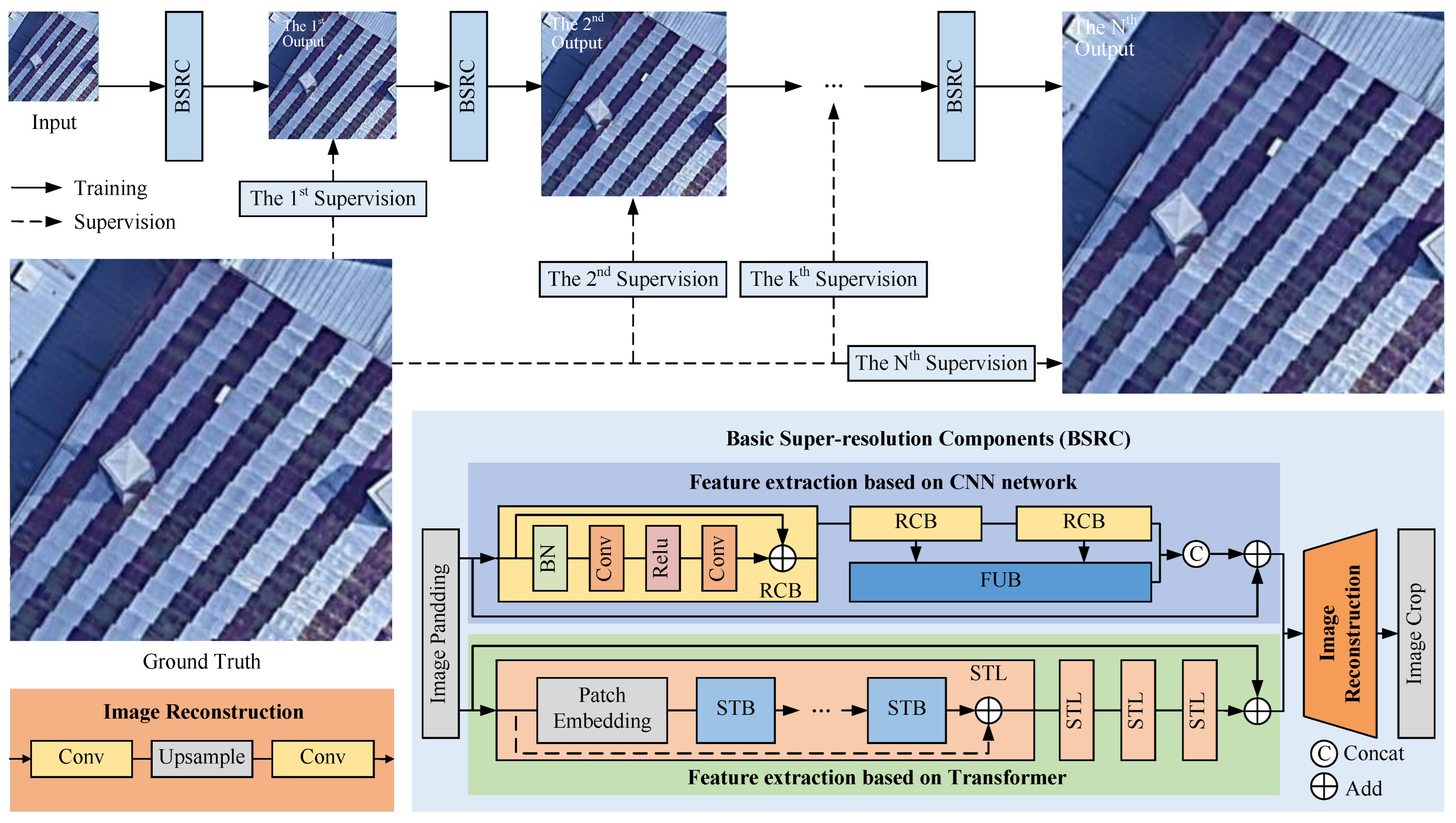
In order to reduce the ill-posedness of the super-resolution process and improve the super-resolution network performance, a progressive super-resolution network was proposed for remote sensing images based on multi-level supervision. As shown in Figure 1, the P2P-SR network consists of several basic super-resolution components and multi-level supervision. The overall super-resolution scalar factor of the P2P-SR network can be set flexibly. The BSRCs can be increased or decreased like building blocks, with fewer BSRCs for a smaller overall super-resolution scale factor and more BSRCs for a larger overall super-resolution scale factor. The scale factor of each BSRC is determined by the overall scale factor and the number of BSRCs. The BSRC consists of a multi-scale feature extraction module, a global feature extraction module, and an image reconstruction module. Considering that the scale factor of each BSRC should have some flexibility, the network structure of each BSRC is the same except for the image reconstruction module. This helps to shorten the overall training time of the network. During the network training, the training of the first BSRC was completed first. Its trained parameters were shared to the subsequent BSRCs, and all BSRCs were tuned together simultaneously to complete the overall network training. Our network used a progressive super-resolution structure and multi-level supervision. But this is not a simple stacking of network components. The cross-level loss functions were designed to facilitate better transfer of image detail loss across the network components. The effect of the number of BSRCs and each BSRC scale factor on network performance was explored when the overall scale factor was certain. These will be explained in detail in later sections.
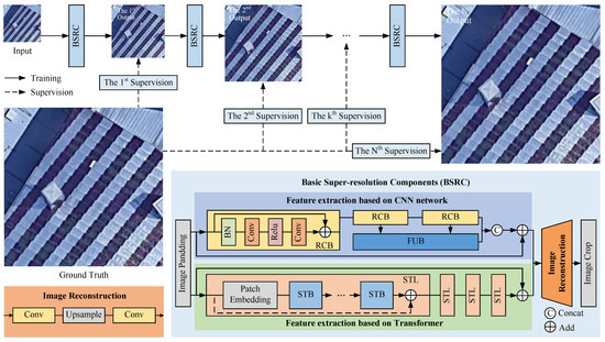
Figure 1.
The Prediction-to-Prediction Super-Resolution (P2P-SR) network consists of multiple Basic Super-Resolution Components (BSRC). The number of BSRCs and the scale factor of each BSRC can be flexibly adjusted.
To conveniently describe the multilevel supervision network, the overall scale factor was set to M, and the number of BSRCs was set to N. The P2P-SR net used N BSRC modules to accomplish M-times super resolution. At the output of each component, the super-resolution result was compared with the ground truth downsampled to the same size. The loss function was calculated between the result and the ground truth. The progressive super-resolution process of low-resolution remote sensing images can be expressed as
where I is the input low-resolution image, is the process of super resolution, is the loss function of the nth level, and and are adjustable weights. From Equation (1), it is clear that the multi-level supervision network aims to reduce the loss of each BSRC and the overall network loss at the same time. The loss of the Nth BSRC component is given a separate adjustable weight . This is because the Nth component is the last component of the network, and its output is also the output of the overall network. The output of the Nth component is evaluated not only by the loss function, but also by the visual perception of the human eye. Setting a separate weight for the loss function of the Nth level component helps to balance the network output between the evaluation metric and visual assessment.
The progressive super-resolution structure based on multi-level supervision is beneficial to improve the performance of the super-resolution network. On the one hand, the multi-level supervision structure introduces multi-level ground truth images and embeds new information of image details into the super-resolution process at the output of each BSRC. This helps to reduce the super-resolution ill-posedness and suppress the loss of detail or pseudo-detail in the super-resolution results. On the other hand, the progressive super-resolution structure reduces the number of pixels that each BSRC module needs to predict during the super-resolution process. For the classical one-step super-resolution method, the network needs to predict pixels from one pixel to complete the M-times super resolution. In our P2P-SR network, assuming the same scale factor for each BSRC, each BSRC only needs to predict pixels from one pixel. The number of pixels to be predicted is reduced, and the probability of pseudo-detail in the image is reduced. At the same time, the smaller the number of pixels to be predicted, the smaller the space of all possible functions for mapping from a low-resolution image to a high-resolution image. This can also be considered as reducing the ill-posedness of super resolution.
3.2. Basic Super-Resolution Component
Multiple basic super-resolution components form the main structure of P2P-SR. Each BSRC consists of multi-scale local feature extraction, global feature extraction and image reconstruction. Remote sensing images contain a rich variety and number of details of ground objects. The strong feature extraction capability is the basis for good super-resolution outputs. Both the CNN network and the transformer network were used for feature extraction in their network.
The feature extraction in our network consists of two parts: convolutional neural networks for extracting multi-scale local features and a transformer-based network for extracting global features. The global feature extraction was designed based on the Swin Transformer backbone. Based on Swin Transformer’s pyramidal backbone network, a plain backbone network was designed that was more suitable for super-resolution tasks. In parallel, the multi-scale local feature extraction is achieved by employing residual convolution blocks (RCB) and a feature-upsampling block (FUB). RCB comprises batch normalization, convolutional layers, and an activation function. Following RCB, the feature maps undergo a downsizing process, necessitating their upsampling through FUB before concatenation.
The residual structure was added at both the layer level and the block level. The residual structure of the layer level was designed to be optional. This is because it is considered that lightweight transformer networks tend to contain more layers in the 3rd block. The residual structure is more useful in the 3rd block than in the other blocks. A residual structure that can be chosen flexibly according to the number of layers in the block is beneficial for balancing network performance and lightweighting.
In the multi-scale local feature extraction part, RCB was designed to extract the multi-scale feature by the residual structure, and FUB was used to unify feature map resolution. The number of RCBs was set as 3, and a lightweight multi-scale feature map fusion structure was designed. The output feature map of the first RCB had the same size as the input image, and it was formulated as
where was the first RCB, was the input remote sensing images after image padding, and was the output of first RCB, Then, was sequentially fed into the two subsequent RCBs, and the feature map size was sequentially reduced by half. The outputs of the last 2 RCBs were fed to the FUB module for upsampling, and the results were formulated as
where was the FUB module. was defined as . , , and shared the same size and were concatenated by channel. The output of the local feature extraction branch was formulated as
Parallelly, 4 Swin transformer layers (STL) were set in the global feature extraction branch. The output of the ith STL was formulated as
where was the ith STL and the was the output of the ith STL. The output of the last STL was summed with . The output of the global feature extraction branch was formulated as
Finally, and was fed into the image reconstruction module, and the super-resolution result is formulated as
where is the image reconstruction module. Each BSRC magnified the image by a factor of . N was the number of BSRC, and M was the super-resolution multiplier of the P2P-SR network. Considering that may often be non-integer, the classical but flexible output size method of convolution layers and upsampling was used.
3.3. The Scale Factor Division Method
For the super-resolution process with a certain scale factor, a method was needed to divide the overall scale factor into each BSRC. As the number of BSRCs increases, the number of supervisions increases, and the super-resolution ill-posedness is reduced. At the same time, the total number of network layers increases, and the number of computations increases. The sum of super-resolution network performance and computational complexity can be formulated as
where is the high-resolution of the parameters of the nth BSRC, and and are the super-resolution output and the ground truth of the nth BSRC, respectively. and are vastly different in order of magnitude and need to be normalized before summing.
As seen from the above equation, the correlation between and the number of BSRCs n is difficult to predict. It may be assumed that the number of BSRCs increases from 1. Initially, the number of BSRCs is small, and with the network being sufficiently trained, the increase in the number of BSRCs benefits the increase in the number of supervisions in the network, which in turn helps to reduce the super-resolution ill-posedness. The reduction in super-resolution ill-posedness helps to reduce the probability of detail loss and pseudo-detail in the output image, which leads to a reduction in the of the nth BSRC. In this case, the increase in the number of BSRCs also leads to an increase in the number of network parameters. If the network is properly designed to be lightweight so that the increase of is smaller than the decrease of , then has the possibility to be reduced. In the comparison of experimental results, the performance improvement of our method on 4-times super-resolution results is more significant than 2 times, although 4-times super resolution requires more BSRCs. As the number of BSRCs continues to increase, the number of BSRCs may be saturated for a super-resolution task of certain scale factor. More BSRCs bring limited performance gains, but significantly increase the number of network parameters. Therefore, finding the appropriate number of BSRCs is important for our multi-level supervision-based super-resolution network.
After determining the number of BSRCs, the scale factor of each BSRC is also worth discussing. Let the number of BSRCs in the network be N and the ith BSRC super-resolution multiplier be , then the relationship between the number of BSRCs, the scale factor of each BSRC, and the overall scale factor of our super-resolution network is as follows:
From the above equation, it can be seen that when N increases, the scale factor of each component decreases. When N tends to infinity, tends to 1. This means that each BSRC only magnifies the input image at a very small factor. Each BSRC needs only a very small number of parameters to perform its own super-resolution task. Therefore, when N tends to infinity, the trend of increasing or decreasing the total number of parameters is difficult to predict. Therefore, it is necessary to optimize the BSRC combination and find out the relationship between super-resolution network performance, the number of parameters, and the scale-factor division method.
In the experiments on the various scale-factor division ways, it was proposed to start from two aspects, namely the number of BSRCs in the network and the super-resolution scale factor of each BSRC. In terms of the number of BSRCs, the higher the number of BSRCs, the more training constraints were introduced into the network, but the greater the computational complexity. The optimal number of BSRCs was obtained by comparing the super-resolution network performance and the computational complexity of different numbers of BSRCs. In terms of the scale factor of each BSRC, four combinations of isometric, isoperimetric, front-segment dense, and back-segment dense distributions were designed. The front-segment dense distribution and the back-segment dense distribution focused on the impact of early detail recovery and late detail recovery on the final super-resolution output, respectively. The isotropic and isoparametric distributions gave equal weight to early detail recovery and late detail recovery and were compared with each other. The super-resolution network performance and computational complexity of various combinations of scale factors were compared, and the optimal method to divide the overall scale factor was presented. The experimental results can be found in the subsection of ablation studies.
3.4. Loss Function
During the development of deep learning, various loss functions have been proposed. loss and perceptual loss [39] are the commonly used loss functions. loss can significantly improve the peak signal-to-noise ratio (PSNR) value of super-resolution results and is simple and effective to calculate. However, loss also has the problem of excessive smoothing, which is not conducive to the recovery of image details. For the progressive structure, different loss functions were used at different levels, and the losses at different levels were allowed to interact with each other.
Perceptual loss was used at the first and second BSRC, and a combination of perceptual loss and loss was used at the third and fourth BSRC. The loss function of the first and second BSRC can be formulated as
where is the perceptual loss and is a constant adjusted for training. This is because the recovery of image details relies heavily on the first two levels, and once a detail is lost somewhere, it is difficult to make up for it subsequently. Perceptual loss enables better control of detail loss by comparing the multi-scale feature map differences between the output and the ground truth. In the third and fourth BSRC, while controlling the loss of details, the output needs to match the human eye’s perception. Thus, the loss was added to the perceptual loss, and the sum can be formulated as:
where and are adjustable weights. The is used as part of the 3rd and 4th BSRC’s loss.
Due to our progressive structure and multi-level supervision, it is also necessary to consider the relationship between losses of multiple BSRCs. The loss of the 3rd and 4th BSRCs can be formulated as
As seen in the above equation, the loss of each BSRC includes the loss of the BSRCs before it. This is because the loss of detail in the output of the earlier BSRC will have an impact on the super-resolution performance of the subsequent BSRC. The penalty for the loss of detail in the earlier BSRC should be increased. It should also be noted that the weights of the losses in the previous BSRC are also different. The further the distance between two BSRCs, the larger the product of . A smaller weight should be given to the BSRC that is farther away as a balance.
4. Experiments
4.1. Dataset and Settings
Although there are a large number of remote sensing satellites operating in space, the remote sensing image datasets are far less complete than the set of natural images due to national security, data confidentiality, and other reasons. At the same time, existing remote sensing image datasets are not fully suitable for super-resolution tasks. On the one hand, most of them were made for target detection tasks. This has resulted in a limited variety of ground object detail contained in the images in the datasets. These datasets contained a large number of remotely sensed images of cars, aircraft, and boats, but lacked remotely sensed images of areas such as buildings, vegetation, and water surfaces. On the other hand, some datasets were produced in earlier years, and the limited resolution of remote sensing images made it difficult to provide effective supervision for super-resolution tasks. Therefore, a new super-resolution dataset was produced based on the latest Google Earth images.
The new dataset comprises remote sensing images of urban centers, suburban areas, grasslands, farmlands, forests, water, and other regions. Remote sensing images of city centers and suburbs in Barcelona, New York, London, and Berlin were gathered. Images of grassland and farmland areas in the plains of Western and Eastern Europe were also collected. Furthermore, images of forested areas from South America and water areas from the Caribbean Sea were obtained. The acquisition of remote sensing images primarily focused on detail-dense areas to thoroughly test the detail recovery capability of the super-resolution network. These images were cropped to a size of and were downsampled in multiple levels to obtain supervision images at different levels before being fed into the deep network training period. After pre-processing, our new dataset contains 4000 training images and 410 test images.
In order to adequately train and test the proposed super-resolution method and existing methods, the UCMerced dataset and the AID dataset were also used. The UCMerced dataset was produced in 2010 for scene classification by the University of California, Merced. The images were obtained from the US National Geological Survey’s National Map Urban Areas image collection. It contains 21 categories of scenes, each containing 100 remote sensing images. The dataset was widely used in training and testing of networks for land use type classification, target detection, etc. The AID dataset was a large dataset collected from Google Earth for scene classification in 2017, produced by Wuhan University and Huazhong University of Science and Technology. It contained thirty categories of scenes, each containing between 200 and 400 images. Considering the large number of images in the AID dataset and the GPU memory limitation, images containing complex textures were chosen as the training set, which contains about 4000 images.
Considering the increase in parameter quantity brought by multi-level networks, parameter quantization and network pruning were adopted during the training process [40,41,42,43]. This approach greatly reduced the network size and computational complexity while preserving the original network performance. Both our method and the existing method used as a comparison were trained and tested on an Ubuntu 18.04 server with an RTX2080 GPU. The server has a cuda version of 10.0 and a pytorch version of 1.6.0.
4.2. Comparison with State-of-the-Art Methods
Our method was compared with the state-of-the-art methods: SRGAN [36], RDN [44], RCAN [45], DRN [20], TransENet [35], SwinIR [26], and ESRGCNN [46]. In terms of network structure, SRGAN is based on a generative adversarial network, TransENet is based on a convolutional neural network structure, and the rest of the methods are based on convolutional neural networks. RCAN and DRN additionally used the channel attention structure. In terms of the ill-posedness of super resolution, SRGAN and DRN discussed this problem and proposed methods to reduce the ill-posedness by deepening the network, using GAN and increasing the number of supervision, respectively.
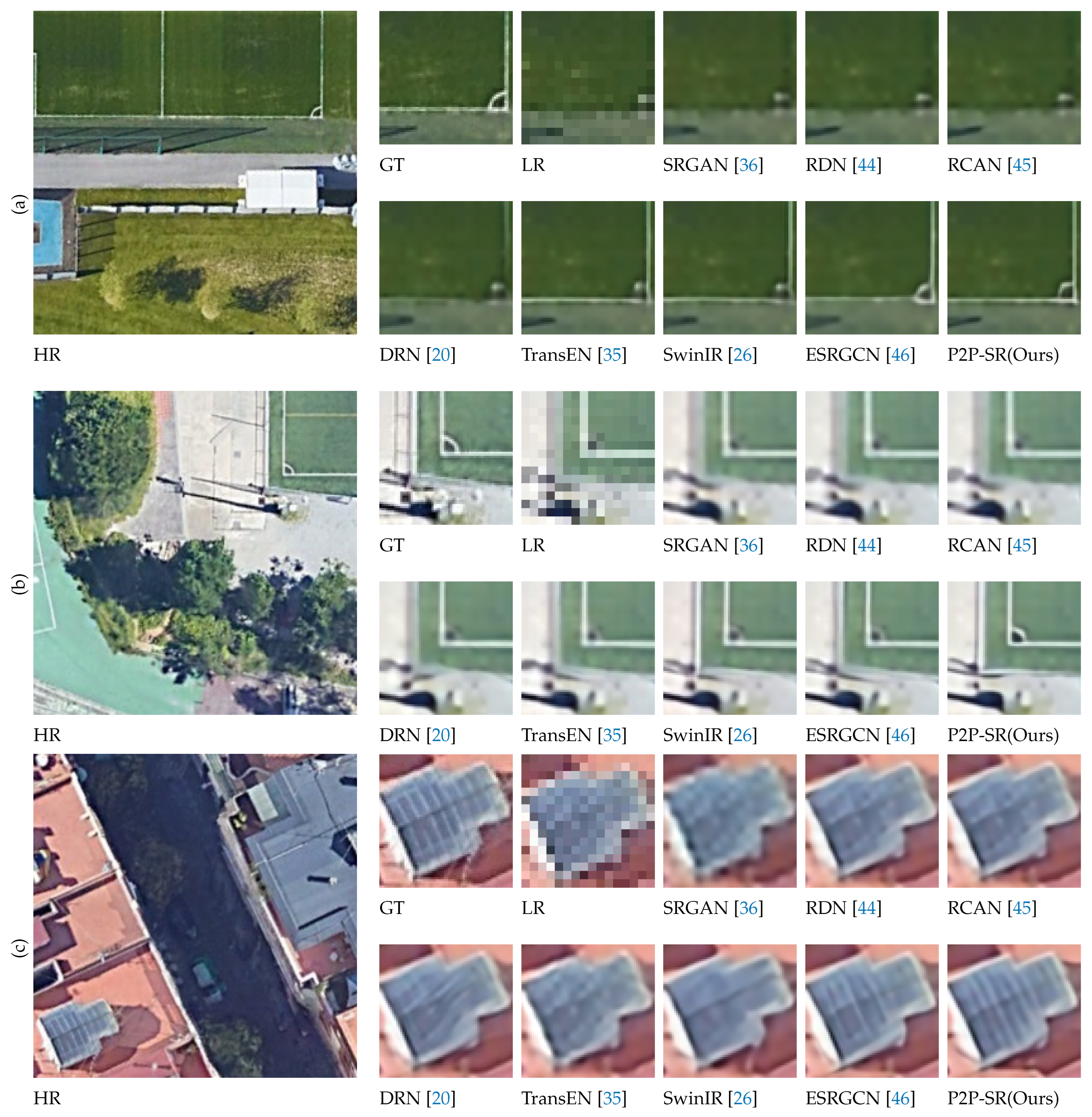
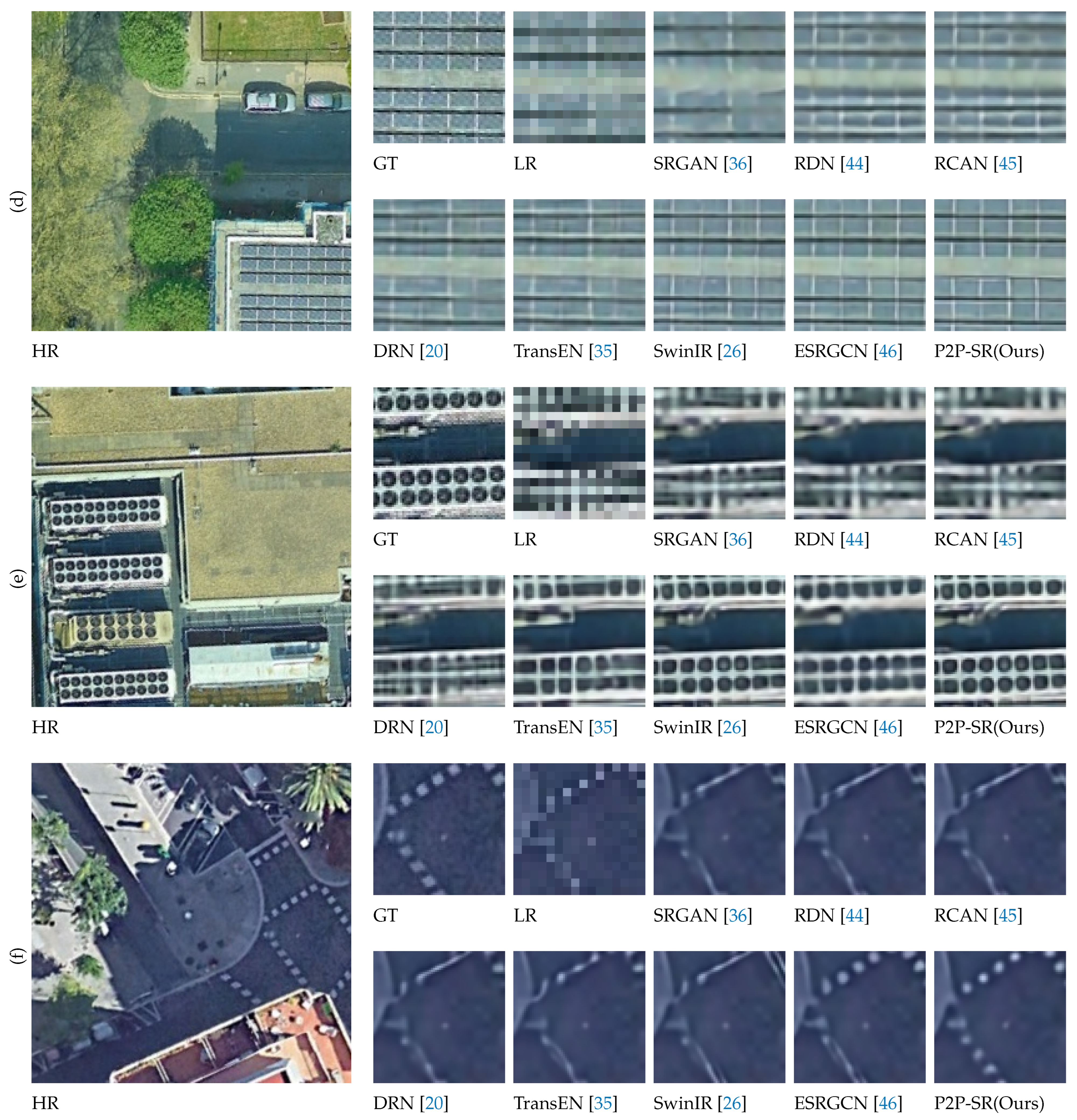
The visual comparison of the output of each method is shown in Figure 2. From the visual comparison, our method has the advantage in reducing both the loss of details and the appearance of pseudo-detail during super resolution. Both PSNR and the structure similarity index measure (SSIM) were used as network performance evaluation metrics. The comparison of each network performance is shown in Table 1. Except for one value, our method outperformed existing SOTA methods. In the two-times super-resolution task, our method achieved a PSNR improvement of 0.29∼2.48 dB over the existing optimal method. In the four-times super-resolution task, our method achieved a PSNR improvement of 0.47∼3.57 dB over the existing optimal method. It can be seen that our method has a more significant performance improvement on the four-times super-resolution task than on the two-times task. This is because the ill-posedness of four-times super resolution is more severe than two times. The four-times super resolution has a more urgent need for additional supervision to reduce the ill-posedness. Accordingly, greater gains can be obtained by using a multi-level supervision structure on four-times super-resolution tasks. This also suggests that the larger the super-resolution scale factor, the greater the multi-level supervision structure needed to introduce adequate supervision. Exploring the benefits of multi-level supervision structures in super-resolution tasks with larger scale factors could be an interesting direction for future research. To validate the statistical significance of the experiments, Friedman’s test, a non-parametric statistical method, was employed to compare various methods. The p-values for PSNR and SSIM were calculated separately. The p-value for PSNR is , and the p-value for SSIM is . These p-values are both lower than the standard threshold of 0.05, indicating significant differences among the compared methods.
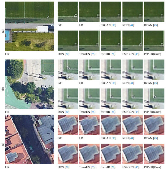

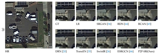
Figure 2.
Comparison of the 4-times super-resolution outputs of P2P-SR and other methods [20,26,35,36,44,45,46]. There are seven sets of images from different scenes. In each set of results, HR is the high-resolution original image, GT is a local zoom of the HR image, and LR is a local zoom of the low-resolution input image. Also shown in each set of pictures are the results of the seven compared methods (a–g) as well as our method.

Table 1.
Performance comparison of different super-resolution methods on three datasets.
Although a two-level supervised network was used, which may bring an increase in parameters, it can be seen that the proposed network still has advantages in terms of parameter quantity and will not bring additional burden to practical applications. As shown in Table 2, the computational complexity of different methods were calculated under our datasets. It can be seen that the proposed method has certain advantages in computational complexity comparing with other comparative methods. As mentioned before, multi-level supervised networks may increase computational complexity for the purpose of improving the performance of super resolution. But it has been proven that the computational complexity of the proposed network has not become a significant drawback of the network.
Table 2.
Comparison of the complexity of the different reconstructed networks under our datasets.
4.3. Ablation Study
Three ablation studies were carried out for the multi-level supervision network structure of our method, the method of dividing the super-resolution scale factor, and the cross-level loss function.
4.3.1. Multi-Level Supervision
To verify the effectiveness of the progressive super-resolution and multi-level supervision network structure of our method, the super-resolution output results for different levels were compared. First, the number of components in our method’s network was reduced to one, setting the super-resolution scale factor of the component to four. The classical one-step super-resolution method was conducted on our network. Second, the number of components in our network was increased to two, setting the super-resolution multiplier to two for both. Third, the number of components in our network was increased to three, setting the super-resolution multiplier to two for both. Third, the number of components in our network was increased to three and the super-resolution scale factor of each component was set to , and two. Finally, the number of components was increased to four and the super-resolution scale factor for each component was set to . In the process of increasing the number of components, supervision was applied at the output of each component.
The experimental results corresponding to different numbers of components are shown in Table 3. As the number of components in the network increased, the PSNR and SSIM of the super-resolution results improved. This indicated that as the number of components in the network increased, the number of supervision levels increased and more supervision images were introduced into the network training process. The network training received more constraints, and the ill-posedness of the super resolution was reduced. This benefited the reconstruction accuracy of the super-resolution results.
Table 3.
Ablation study for different number of super-resolution components.
4.3.2. Scale Factor of Each Component
After increasing the number of components in the network to four, it is worth exploring how to determine the scale factor for each component. In order to verify the effect of different combinations of scale factors of components on the super-resolution results, various combinations were trained and compared. As shown in Table 4, the scale factors were unevenly distributed for the first two combinations and evenly distributed for the last two. The case of uneven distribution of scale factors was divided into a dense distribution in the front section and a dense distribution in the back section. For the case of a dense distribution of the scale factor in the front section, the image output multipliers for each component were 1.3, 1.6, 2 and 4, respectively. For the case of a dense distribution in the latter part of the scale factor, the image output multipliers for the each components were 2, 2.3, 2.6 and 4, respectively. The case of even distribution of scale factors was also divided into equivariate and isometric distributions. For an even distribution of scale factors, the magnification of the output image for each component was set to 1.5, 2, 2.5, 4 and , 2, 2, 4.
Table 4.
Ablation study for different scale factors of super-resolution components.
The experimental results corresponding to the different scale factor distributions are shown in Table 4. The experimental results illustrated that the uneven scale factor distribution had a limited degree of enhancement on the super-resolution result. A multi-level supervision structure with evenly distributed scale factors was effective in improving super-resolution results, and the best super-resolution results were obtained when the scale factors were distributed in an equiproportional series.
4.3.3. Loss Function
In order to fully exploit the effect of the multi-level supervision structure, the cross-level loss function was designed. To verify the usefulness of the cross-level loss function, ablation studies were conducted for different combinations of loss functions. As shown in Table 5, four combinations of loss functions were compared. In the first three combinations of loss functions, the same loss function is applied at the output of each BSRC. In the first two combinations of loss functions, the same loss function was applied at the output of each BSRC. The loss function for each BSRC was the L1 loss or perceptual loss. In the third combination of loss functions, both L1 loss and perceptual loss were used. The loss function for the first two BSRCs was perceptual loss, and the loss function for the last two BSRCs was L1 loss. The fourth combination of loss functions was the cross-level loss. From the experimental results in Table 5, it can be seen that the loss functions using all L1 loss and all perceptual loss had better performance on PSNR and SSIM respectively. Using both L1 loss and perceptual loss could result in better performance on both PSNR and SSIM. The cross-level loss function further improved the super-resolution performance of the network and achieved the best results.
Table 5.
Ablation study for different loss functions.
5. Conclusions
Super resolution is a typical non-adaptive problem, and the space of all possible functions for mapping from a low-resolution image to a high-resolution image is large. This leads to a loss of detail and pseudo-detail in the super-resolution output. Increasing the number of supervisions in the super-resolution process can effectively reduce the ill-posedness. Therefore, a progressive super-resolution network based on multi-level supervision was proposed, and a lightweight BSRC with adjustable scale factor was designed. The relationship between the number of BSRCs, the scale factor of each BSRC, and the performance of the multi-level supervision network was explored. Additionally, a cross-level loss function suitable for the multi-level supervision structure was designed. To fully test the performance of the super-resolution network, a dataset containing various types of ground regions was produced. Experiments were conducted on two publicly available datasets and the new dataset. The experimental results showed that the P2P-SR network outperformed existing SOTA methods. By further analyzing the experimental results, it was found that multi-level supervision has greater performance gains in super-resolution tasks with larger scale factors. It is speculated that the multi-level supervision network will have better performance in super-resolution tasks above four times. In future research, experiments will be conducted with multi-level supervision networks in super-resolution tasks at larger magnifications such as five times, eight times, and so on.
Also, the relationship between multi-level supervision and the reduction in super-resolution ill-posedness will be further explored.
Author Contributions
Conceptualization, Q.X. and J.G.; data curation, M.L. and Q.Z.; methodology, Q.X. and M.L.; supervision, J.G. and Q.X.; validation, M.L.; writing—original draft, M.L.; writing—review and editing, M.L. and Q.Z. All authors have read and agreed to the published version of the manuscript.
Funding
This work was supported by the National Natural Science Foundation of China under Grant 61972021.
Institutional Review Board Statement
Not applicable.
Informed Consent Statement
Not applicable.
Data Availability Statement
The data presented in this study are available on request from the corresponding author. The data are not publicly available due to confidentiality.
Conflicts of Interest
The authors declare no conflict of interest.
References
- Jin, Y.; Zhang, Y.; Cen, Y.; Li, Y.; Mladenovic, V.; Voronin, V. Pedestrian detection with super-resolution reconstruction for low-quality image. Pattern Recognit. 2021, 115, 107846. [Google Scholar] [CrossRef]
- Wang, L.; Li, D.; Zhu, Y.; Tian, L.; Shan, Y. Dual super-resolution learning for semantic segmentation. In Proceedings of the IEEE/CVF Conference on Computer Vision and Pattern Recognition, Seattle, WA, USA, 13–19 June 2020; pp. 3774–3783. [Google Scholar]
- Ibragimov, B.; Prince, J.L.; Murano, E.Z.; Woo, J.; Stone, M.; Likar, B.; Pernuš, F.; Vrtovec, T. Segmentation of tongue muscles from super-resolution magnetic resonance images. Med. Image Anal. 2015, 20, 198–207. [Google Scholar] [CrossRef] [PubMed]
- Shermeyer, J.; Van Etten, A. The Effects of Super-Resolution on Object Detection Performance in Satellite Imagery. In Proceedings of the IEEE/CVF Conference on Computer Vision and Pattern Recognition (CVPR) Workshops, Long Beach, CA, USA, 15–20 June 2019. [Google Scholar]
- Zou, Z.; Shi, Z. Ship detection in spaceborne optical image with SVD networks. IEEE Trans. Geosci. Remote Sens. 2016, 54, 5832–5845. [Google Scholar] [CrossRef]
- Chen, Y.; Liu, S.; Wang, X. Learning continuous image representation with local implicit image function. In Proceedings of the IEEE/CVF Conference on Computer Vision and Pattern Recognition, Nashville, TN, USA, 20–25 June 2021; pp. 8628–8638. [Google Scholar]
- Lei, S.; Shi, Z.; Wu, X.; Pan, B.; Xu, X.; Hao, H. Simultaneous super-resolution and segmentation for remote sensing images. In Proceedings of the IGARSS 2019—2019 IEEE International Geoscience and Remote Sensing Symposium, Yokohama, Japan, 28 July–2 August 2019; pp. 3121–3124. [Google Scholar]
- Wang, Y.; Bashir, S.M.A.; Khan, M.; Ullah, Q.; Wang, R.; Song, Y.; Guo, Z.; Niu, Y. Remote sensing image super-resolution and object detection: Benchmark and state of the art. Expert Syst. Appl. 2022, 197, 116793. [Google Scholar] [CrossRef]
- Rogan, J.; Chen, D. Remote sensing technology for mapping and monitoring land-cover and land-use change. Prog. Plan. 2004, 61, 301–325. [Google Scholar] [CrossRef]
- Li, J.; Pei, Y.; Zhao, S.; Xiao, R.; Sang, X.; Zhang, C. A review of remote sensing for environmental monitoring in China. Remote Sens. 2020, 12, 1130. [Google Scholar] [CrossRef]
- Joyce, K.E.; Belliss, S.E.; Samsonov, S.V.; McNeill, S.J.; Glassey, P.J. A review of the status of satellite remote sensing and image processing techniques for mapping natural hazards and disasters. Prog. Phys. Geogr. 2009, 33, 183–207. [Google Scholar] [CrossRef]
- Anwar, S.; Khan, S.; Barnes, N. A deep journey into super-resolution: A survey. ACM Comput. Surv. (CSUR) 2020, 53, 1–34. [Google Scholar] [CrossRef]
- Wang, Z.; Chen, J.; Hoi, S.C. Deep learning for image super-resolution: A survey. IEEE Trans. Pattern Anal. Mach. Intell. 2020, 43, 3365–3387. [Google Scholar] [CrossRef]
- Chen, H.; He, X.; Qing, L.; Wu, Y.; Ren, C.; Sheriff, R.E.; Zhu, C. Real-world single image super-resolution: A brief review. Inf. Fusion 2022, 79, 124–145. [Google Scholar] [CrossRef]
- Fernandez-Beltran, R.; Latorre-Carmona, P.; Pla, F. Single-frame super-resolution in remote sensing: A practical overview. Int. J. Remote Sens. 2017, 38, 314–354. [Google Scholar] [CrossRef]
- Wang, P.; Bayram, B.; Sertel, E. A comprehensive review on deep learning based remote sensing image super-resolution methods. Earth-Sci. Rev. 2022, 232, 104110. [Google Scholar] [CrossRef]
- Kim, J.; Lee, J.K.; Lee, K.M. Accurate image super-resolution using very deep convolutional networks. In Proceedings of the IEEE Conference on Computer Vision and Pattern Recognition, Las Vegas, NV, USA, 26 June–1 July 2016; pp. 1646–1654. [Google Scholar]
- Lugmayr, A.; Danelljan, M.; Van Gool, L.; Timofte, R. Srflow: Learning the super-resolution space with normalizing flow. In Proceedings of the Computer Vision–ECCV 2020: 16th European Conference, Glasgow, UK, 23–28 August 2020,; Proceedings, Part V 16; Springer: Berlin, Germany, 2020; pp. 715–732. [Google Scholar]
- Kim, Y.; Son, D. Noise conditional flow model for learning the super-resolution space. In Proceedings of the IEEE/CVF Conference on Computer Vision and Pattern Recognition, Nashville, TN, USA, 20–25 June 2021; pp. 424–432. [Google Scholar]
- Guo, Y.; Chen, J.; Wang, J.; Chen, Q.; Cao, J.; Deng, Z.; Xu, Y.; Tan, M. Closed-loop matters: Dual regression networks for single image super-resolution. In Proceedings of the IEEE/CVF Conference on Computer Vision and Pattern Recognition, Seattle, WA, USA, 13–19 June 2020; pp. 5407–5416. [Google Scholar]
- Dong, C.; Loy, C.C.; He, K.; Tang, X. Learning a deep convolutional network for image super-resolution. In Proceedings of the European Conference on Computer Vision, Zurich, Switzerland, 6–12 September 2014; Proceedings, Part IV 13; Springer: Berlin, Germany, 2014; pp. 184–199. [Google Scholar]
- Mao, X.J.; Shen, C.; Yang, Y.B. Image restoration using convolutional auto-encoders with symmetric skip connections. arXiv 2016, arXiv:1606.08921. [Google Scholar]
- Shi, W.; Caballero, J.; Huszár, F.; Totz, J.; Aitken, A.P.; Bishop, R.; Rueckert, D.; Wang, Z. Real-time single image and video super-resolution using an efficient sub-pixel convolutional neural network. In Proceedings of the IEEE Conference on Computer Vision and Pattern Recognition, Las Vegas, NV, USA, 26 June–1 July 2016; pp. 1874–1883. [Google Scholar]
- Dong, C.; Loy, C.C.; Tang, X. Accelerating the super-resolution convolutional neural network. In Proceedings of the European Conference on Computer Vision–ECCV 2016: 14th European Conference, Amsterdam, The Netherlands, 11–14 October 2016; Proceedings, Part II 14; Springer: Berlin, Germany, 2016; pp. 391–407. [Google Scholar]
- Chen, H.; Wang, Y.; Guo, T.; Xu, C.; Deng, Y.; Liu, Z.; Ma, S.; Xu, C.; Xu, C.; Gao, W. Pre-Trained Image Processing Transformer. In Proceedings of the IEEE/CVF Conference on Computer Vision and Pattern Recognition (CVPR), Nashville, TN, USA, 20–25 June 2021; pp. 12299–12310. [Google Scholar]
- Liang, J.; Cao, J.; Sun, G.; Zhang, K.; Van Gool, L.; Timofte, R. SwinIR: Image Restoration Using Swin Transformer. In Proceedings of the IEEE/CVF International Conference on Computer Vision (ICCV) Workshops, Montreal, BC, Canada, 11–17 October 2021; pp. 1833–1844. [Google Scholar]
- Lu, Z.; Li, J.; Liu, H.; Huang, C.; Zhang, L.; Zeng, T. Transformer for Single Image Super-Resolution. In Proceedings of the IEEE/CVF Conference on Computer Vision and Pattern Recognition (CVPR) Workshops, New Orleans, LA, USA, 18–24 June 2022; pp. 457–466. [Google Scholar]
- Liebel, L.; Körner, M. Single-image super resolution for multispectral remote sensing data using convolutional neural networks. ISPRS-Int. Arch. Photogramm. Remote Sens. Spat. Inf. Sci. 2016, 41, 883–890. [Google Scholar] [CrossRef]
- Tuna, C.; Unal, G.; Sertel, E. Single-frame super resolution of remote-sensing images by convolutional neural networks. Int. J. Remote Sens. 2018, 39, 2463–2479. [Google Scholar] [CrossRef]
- Lei, S.; Shi, Z.; Zou, Z. Super-resolution for remote sensing images via local–global combined network. IEEE Geosci. Remote. Sens. Lett. 2017, 14, 1243–1247. [Google Scholar] [CrossRef]
- Jiang, K.; Wang, Z.; Yi, P.; Jiang, J.; Xiao, J.; Yao, Y. Deep distillation recursive network for remote sensing imagery super-resolution. Remote Sens. 2018, 10, 1700. [Google Scholar] [CrossRef]
- Hu, J.F.; Huang, T.Z.; Deng, L.J.; Dou, H.X.; Hong, D.; Vivone, G. Fusformer: A transformer-based fusion network for hyperspectral image super-resolution. IEEE Geosci. Remote Sens. Lett. 2022, 19, 1–5. [Google Scholar] [CrossRef]
- Tu, J.; Mei, G.; Ma, Z.; Piccialli, F. SWCGAN: Generative adversarial network combining swin transformer and CNN for remote sensing image super-resolution. IEEE J. Sel. Top. Appl. Earth Obs. Remote Sens. 2022, 15, 5662–5673. [Google Scholar] [CrossRef]
- An, T.; Zhang, X.; Huo, C.; Xue, B.; Wang, L.; Pan, C. TR-MISR: Multiimage super-resolution based on feature fusion with transformers. IEEE J. Sel. Top. Appl. Earth Obs. Remote Sens. 2022, 15, 1373–1388. [Google Scholar] [CrossRef]
- Lei, S.; Shi, Z.; Mo, W. Transformer-Based Multistage Enhancement for Remote Sensing Image Super-Resolution. IEEE Trans. Geosci. Remote. Sens. 2021, 60, 5615611. [Google Scholar] [CrossRef]
- Ledig, C.; Theis, L.; Huszár, F.; Caballero, J.; Cunningham, A.; Acosta, A.; Aitken, A.; Tejani, A.; Totz, J.; Wang, Z.; et al. Photo-realistic single image super-resolution using a generative adversarial network. In Proceedings of the IEEE Conference on Computer Vision and Pattern Recognition, Honolulu, HI, USA, 21–26 July 2017; pp. 4681–4690. [Google Scholar]
- Ahn, N.; Kang, B.; Sohn, K.A. Image super-resolution via progressive cascading residual network. In Proceedings of the IEEE Conference on Computer Vision and Pattern Recognition Workshops, Salt Lake City, UT, USA, 18–23 June 2018; pp. 791–799. [Google Scholar]
- Nathan, S.; Kansal, P. Leveraging multi scale backbone with multilevel supervision for thermal image super resolution. In Proceedings of the IEEE/CVF Conference on Computer Vision and Pattern Recognition, Nashville, TN, USA, 20–25 June 2021; pp. 4332–4338. [Google Scholar]
- Johnson, J.; Alahi, A.; Fei-Fei, L. Perceptual losses for real-time style transfer and super-resolution. In Proceedings of the European Conference on Computer Vision–ECCV 2016: 14th European Conference, Amsterdam, The Netherlands, 11–14 October 2016; Proceedings, Part II 14; Springer: Berlin, Germnay, 2016; pp. 694–711. [Google Scholar]
- Tang, Z.; Luo, L.; Xie, B.; Zhu, Y.; Zhao, R.; Bi, L.; Lu, C. Automatic sparse connectivity learning for neural networks. IEEE Trans. Neural Netw. Learn. Syst. 2022, 34, 7350–7364. [Google Scholar] [CrossRef] [PubMed]
- Huang, Q. Weight-quantized squeezenet for resource-constrained robot vacuums for indoor obstacle classification. AI 2022, 3, 180–193. [Google Scholar] [CrossRef]
- Hu, W.; Che, Z.; Liu, N.; Li, M.; Tang, J.; Zhang, C.; Wang, J. Channel Pruning via Class-Aware Trace Ratio Optimization. IEEE Trans. Neural Netw. Learn. Syst. 2023. [Google Scholar] [CrossRef] [PubMed]
- Hsia, C.H.; Lee, Y.H.; Lai, C.F. An Explainable and Lightweight Deep Convolutional Neural Network for Quality Detection of Green Coffee Beans. Appl. Sci. 2022, 12, 10966. [Google Scholar] [CrossRef]
- Zhang, R.; Isola, P.; Efros, A.A.; Shechtman, E.; Wang, O. The unreasonable effectiveness of deep features as a perceptual metric. In Proceedings of the IEEE Conference on Computer Vision and Pattern Recognition, Salt Lake City, UT, USA, 18–23 June 2018; pp. 586–595. [Google Scholar]
- Zhang, Y.; Li, K.; Li, K.; Wang, L.; Zhong, B.; Fu, Y. Image super-resolution using very deep residual channel attention networks. In Proceedings of the European Conference on Computer Vision (ECCV), Munich, Germany, 8–14 September 2018; pp. 286–301. [Google Scholar]
- Tian, C.; Yuan, Y.; Zhang, S.; Lin, C.W.; Zuo, W.; Zhang, D. Image super-resolution with an enhanced group convolutional neural network. Neural Netw. 2022, 153, 373–385. [Google Scholar] [CrossRef] [PubMed]
- Yang, Y.; Newsam, S. Bag-of-visual-words and spatial extensions for land-use classification. In Proceedings of the 18th SIGSPATIAL International Conference on Advances in Geographic Information Systems, San Jose, CA, USA, 2–5 November 2010; pp. 270–279. [Google Scholar]
- Xia, G.S.; Hu, J.; Hu, F.; Shi, B.; Bai, X.; Zhong, Y.; Zhang, L.; Lu, X. AID: A benchmark data set for performance evaluation of aerial scene classification. IEEE Trans. Geosci. Remote Sens. 2017, 55, 3965–3981. [Google Scholar] [CrossRef]

Disclaimer/Publisher’s Note: The statements, opinions and data contained in all publications are solely those of the individual author(s) and contributor(s) and not of MDPI and/or the editor(s). MDPI and/or the editor(s) disclaim responsibility for any injury to people or property resulting from any ideas, methods, instructions or products referred to in the content. |
© 2023 by the authors. Licensee MDPI, Basel, Switzerland. This article is an open access article distributed under the terms and conditions of the Creative Commons Attribution (CC BY) license (https://creativecommons.org/licenses/by/4.0/).