Application of Compound Terrain Factor LSW in Vegetation Cover Evaluation

Abstract

Aiming at the limited degree of revealing vegetation growth pattern by simple topographic factors, it is essential to find an index that can explain the vegetation cover mechanism to a greater extent. By introducing a certainty factor into vegetation cover evaluation, LSW, LS, topographic wetness index, and aspect were also chosen to carry out control group experiments. The grid digital elevation model of 10 disaster-stricken counties (cities) in Sichuan Province was used as the basis to obtain LSW, while vegetation susceptibility levels were categorized using the natural breaks classification. The results of the multi-factor analysis demonstrated that the certainty factor corresponding to LSW climbed linearly from negative to positive values as the susceptibility level rose, indicating that it was highly correlated with vegetation cover and had an obvious advantage in revealing the vegetation growth potential. Statistically, the vegetation occurrence rate increased regularly with the improvement of the susceptibility level, in which the high and very high susceptibility zones corresponded to 83.66% and 89.95% of vegetation coverage respectively, suggesting a good consistency between the delineated high susceptibility areas and the actual vegetation cover. The findings proved that LSW has a substantial advantage in evaluating vegetation cover, with an evaluation model accuracy of 72.9%. It has been established that LSW will serve as a promising new model for assessing vegetation restoration and planning.

1. Introduction

With the issuance and implementation of several international environmental conventions, such as the Convention on Biological Diversity (https://www.cbd.int, accessed on 15 May 2023) and the Convention on International Trade in Endangered Species of Wild Fauna and Flora (https://cites.org/eng, accessed on 15 May 2023), awareness of environmental protection continues to grow. Land cover type is closely linked to ecological development [1]. As an important component of land cover, vegetation has been given high priority. By evaluating the extent of vegetation cover in the study area, the regional conditions of biological resources can be objectively reflected and play an indicative role in describing the severity of soil erosion [2].

The existing vegetation cover evaluation methods rely on single or several types of vegetation index analysis implementation, whose principle is to combine the spectral information in remote sensing images to mine a specific vegetation cover or soil reflectance [3]. Currently, the dominant vegetation indices include the Normalized Difference Vegetation Index (NDVI) and the Ratio Vegetation Index (RVI), et al. However, these factors have inherent shortcomings. For example, the NDVI is susceptible to saturation on moderate to high surface biomass conditions [4], and the RVI is significantly less sensitive when applied to areas with low vegetation cover. The positional relationship between the sensor and the vegetation, such as the vegetation coverage obtained by observing from the tree tops (where the observed object is located at the substellar point), the light-facing side (forward scattering), and the back-lighting side (back scattering), etc., will make a difference [5,6], which results in unavoidable errors in the vegetation cover assessment. Moreover, the obtained vegetation indices can be biased due to atmospheric scattering and absorption, soil background, and angular variations [6,7]. It is important to note that vegetation indices have limitations when used for assessing vegetation growth potential, even though they are widely used for vegetation cover evaluation. Correa-Díaz et al. [8] found that an increase in forest canopy NDVI did not correlate with tree growth trends when used to assess long-term trends in greenness and land surface phenology. Coulthard et al. [9] pointed out that the correspondence between vegetation index and vegetation biomass will be ambiguous for high-altitude forested areas and low-elevation areas with greater species richness (covering trees, shrubs, grasslands, etc.). Existing vegetation indices determine whether vegetation is covered or not only by the magnitude of their values, ignoring the influence of the site environment on the growth potential of vegetation, and failing to reveal the mechanism of vegetation within the slope. Therefore, it is urgent to seek a new vegetation appraisal method.

Topography is the carrying container of ecosystems, and topographic factors are gradually gaining attention in resource and environmental planning and management as a sort of intuitive representation [10,11]. In recent years, many scholars have started to explore the interconnection between topography and vegetation cover, and have conducted studies with different emphases based on their respective fields of application. Some scholars used multi-temporal remote sensing images and digital elevation model (DEM) as data sources, along with trend analysis, factor detection, and interaction detection methods to try to decipher the extent to which human activities have driven vegetation changes, taking river valleys and river headwater regions as objects [12,13]. Through geographically weighted regression, multiple regression, and threshold regression, some researchers have revealed the multi-scale spatial relationships between topographic attributes and vegetation cover [14,15]. These findings provide a scientific basis for ecological environmental protection and assessment. Furthermore, some scholars have considered vegetation and topography as key elements in evaluating ecosystem services, and have also conducted topographic correlations for ecosystems with different vegetation types to offer theoretical guidance and decisions for sustainable development in high plateaus and mountainous areas [16,17]. However, the studies of the relevance between vegetation cover and topography are confined to the traditional simple topographic factors such as slope and elevation, which cannot reveal the hidden laws in depth due to the limitations of these factors. Besides, some scholars have taken erosion control as an entry point to differentiate how various environmental factors, such as climate, topography, vegetation, and human activities, contribute to erosion changes [18,19], while seasonal variations are taken into account. Additionally, some scholars developed the SLTNI (local window terrain niche index based on similar habitat) and compared it to the traditional TNI (terrain niche index) and LTNI (local window terrain niche index) to demonstrate its superiority in assessing vegetation cover [20]. Nevertheless, the slope body exists as an independent natural topographic entity, but few scholars have explored the linkages between slope development, soil erosion and vegetation growth from an integrated perspective [21,22]. Taking the morphological characteristics of the slope surface as the basis, scholars have respectively explored the influence of slope length (L) and slope width factor (W) on soil erosion [23,24], as well as investigated the influence of the slope factor (S) on the sediment-discharge relationship [25,26]. These studies present valuable decision-making knowledge to serve for gully erosion control, and they also provide ideas for finding novel methods of assessing vegetation growth potential. Synthesizing existing studies related to topography and vegetation growth, we infer that there is an important association between slope conditions and vegetation development. As a comprehensive slope indicator that balances the contribution of each factor, LSW (Length, Slope and Width Factor) is the potential factor to fill this gap, so exploring the relationship between LSW and vegetation growth potential becomes the key point of this paper.

The above analysis suggests that topographic factors and vegetation indices complement each other and provide a key basis for land cover classification [27]. This study intends to elucidate the vegetation cover mechanism from the perspective of digital terrain analysis (DTA) with the following objectives: (1) to take vegetation cover evaluation as a starting point and fill in the local one-sidedness of image spectral information from the perspective of data sources; (2) to explain the association between the novel factor LSW and soil erosion in qualitative and quantitative terms; (3) to investigate the suitability of the bivariate model (certainty factor, CF) applied to the assessment of vegetation growth and development, and to make directional attempts for the application of the LSW.

2. Mechanisms of LSW Factors on Vegetation Cover

2.1. Response of LSW Factors to Hydrologic Conditions

The current slope and length factor (LS) can describe the shape of the slope’s vertical profile and are important indicators of hydrological connectivity and soil erosion. However, the multiplicative fusion method has a tendency to compress information related to topographic features [28,29], which can lead to distorted representations. In contrast, the LSW factor originated from LS, while creatively integrating LS with the slope width (W) factor in the field of engineering applications. Due to the late introduction of LSW, the application field of this factor needs to be further explored. Theoretically, the slope width integrally represents the hydrodynamic law of the slope: the larger the slope width, the stronger the confluence capacity of the slope where the grid cell lies compared to other slopes [30,31]. Based on the transverse profile analysis, the slope section’s ductility range expands with increasing slope width, which is compatible with the water convergence conditions. According to Li et al. [32], the horizontal movement of the water flow is mostly influenced by the matrix potential gradient and gravitational potential gradient in the soil. Its horizontal motion is also more apparent when the slope is well ductile. Considering that slope width can more accurately express hydrological connectivity, regions with large slope width suggest that there is abundant surface water flow, which controls solute exchange and streambed sediment interactions [33], ensuring high permeability sediment thickness in the area. This creates a beneficial cycle for hydraulic exchange and eventually encourages the growth and development of nearby plants.

2.2. Geometric Description of the Gully by LSW and Corresponding Ecological Response

First, existing research indicates that slope width and gully extensibility are negatively correlated [24]. The term “extensibility” refers to the ratio of the length to width of the gully’s outer rectangle perpendicular to the slope surface. As a result, the larger the slope width within the slope, the more elongated the internal gullies are. Since the cross-sectional morphology of fine gullies is insensitive to changes in slope length [34], and such structures do not contribute significantly to lateral erosion of the valley, the low rate of gully wall expansion can preserve the current basic morphology of the river valley [35]. In addition, elongated gullies have a positive impact on increasing surface area and raising ground temperature, and play a similar role to trenching in cultivated areas to achieve water conservation and retention [36], thereby improving soil water and salt distribution and soil quality status [37]. Furthermore, it has been observed that there is an inverse correlation between the slope width and the variability of the gully slope [24]. Gully slope variability is defined as the ratio of the elevation difference between the head and tail of the gully to its length. For regions with wider slopes, the gravitational potential energy in the descending direction of the slope does not change greatly. As a result, the erosion effect of surface runoff is not significant, and the relatively slow water flow rate provides a greater opportunity for organic deposition [38,39], again creating possible conditions for vegetation growth.

Based on the close dependence of the LS factor on soil loss and erosion, it is initially assumed that the LSW has a certain influence on the growth of greenery, and the LSW factor of the study area is calculated with reference to the method of G_L + G_S + G_W (where G_L, G_S and G_W are the normalized values of L, S and W, respectively), with a hope to find new applications of the new factor on vegetation cover evaluation.

3. Materials and Methods

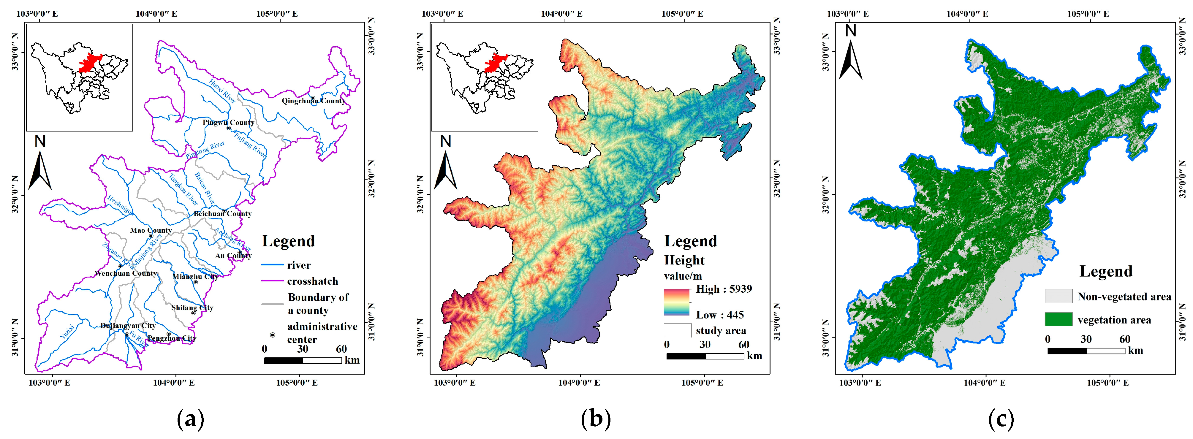
3.1. Overview of the Study Area

In this paper, a total of 10 counties (cities) including Wenchuan, Beichuan, Mianzhu, Shifang, Qingchuan, Mao, An, Dujiangyan, Pingwu, and Pengzhou were selected as the study area [40]. The study area is depicted in Figure 1a, with a land size of 26,177 km².

The DEM used herein are ASTER GDEM v3 data collaboratively developed by METI (Ministry of Economy, Trade and Industry) of Japan and NASA (National Aeronautics and Space Administration) of the United States, and jointly distributed to the public freely [41] (Data webpage: https://urs.earthdata.nasa.gov/, accessed on 5 April 2023). After acquiring the data, the DEM of the target study area was obtained by stitching, projecting the coordinate system, specifying the extent of cropping, and filling the pits in ArcGIS 10.7 for the subsequent extraction of the derived topographic factors. Considering that the DEM dataset did not have significant discontinuities or large deviations, the average value stitching approach was chosen. The projection coordinate system was set to WGS_1984_UTM_Zone_47N. Additionally, the vector data of 10 counties (cities) in the hardest-hit areas were obtained from the National Geomatics Center of China (data webpage: http://www.ngcc.cn/ngcc/, accessed on 7 April 2023).

3.1.1. Terrain Topography

The southeastern part of the 10 disaster-hit counties (cities) is adjacent to the Chengdu Plain, which is known as the “heavenly country”, and has a flat topography with little undulation, making it an important crop-growing area in China since ancient times. The western part of the study area has peaks such as Mount Siguniang and Xuelongbao, so it can be found in conjunction with Figure 1b that the overall topography of the 10 hardest-hit counties (cities) is high in the west and low in the east. The central part of the study area is the Longshan Mountain Range, which is relatively high in elevation, while the western part of the area gradually rises in relief and transitions to the Tibetan Plateau.

3.1.2. Meteorology and Hydrology

In view of the close proximity of this test area to the Qinling Mountains–Huaihe River Line in China, the region is controlled by tropical maritime air masses and polar continental air masses alternately throughout the year, and a subtropical monsoon climate prevails in the 10 counties (cities), except for Mao County and Wenchuan County. Mao County is situated in the western part of the study area, with a predominantly highland monsoon climate. The average elevation of the county can reach 3000 m, with low temperature and lack of precipitation all year round. Wenchuan County has a temperate monsoon climate with hot and rainy summers, cold and dry winters, and significant monsoon influence. In fact, due to the wide disparity in elevation between the southeastern and northwestern parts of the county, its vertical climate zones also show remarkable variability. The 10 hardest-hit counties are characterized by warm winters and cool summers, huge temperature differences between day and night, dry and windy climate, and dry-hot valley. The main rivers in the study area are the main stream of the Minjiang River, the Zagunao River, the Mianyuan River, and the Jianjiang River.

3.1.3. Vegetation Cover

In conjunction with the climatic characteristics of the vast majority of counties (cities) in the study area, the annual summer could usher in the same period of rain and heat. As verified by the Sichuan Statistical Yearbook 2017 (data webpage: http://tjj.sc.gov.cn/scstjj/c105855/nj.shtml, accessed on 13 May 2013), the average precipitation in a single month during the summer period will be 180 mm, 2~3 times more than in other months, with an average temperature of about 25 degrees Celsius. To focus on the influence of topography on plant growth, it is important to eliminate the effect of other factors. Hence, the remote sensing data used in this study are Landsat-8 satellite images taken in May 2017. It is mid to late spring in the northern hemisphere, when the snow and ice cover has largely melted, making it easy to use supervised classification methods to delineate vegetation growth areas. In addition, the temperature and rainfall of May do not reach the optimum stage of vegetation growth, and the topographic effect of the site environment will be more prominent in this stage [42,43], offering a more direct and higher reference value for the field of DTA.

Landsat-8 is equipped with an operational land imager (OLI) sensor that uses a pan-sharpening spectral range to make the contrast between vegetation and non-vegetation on panchromatic images become large. The advanced technical design also eliminates the effect of partial water vapor absorption [44], providing a reliable and stable data source for accurate acquisition of vegetation information. The five images downloaded from the National Geospatial Data Cloud were all shot in 2017 (Data webpage: https://www.gscloud.cn/, accessed on 4 May 2023); one was taken on 26 May, two on 8 May, and the remaining two on 1 May. With ENVI 5.3 software as the platform, the visual interpretation of the acquired remote sensing images was enhanced after a series of operations such as radiometric calibration, atmospheric correction, geometric correction, and edge enhancement. By using the Computer ROI (Region of Interest) Separability tool in ENVI 5.3 software, it was possible to calculate the statistical distances between vegetated and non-vegetated areas (including urban and rural residential, transportation land, construction land, and water). This index measures the separability of the training samples based on the Jeffries–Matusita distance and the transformation separation degree. The value of separability ranges from 0 to 2. It is qualified when the value is greater than 1.8 [45], and the larger the separation degree is, the easier it is to distinguish the two geographical features. Upon calculation, the separability of vegetation from other features was 1.947624, 1.966721, 1.994156, and 1.979636, respectively. Given that the separability of vegetation from other features is greater than 1.9, the operability of supervised classification is illustrated at a theoretical level [45]. Based on existing studies [46,47,48], it is known that Maximum Likelihood is the nonlinear classification method that minimizes the probability of classification error based on the Bayesian criterion. The classifier’s excellent and robust classification has been demonstrated in numerous studies, making it ideal for this study. Meanwhile, a clustering method [49] is applied to smooth the fragmented patches in the classification results, and the smoothed supervised classification results are used as the initial classification data. Sample areas were randomly selected from GF-1 remote sensing imagery to collect the real initial classification of feature types (image download webpage: http://www.sasclouds.com/chinese/normal/, accessed on 6 May 2023), with the number of samples of each type being more than 50. The overall accuracy of 93.85% and the Kappa coefficient of 0.9231 were obtained after performing the classification accuracy evaluation, which provided a reliable guarantee for the follow-up experiments.

Based on the resolution of Landsat-8 data is 30 m × 30 m, fine vegetation type identification is difficult to achieve [50]. Therefore, only vegetation and non-vegetation areas were distinguished in this study, and the final vegetation cover data are obtained, as shown in Figure 1c.

3.2. Database Construction

For a comprehensive assessment of the evaluation method proposed in this paper, it is crucial to construct a diversified and sufficient number of datasets. On account of the existing studies [51], it has been shown that the height of undulation shows a tendency to first increase and then stabilize with the increase of the analysis window. In this paper, combining the Chinese macro-geomorphic classification standard [51,52] with the actual situation of the study area, the optimal analysis window for the undulation height of the study area was determined to be 15 × 15 pixels by using the neighborhood analysis method. The study area can be divided into six topographic categories according to the height of relief, namely plains (relief < 30 m), terraces (30 m < relief < 70 m), hills (70 m < relief < 200 m), small rolling mountains (200 m < relief < 500 m), medium rolling mountains (500 m < relief < 1000 m), and large rolling mountains (relief > 1000 m). After dividing the terrain categories based on the regularized knowledge, each kind of terrain is selected a nine km × 9 km square representative area as the experimental object, and six experimental areas are selected as shown in Figure 2. Among them, test areas 1~6 represent plains, terraces, hills, small rolling hills, medium rolling hills, and large rolling hills, respectively.

3.3. Slope Factor Extraction

By referencing the existing mature algorithms [28,53,54,55], the LSW and LS factors of the test area were obtained. The extraction of slope width first requires obtaining the catchment accumulation based on the depression-free DEM, and the key to sub-basin division lies exactly in the selection of the catchment accumulation threshold, which determines the shape of the river network. In this paper, the second order derivative analysis of river network density is applied to determine the appropriate threshold for flow accumulation [56], and the specific extraction process is as follows:

Using the hydrology tool, a total of 12 catchment accumulation thresholds from 5000 to 60,000 are set at equal intervals of 5000, generating the river network separately. To obtain the function of flow accumulation threshold and river network density, multi-class functions such as logarithmic function and composite function were used to carry out regression fitting. The results showed that the power function had the best fit, and the R2 (coefficient of determination) of the fit was up to 0.9995. The obtained function expression is shown in Equation (1):

$$\mathrm{y}=23{.432\mathrm{x}}^{-0.491}$$

(1)

where y is the density of the river network (km/km²); x is the threshold of catchment accumulation.

The second order derivative of the power function relation yields Equation (2).

$${\mathrm{y}}^{\prime \prime }=17.154{\mathrm{x}}^{-2.491}$$

(2)

The geometric information is calculated and counted, while the accumulation threshold is brought into Equation (2), resulting in the corresponding hydrological information shown in Figure 3.

Analysis of Figure 3 shows that when the river network threshold was raised from the initial value to 25,000, the reduction of river network density was remarkable, followed by a sudden change and a slow flattening trend. The inflection point of the second derivative function of river network density occurs at the river network threshold of 55,000, and the tendency of hydrological characteristic parameters such as river network density remains basically unchanged. Finally, the optimal threshold value of 55,000 was selected to extract the river network. Subsequently, the “Basin”, “Snap Pour Point” and “Watershed” functions were executed in the Hydrology toolbox of ArcGIS 10.7 to divide the sub-watersheds. On this basis, the delineated watershed data were imported into the WEPP (Water Erosion Prediction Project). After adopting the function of “Watershed Delineation Analysis” to determine the two parameters of CSA (critical source area) and MSCL (Minimum Source Channel Length), we simulate the slope flow process to generalize the slope surface. Finally, we visualize the slope width with ArcGIS 10.7 [57].

3.4. Vegetation Cover Evaluation Based on Certainty Factor

3.4.1. Certainty Factor Analysis

The Certainty Factor can be used to analyze the sensitivity of factors affecting the occurrence of an event, and is attributed to a binary statistical analysis method [58,59]. In studies exploring ecological responses due to environmental factors, bivariate and multivariate statistical models such as the information value method have been progressively and widely used by researchers [60,61]. Furthermore, CF has been used by many scholars for environmental risk management owing to its spatial predictive ability and its capability to capture complex nonlinear relationships, and thus improve the accuracy of prediction compared with correlation coefficients [62,63]. When using CF to examine the connection between vegetation cover and topographic conditions, it is important to understand that vegetation cover is the dependent variable (i.e., event) and topographic factors are the independent variable. In summary, CF is effectively applicable for the study and is calculated as follows:

$$\mathrm{CF}=\{\begin{array}{c}\frac{\mathrm{PPa}-\mathrm{PPs}}{\mathrm{PPa}(1-\mathrm{PPs})}if:\mathrm{PPa}\ge \mathrm{PPs}\\ \frac{\mathrm{PPa}-\mathrm{PPs}}{\mathrm{PPs}(1-\mathrm{PPa})}if:\mathrm{PPa}<\mathrm{PPs}\end{array}$$

(3)

where PPa is the conditional probability of the event occurring in Grade A, and PPs is the prior probability of the event occurring in the entire study area. Taking this study as an example, LSW is categorized into multiple categories according to its numerical size, such as Grade A, B, and C. PPa is the ratio of the area of vegetation to the total area in Grade A, while PPs is the ratio of the overall vegetation area to the total area of the study region. Similarly, we can derive corresponding CF values for both Grade B and Grade C.

According to the formula, the range of CF coefficients is [–1, 1], which can be divided into three categories by the size of the CF values: (1) When the CF value is very close to 0, such cases make it difficult to identify whether vegetation cover will occur; (2) When the CF is positive, it means that the certainty of vegetation cover occurrence is high. As CF gets closer to 1, it indicates that this grid cell is more likely to be a susceptible area for vegetation cover; (3) When the CF value takes a negative value, it means that the certainty of vegetation cover occurrence is low. The closer the CF is to −1, the less vegetation cover is likely to occur in this cell.

3.4.2. Control Group Factor Selection

In order to verify the validity of the new slope factor for vegetation cover evaluation, it is informative to introduce other types of topographic factors to perform a controlled trial. The control group factors were selected not only to consider the degree to which they affect vegetation growth, but were also focused on reflecting the topographic conditions. After referring to relevant studies of scholars both domestically and abroad, and fully considering the feasibility of acquisition, data scale and scope of the study area, the potential evaluation factors were finally determined, as follows:

• LS factor

Since the Universal Soil Loss Equation (USLE) was proposed by Wischmeier and Smith [64], the LS factor has been widely used to calculate soil erosion prediction in multiple regions and landscapes around the world, and has gradually led to the derivation of the Modified Universal Soil Loss Equation (MUSLE) [65], the Revised Universal Soil Loss Equation (RUSLE) [66], the Chinese Soil Loss Equation (CSLE) [67], and other serialized models suitable for different geographical environments. In view of the fact that the LS factor represents the combined effect of slope span and steepness [68] and that the LSW factor is an improved optimization based on the LS factor, it is necessary to include the LS factor in the control group.

2.

Topographic wetness index (TWI)

Topography will act profoundly on rainfall redistribution [69], which consequently affects the spatial distribution of soil water content. This factor is intuitively indicative of the spatial heterogeneity of hydrological conditions that characterize surface watersheds [70]. In turn, changes in hydrological conditions are necessarily important instructions for vegetation growth.

3.

Aspect

The aspect stands for the direction of the slope surface, so it will affect the difference of hydrothermal conditions in the local slope area. In general, gullies on sunny slopes are at a later stage of development than gullies on shady slopes [70,71], with steep and short slope morphology and high weathering fragmentation of the slope body. These factors will affect water evaporation, slope erosion, etc., changing the distribution of pore pressure on groundwater and the physical and mechanical properties of the rock soil mass of the slope. They will also have a significant impact on vegetation growth due to the strong water retention of shady slopes, which is conducive to soil deposition and improving permeability [72,73].

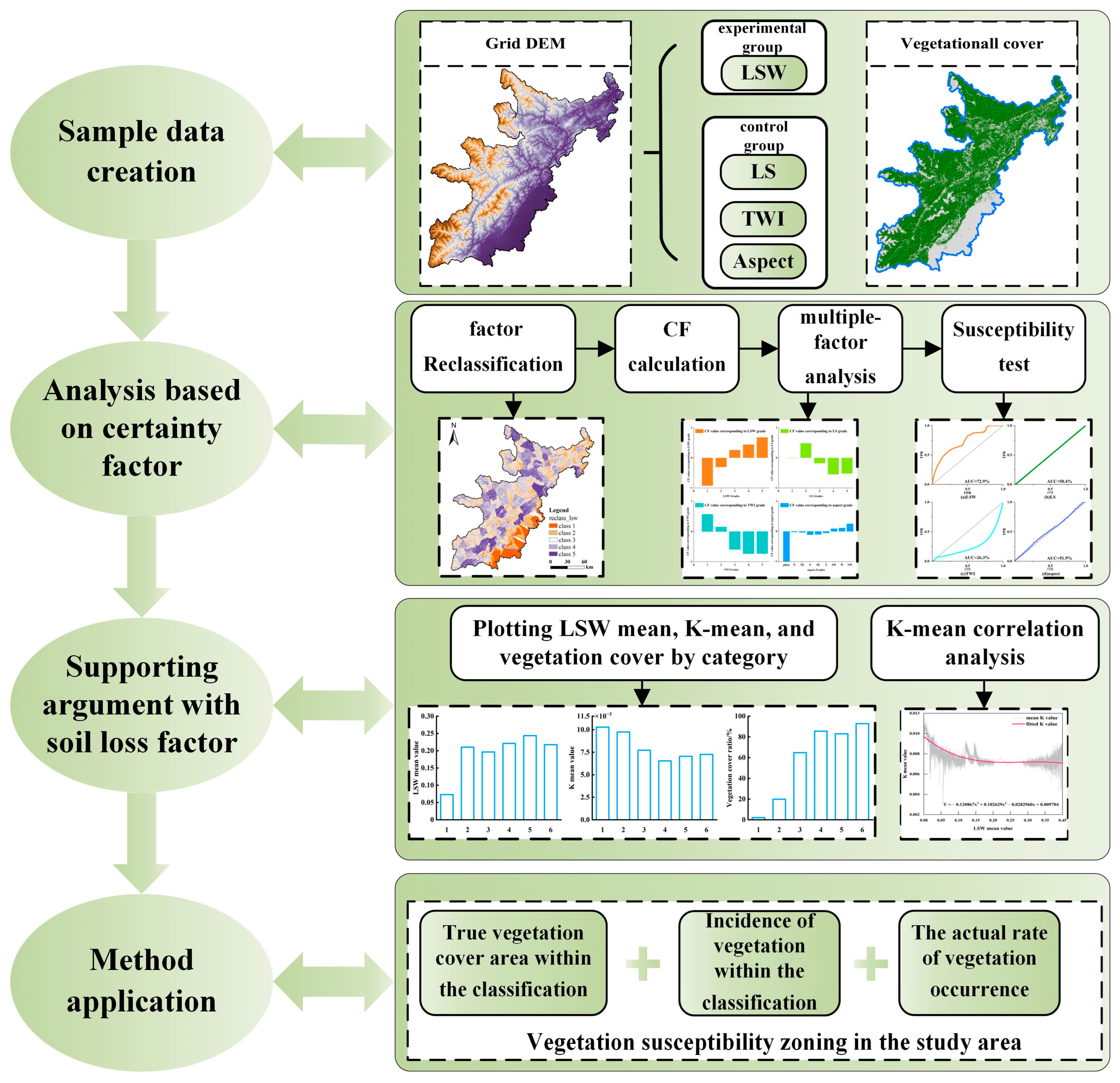
3.4.3. Evaluation Process

To comprehensively explore the relationship between LSW factors and vegetation cover, the evaluation method flow is shown in Figure 4, which is divided into four steps overall.

(1)

Obtain the corresponding topographic factors.

(2)

Based on the tools of reclassification, spatial analysis, and superposition analysis in ArcGIS 10.7, the CF value of each factor level is calculated and then combined with the numerical distribution law to carry out multi-factor impact analysis. After the topographic impacts of the site environment were analyzed, the evaluation of vegetation susceptibility was examined with the help of the Receiver Operating Characteristic (ROC) curve.

(3)

Combined with the distribution characteristics of soil erodibility K values in the study area, qualitative description and correlation analysis were carried out for K and LSW to support the rationality for vegetation cover evaluation by LSW.

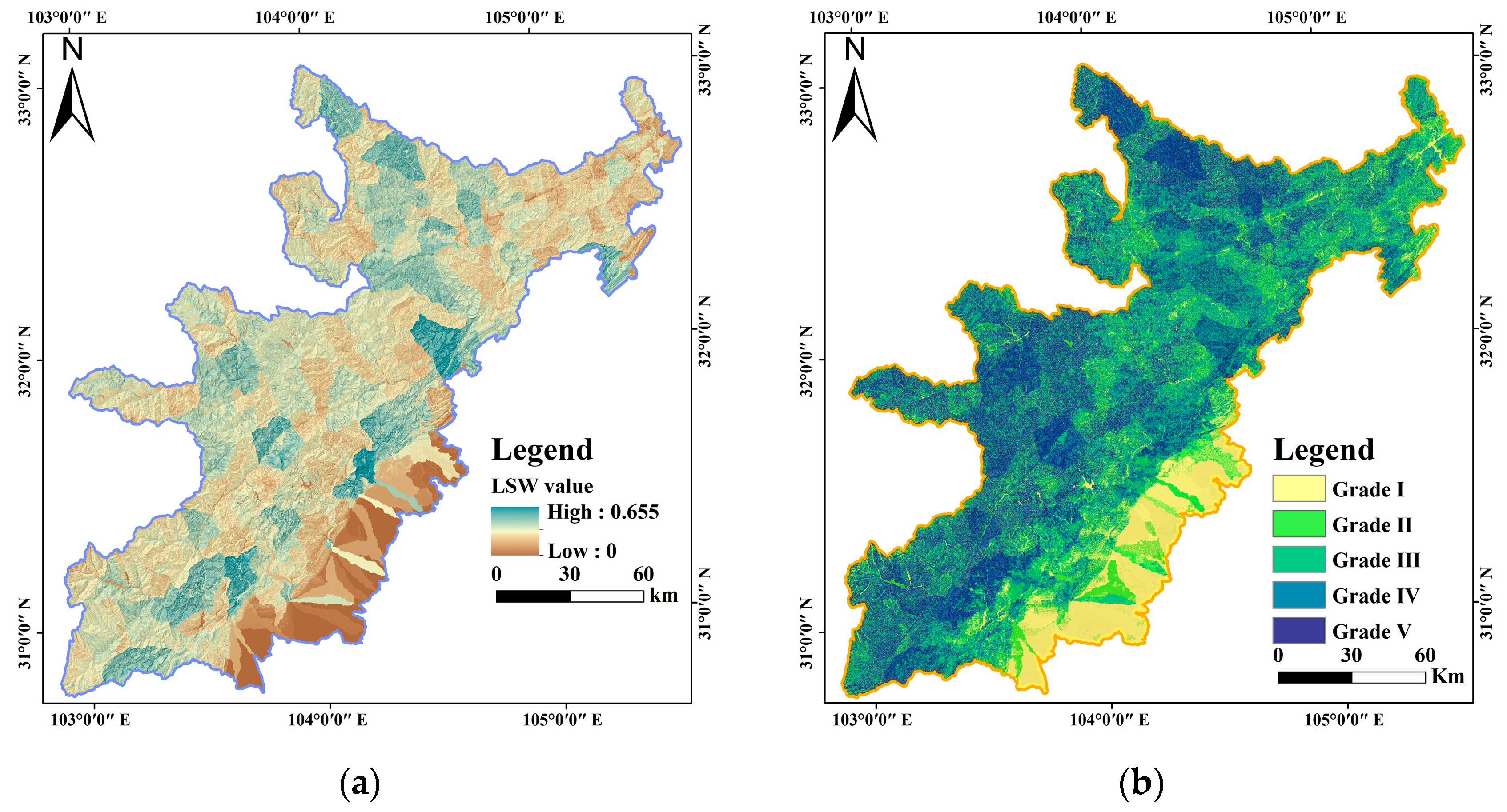
(4)

Obtain the vegetation cover susceptibility zoning map of the study area, and also use the indicators A (ratio of the area of this susceptibility class to the total area of the study area), B (ratio of the vegetation within this susceptibility class to total vegetation), and the actual vegetation occurrence ratio B/A (the ratio of vegetation density within a certain susceptibility class to that of the total study area) for reliability testing.

4. Results and Discussion

4.1. Multi-Factor Analysis of Vegetation Cover

Taking the DEM of the study area as the foundation, the topographic factors LSW, LS, TWI, and aspect were calculated; subsequently, the reclassification work was carried out. Among them, the slope aspect starts from a clockwise direction and is divided into nine categories according to 45° as the grading interval, and then considering the flat land situation where the slope aspect does not exist. For LSW, LS, and TWI, the natural breaks classification was applied for reclassification. The method adopts a similar idea to clustering, taking the maximum similarity within each group and the maximum difference between different groups as the starting point, while balancing the need for the range and number of elements in various groups to be as close as possible so as to satisfy the reasonable division of each level. Ultimately, LSW, LS, and TWI were all classified into five categories. After the classification was completed, the results of calculating the CF values of each class for each factor are shown in

Table 1. CF values calculated for each class of LSW and control group factors.

Impact Factor	Grade	Total Graded Area/km2	Vegetation Coverage/%	CF
LSW	Ⅰ	2279.97	17.27	−0.92
	Ⅱ	5044.07	66.45	−0.30
	Ⅲ	8210.95	79.39	0.25
	Ⅳ	6942.36	83.66	0.44
	Ⅴ	3700.43	89.95	0.68
LS	Ⅰ	25,807.17	73.97	−0.007
	Ⅱ	356.12	84.75	0.48
	Ⅲ	12.00	70.02	−0.18
	Ⅳ	2.11	56.22	−0.55
	Ⅴ	0.40	57.64	−0.52
TWI	Ⅰ	10,255.48	86.07	0.56
	Ⅱ	9427.70	77.17	0.15
	Ⅲ	4647.56	53.83	−0.59
	Ⅳ	1405.18	43.05	−0.73
	Ⅴ	441.8	43.33	−0.73
Aspect	Ⅰ(plane)	57.55	0.80	−0.99
	Ⅱ(N)	3124.87	73.74	−0.01
	Ⅲ(NE)	3261.75	73.48	−0.03
	Ⅳ(E)	3966.14	71.82	−0.10
	Ⅴ(SE)	3552.50	72.04	−0.10
	Ⅵ(S)	3262.89	73.04	−0.05
	Ⅶ(SW)	3044.32	75.92	0.09
	Ⅷ(W)	2964.20	76.35	0.11
	Ⅸ(NW)	2943.54	79.31	0.25

.

Synthesizing the data in Table 1, the LSW factor of the experimental group was analyzed versus the factor of the control group, as follows.

(1)

LS and LSW: LS factor as a component of the USLE is directly linked to the hydraulic erosion suffered by the soil, and is more intuitively expressed as a linear correlation; in other words, the larger the LS factor is, the more serious the soil erosion is within the region. Based on the above analysis, the five gradations of LS factors also exhibit a clear regularity. With the division of grade I~V, the CF value shows a tendency to shrink from near zero value to negative value amplification, which is related to the properties of LS itself. In particular, The CF value of grade Ⅳ and Ⅴ in LS reaches −0.5, which had a significant effect on the vegetation growth and development. It was shown that as the LSW factor increased from grade I to V, the corresponding CF values showed a clear pattern of changing from negative to positive values, which was considerably different from the pattern of the LS factor. Compared with the LS factor, the LSW factor not only ensures the reasonable preservation of the fusion information, but also supplements the slope width information to help it express the ground information more thoroughly, which is also empirically supported by the information entropy test [28]. The rules of LSW gradation corresponding to CF in Table 1 are notable, which means the LSW value can effectively determine whether a particular area of land is suitable for vegetation growth.

(2)

TWI: TWI is a measure of soil water content and potential magnitude of runoff occurrence in a certain region. If the TWI is higher in a region, the corresponding saturated zone has a greater potential for development [69]. From the principle of vegetation growth, if the soil is highly saturated with water, it is easy to produce surface runoff. Once the soil remains saturated with water for a long time, the water balance in the vegetation cells is disrupted. This is not conducive to the absorption of plant nutrients such as Ca, K, Mg [74], thus affecting the vegetation growth and development. According to Table 1, the CF value corresponding to TWI decreases gradually as the grade increases, indicating that excessive water saturation in the soil is instead detrimental to the vegetation cover, which is consistent with the vegetation growth law.

(3)

Aspect: As seen in Table 1, the slope aspect of the flat land shows a significant negative effect with vegetation cover. Due to the absence of the slope aspect means that the ground is not deflected in either direction, the vegetation is more likely to be dominated by other factors in such cases. The study period is in the spring to summer transition stage, dominated by the temperate atmospheric mass. However, the study areas with SW, W, and NW aspects showed a positive correlation. After considering the complex factors, the following inference is made: the western part of the study area benefits from the high mountain barrier effect, with more rainfall on the windward side and less rainfall on the leeward side, and the classical rain shadow effect comes into play [75,76]. In addition, soil erosion is serious with rainfall, and insufficient soil depth makes it difficult for vegetation to thrive. Moreover, increased rainfall will increase the leaching of nutrients from the soil [77] and enhance soil acidity [78], so that the windward slopes of the undulating steep mountains will not be a good environment for vegetation growth. The data in Table 1 also confirm the emergence of this phenomenon.

4.2. Vegetation Susceptibility Evaluation and Test

After obtaining the distribution of CF values for each class of potential impact factors in the study area, the idea that LSW is closely related to vegetation cover was proposed from a qualitative perspective, while further demonstration is needed for the quantitative description of LSW that can be used for vegetation cover.

The ROC curve is widely used in the evaluation of medical diagnostic test performance and landslide prediction [79,80]. In the case of single factor evaluation, the susceptibility and specificity at different thresholds can be calculated by constructing a logistic regression model [81]. Afterwards, the ROC curve was plotted with sensitivity as the ordinate and specificity as the abscissa [82]. Among them, susceptibility is the true positive rate (TPR) and specificity is the false positive rate (FPR) (

Table 2. Definition of performance evaluation index.

	Predict Positive	Predict Negative
True positive	True positives (TP)	False negatives (FN)
True negative	False positives (FP)	True negatives (TN)

, reproduced with permission from [82], Elsevier, 2023). The formulas are as follows:

$$\mathrm{TPR}=\frac{\mathrm{TP}}{\mathrm{TP}+\mathrm{FN}}$$

(4)

$$\mathrm{FPR}=\frac{\mathrm{FP}}{\mathrm{FP}+\mathrm{TN}}$$

(5)

The area under curve (AUC) can be used as a gauge of the model prediction accuracy. Intuitively, the ROC curve divides the closed graph of Figure 5 into two parts, and the size of the area below the curve is the AUC. The closer the AUC value is to 1 (or expressed as a percentage, i.e., 100%), the stronger the judgment of the model is [83]. Based on the above analysis, this paper intends to use the ROC curve to prove the correctness and reliability of the evaluation method. After acquiring the raster of vegetation susceptibility evaluation results under the impact factors, the cumulative percentage of susceptible area and the cumulative percentage of actual vegetation occurrence curves were established (seen in Figure 5). It is evident from comparing the AUC values in the four cases that the prediction of vegetation cover based on the LSW factor is the most accurate, with an AUC value of 72.9%; the evaluation of both LS and slope aspect factors is the second most effective with a stable AUC value of about 50%, while the prediction of TWI is the worst with an AUC value of less than 30%. As illustrated by the control group experiments, the LSW factor has a unique advantage in conducting vegetation cover susceptibility evaluation. From the factor theory analysis, the reason for the low success rate of TWI evaluation of vegetation cover distribution may be related to the blockage of groundwater connectivity in arid or semi-arid areas in the study region, which corresponds to the greater spatial heterogeneity of runoff mechanisms between the area and the humid area [69], resulting in the failure to meet the TWI assumptions on soil conditions. Looking at the graded CF values of LSW and TWI in Table 1, the difference in the evaluation success rate between the two factors confirms the strong correlation between vegetation cover and CF values. The evaluation success rate of vegetation cover will similarly rise in step with a positive increase in the CF value.

4.3. Correlation Analysis of Erodibility Factor

Soil erodibility factor (i.e., K value) can measures the extent to which soil properties in the area affect soil erosion [84], and is widely used in soil erosion resistance evaluation and heterogeneity analysis [85,86]. Soil erosion acts profoundly on vegetation growth and development, and by exploring the relationship between K and LSW, the mechanism of action of LSW and vegetation cover can be mapped from the perspective of soil and water conservation.

In order to comprehensively assess the relationship between K and LSW, the six feature areas mentioned in Section 3.2 were selected as the test sites, and the LSW and K values of the corresponding study areas were obtained. The K value data used in this paper were sourced from the National Earth System Science Data Center (Data webpage: http://www.geodata.cn, accessed on 3 February 2023). Following the collection of data, the mean LSW value, mean K value, and vegetation coverage in different test areas were plotted, as shown in a, b, and c of Figure 6, respectively.

4.3.1. Qualitative Relationship Reasoning between LSW and K

According to Figure 6a, the average value of LSW increases gradually during the transition from plains to mountains. This situation may be related to the positive increase in slope length due to the development of the slope body [23]. There is an exponential growth relationship between slope length and slope width [38], so the corresponding LSW value will increase if the slope change is stable. Figure 6c also shows that vegetation coverage remained largely positively expanding during this phase, which is consistent with the results in Table 1. The decrease in mean LSW values during the transition from category 5 to 6 may be due to the disruption of slope ductility by excessive undulation [87], which in turn decreases the level of mean LSW values. Based on Figure 6a,b, the LSW maintains a positive expansion trend over the course of category 1 to 5, while the K mean value changes in the opposite direction. In addition, the status of mean LSW and mean K value change during category 5 to 6 also conforms to the inverse trend. Overall, mean LSW values are roughly negatively correlated with K values, which is highly consistent with the idea that topography has a direct negative effect on K values [88].

Combined with the data in Table 1, it can be seen that as the value of LSW increases, the larger the CF value corresponding to the grade, the larger the vegetation growth potential is. K value serves as a measure of how soil properties affect soil erosion [89], with larger K values being detrimental to vegetation development. The negative correlation between LSW and K values is consistent with the results of the theoretical analysis. Based on Figure 6c, it can be seen that the vegetation coverage and LSW showed a trend of increasing in the same direction as the transition from plains to mountains. This is in agreement with the rule known in Table 1 that LSW has a positive indicative effect on vegetation growth potential.

Upon analysis, the most significant increase in LSW values between the plains to hills transition (i.e., category 1 to 3) is attributed to the significant difference in slope morphology between the plains and hills, as well as the later stage of gully development on the slopes. It was calculated that the decrease of K value in this stage reached a peak value of 0.00256 (t·hm²·h)/(hm²·MJ·mm) (the value decreased from 0.01028 to 0.00772), and the drop amounted to 24.8%. In terms of soil type, the K level was basically converted from loessial soil to purple soil [90], and this change triggered an increase in soil fertility and soil erodibility with a non-negligible effect on the growth of vegetation [91]. Based on the positive role of gullies in modifying the site environment in Section 2, the differences in LSW levels across terrain categories validate the indicative role of this factor for vegetation growth potential. In addition, the most significant amount of vegetation cover increase at this transition stage can be seen in conjunction with Figure 6c, justifying the mechanism analyses.

According to Figure 6b, the mean value of K shows a gradual decrease from the plain to the small rolling mountains (i.e., category 1 to 4), and if the K value and the LSW value show opposite trends, the K value should continue to decrease during the transition from small rolling to medium rolling mountains (i.e., categories 4 to 5). However, the mean value of K in the corresponding part of Figure 6b shows a small rebound, which is contrary to the mean value of LSW in the corresponding area maintaining an increasing trend. Statistically, the standard deviation of the K value corresponding to categories 1 to 6 were 1.27 × 10⁻³, 8.84 × 10⁻⁴, 1.17 × 10⁻³, 1.12 × 10⁻³, 1.95 × 10⁻³, and 1.46 × 10⁻³ (t·hm²·h)/(hm²·MJ·mm), and the Coefficients of Variation (CV) of the K value for categories 1 to 6 were 0.12, 0.09, 0.15, 0.17, 0.27, and 0.20, respectively. It is evident that the standard deviation and CV of the K value was the largest in the medium rolling hills, with the coefficient of variation above the moderate level [92]. It suggests that this type of terrain has a high degree of soil erosion differentiation. Studies have already pointed out that changes in geomorphology can lead to changes in soil physicochemical properties [92], which ultimately affects the value of K. Therefore, it could be assumed that there is a strong correlation between soil erosion variability and topographic differentiation in the middle rolling hills, so the rebound of the K value during the transition from area 4 to area 5, which can therefore be interpreted as the result of topographic divergence. Moreover, the study area has experienced earthquake hazards. The surface remodeling induced by earthquake has a more intuitive impact on topographic divergence [93,94], which confirms the correctness of the hypothesis.

In terms of the above regional analysis, the LSW value and K value can be preliminarily judged to be negatively correlated. In addition, analysis of Figure 6b,c shows that the greater the level of K values, the higher the degree of soil erosion and the lower the vegetation cover tends to be. Although there are some local limitations to the interpretation of soil erosion status using the mean LSW, it can still broadly explain the vegetation development tendency for medium and large rolling mountains with relatively complex topographic differentiation.

4.3.2. Expression and Analysis of the Quantitative Relationship between LSW and K

To quantitatively describe the relationship between K and LSW, the association between the mean value of LSW and K was calculated based on the data from the six experimental areas, as shown in Figure 7. It is evident from the observation that as the LSW rises, the K value tends to decrease accordingly, which is in agreement with the qualitative analysis of the slope width mechanism and the distribution pattern of CF values corresponding to LSW in Table 1.

Further, as the LSW value increases from 0 to 0.2, the decrease rate of K becomes slower. This pattern can be illustrated in Figure 6: categories 2 to 5 in Figure 6a are in a phase of growth in LSW values, while the shrinking trend in the K value is gradually moderating.

When the LSW value is in the range of 0.2~0.3, the K value tends to be stable. Together with Figure 6a, it can be seen that the elevated LSW values basically represent a change in the slope development. A study has pointed out that when precipitation conditions are stable, the width-to-depth ratio of slope gullies tends to first decrease and then increase with slope development [23]. In terms of geometric characteristics, when the slope length increases, the slope width increases due to lateral erosion [38], whereas increasing rate of slope relative to the slope width shows a dynamic change of first increasing and then decreasing. This can be interpreted as an increase in slope runoff volume with a concomitant decrease in runoff velocity, so that the change in sediment yield is not significant [23,95], which triggers the stabilization of the K value in the phase. During this stage, vegetation growth may be more related to other factors such as temperature and rainfall in the local site environment.

If the mean LSW value continues to increase and exceeds 0.30, the K value will revert to a decreasing trend, correlating with runoff degradation as the slope develops to a certain level [96]. Moreover, a study conducted in the mountainous region of Yunnan, China, showed that the K values decreased significantly for slopes greater than 15° [97]. This finding is partially consistent with the overall trend of the K value. In general, Figure 7 still obeys the pattern of decreasing average erosion rate with slope development, which in turn has a dynamic effect on vegetation growth.

According to the SPSS software (https://www.ibm.com/cn-zh/spss), there is a highly significant negative correlation between LSW and K values (p < 0.01), with a correlation coefficient of −0.388. This quantitative relationship has never been proposed in the past. The negative correlation coefficient asserts that LSW is an important factor influencing the K value, which is a good indication for describing the resistance of soil to water erosion. Regarding the direct impact of the K value on soil erosion, the validity of the LSW factor’s feedback on vegetation growth and development was also sideways confirmed.

4.4. Method Application

The final acquisition of the overall LSW distribution of the study area is shown in Figure 8a. In the previous analysis, the higher the value of LSW factor, the higher the possibility of vegetation cover in the corresponding grid cell. The LSW distribution map in the study area was reclassified using the natural breaks classification commonly used in statistics, and finally divided into five grades, arranged from smallest to largest possibility corresponding to grade Ⅰ to V. The higher the level, the higher the possibility of vegetation occurrence. The different levels of susceptibility correspond to very low, low, medium, high, and very high, in order, and the vegetation susceptibility zoning map is displayed in Figure 8b.

In terms of intuitive distribution, the susceptibility level in the southeastern part of the study area is lower, and can be judged on the basis of LSW that the vegetation distribution here is less dense than in other regions. The study area can be roughly divided into northern, central and southern parts based on latitude range. In the northern and southern parts, the vegetation susceptibility class in the western region is clearly higher than that in the eastern part, while the central region shows an even distribution of vegetation between the eastern and western sides. After comparing the river data in the test area, it was discovered that the eastern part of the central region is a convergence area of water systems such as the Baicao River, Tongkou River, Anchang River, and Kai River. With fertile soil, the vicinity of the water system is often a deep-cut canyon zone [98]. Moreover, soil water content in the canyon zone has a significant positive correlation with soil microbial biomass carbon and nitrogen as well as soil enzyme activities [99], thus producing an effect on vegetation development. Overall, the susceptibility level in the west was higher than that in the east, so the comprehensive conditions in the west were judged to be more suitable for vegetation growth. The corresponding data were obtained by overlaying and analyzing the graded susceptibility classes with the actual vegetation cover distribution data, as shown in

Table 3. Comparison of susceptibility level zoning and actual vegetation distribution data.

Susceptibility Level	LSW Value Range	Graded Area/km2	Vegetation Cover Area/km2	Vegetation Coverage/%	A/%	B%	B/A
Ⅰ	0~0.08955	2279.97	393.95	17.27	8.71	2.03	0.2331
Ⅱ	0.08955~0.18931	5044.07	3352.20	66.45	19.27	17.28	0.8967
Ⅲ	0.18931~0.26861	8210.95	6519.02	79.39	31.37	33.60	1.0711
Ⅳ	0.26861~0.35558	6942.36	5808.06	83.66	26.52	29.93	1.1286
Ⅴ	0.35558~0.65487	3700.43	3328.77	89.95	14.13	17.16	1.2144
Total		26,177.81	19,402.02		100	100

Note: (1) A is the percentage of the area designated with a certain susceptibility class to the total area of the study area; (2) B is the percentage of vegetation within the designated susceptibility class to the total vegetation.

. With the combination of Table 3, it can be seen that the vegetation coverage differs significantly in different susceptibility classes, demonstrating a clear regularity with the increase of classes. The shift from 17.27% vegetation coverage in susceptibility grade I to more than 80% in grades IV and V also confirms the validity of the susceptibility class zoning map. In order to more directly assess the reliability of the rank zoning maps, this paper derives the actual vegetation occurrence rate B/A from the actual landslide ratio [71,100], which is commonly used in the field of landslide susceptibility assessment. The physical significance of this ratio is that it reflects the relationship between the frequency of vegetation occurrence and the conditions under which it is likely to occur [101]. A higher occurrence rate (B/A > 1) indicate that more vegetation events have happened than are likely to occur, suggesting that a high likelihood of occurrence exists, while the opposite is true for a relatively low likelihood of occurrence of vegetation on the surface. Based on Table 3, it can be seen that as the susceptibility level gradually increases, the ratio B/A increases simultaneously. The B/A value increased from the initial 0.23 to about 1.21, and the actual occurrence ratio of vegetation increased nearly six times, indicating that the obtained susceptibility class matches the actual vegetation occurrence and the classification result is more satisfactory. Statistically, the vegetation cover in grades IV and V accounts for 47% of the total vegetation cover area, making up almost half of it. This result suggests that LSW is instructive for vegetation susceptibility, and also reaffirms the validity and authenticity of its zoning. The comprehensive experiment reveals that the ranges of LSW favorable for vegetation occurrence in the study area are above 0.26, and the value intervals in Table 3 can be used as a reference for assessing the regional vegetation growth potential.

5. Summary

Given that the majority of the existing vegetation indices use optical images as data sources, the two-dimensional indicators obtained are challenging to express the spatial heterogeneity of complex three-dimensional structures [102]. This problem is more pronounced in mountainous cities [103], and the use of topographic factor for the expression can somewhat ameliorate this shortcoming.

In this study, the integrated slope factor LSW was found to be highly regular in revealing vegetation growth potential. Through the introduction of the Certainty Factor, the application of LSW for vegetation coverage assessment was proved to be reliable after a control group test. At the same time, the mechanism of LSW acting on vegetation growth proved to be correct. In addition, LSW can effectively delineate the vegetation susceptibility zoning maps of the 10 counties (cities) in Sichuan Province, and the vegetation coverage in the high and very high susceptibility zones accounts for more than 80%, confirming that the results of the assessment are true and credible. In particular, the values range of LSW greater than 0.26 can be used as a reference for delineating regional areas of vigorous vegetation growth.

In the process of exploring the association between LSW and vegetation coverage, the indicative relationship between LSW and soil erosion was additionally revealed. For the range of 10 counties (cities) in Sichuan Province, there is a highly significant negative correlation between LSW and K. When LSW lies in the interval of 0 to 0.2, there is a significant decrease in the value of K. With LSW locates at the level of 0.2 to 0.3 values, the K value will remain stable. As the LSW value is greater than 0.3, the K value will show a gradual downward trend.

In summary, the correlation between slope development, erosion, and vegetation growth can provide corresponding decision-making knowledge in the fields of erosion control and ecological restoration. With the increasing public availability of DEM, scholars can easily access DEMs in different time domains and carry out numerical dynamic supervision of LSW in the study area. In the event that a staged change in LSW is detected, early warning or contingency measures can be provided in a timely manner. For example, when a sharp decrease in LSW values is monitored in a localized area, it reflects the drastic fluctuation of soil erosion in this range, and the frequency of soil physicochemical property supervision should be increased at this time in order to prevent gully wall collapses or landslide disasters from occurring [23]. For the field of ecological management, LSW numerical monitoring can provide recommendations for ecological restoration. For instance, when delineating the area of planted forests, priority can be given to areas with large LSW values. Artificial interventions such as mechanical sand barriers [104] and artificial sand fields [105] can be implemented in areas with small LSW values, which provide a certain reference value for guaranteeing the recovery of ecological functions.

Although this study is enlightening, there are some limitations:

(1)

This method has not been compared with other methods for assessing vegetation growth potential, and the superiority of this method remains to be examined.

(2)

The research methodology was tested only within 10 counties in Sichuan Province, and extension to other regions for validation will allow the methodology’s suitability to be tested.

(3)

In this paper, the correlation between LSW and vegetation cover was demonstrated by using the certainty factor, but the success rate of vegetation cover appraisals by LSW alone is still limited. Considering the completeness of the evaluation system, it is possible to add other elements such as net shortwave radiation flux at the Earth’s surface to improve the reliability and completeness of the evaluation method, and how to construct a new evaluation index with LSW as the main body will become the research direction in the future.

References

1. Gemitzi, A.; Albarakat, R.; Kratouna, F.; Lakshmi, V. Land cover and vegetation carbon stock changes in Greece: A 29-year assessment based on CORINE and Landsat land cover data. Sci. Total Environ. 2021, 786, 147408. [Google Scholar] [CrossRef] [PubMed]
2. Zhan, X.G.; Wang, P. Research on dynamical supervision design of water and soil loss in Three Gorges reservoir area based on RS and GIS. J. Yangtze River Sci. Res. Inst. 2001, 18, 41–44. [Google Scholar]
3. Li, M.M. The Method of Vegetation Fraction Estimation by Remote Sensing. Master’s Thesis, Institute of Remote Sensing Applications Chinese Academy of Sciences, Beijing, China, 2003. [Google Scholar]
4. Feng, X.H.; Zeng, Z.L.; Jing, M.X.; Gao, K.C.; Xiao, Y.Q. Influence of driving factors under different vegetation indices of NDVI and EVl in Guangdong-Hong Kong-Macao Greater Bay Area. J. Huazhong Agric. Univ. 2023, 42, 116–124. [Google Scholar] [CrossRef]
5. Chen, H.; Huang, W.; Li, W.; Niu, Z.; Zhang, L.; Xing, S. Estimation of LAI in Winter Wheat from Multi-Angular Hyperspectral VNIR Data: Effects of View Angles and Plant Architecture. Remote Sens. 2018, 10, 1063. [Google Scholar]
6. Wang, Z.X.; Liu, C.; Alfredo, H. From AVHRR-NDVI to MODIS-EVI: Advances in vegetation index research. Acta Ecol. Sin. 2003, 23, 979–987. [Google Scholar]
7. Purevdorj, T.S.; Tateishi, R.; Ishiyama, T.; Honda, Y. Relationships between percent vegetation cover and vegetation indices. Int. J. Remote Sens. 1998, 19, 3519–3535. [Google Scholar] [CrossRef]
8. Correa-Díaz, A.; Romero-Sánchez, M.E.; Villanueva-Díaz, J. The greening effect characterized by the Normalized Difference Vegetation Index was not coupled with phenological trends and tree growth rates in eight protected mountains of central Mexico. For. Ecol. Manag. 2021, 496, 119402. [Google Scholar] [CrossRef]
9. Coulthard, B.L.; Touchan, R.; Anchukaitis, K.J.; Meko, D.M.; Sivrikaya, F. Tree growth and vegetation activity at the ecosystem-scale in the eastern Mediterranean. Environ. Res. Lett. 2017, 12, 084008. [Google Scholar] [CrossRef]
10. Tang, G.A.; Li, F.Y.; Liu, X.J. Digital Elevation Model Tutorial; Science Press: Beijing, China, 2016; p. 241. [Google Scholar]
11. Zhou, F.B.; Ma, G.W.; Xie, C.C.; Yang, Z.Q.; Zhong, S.P. Research of compound terrain factors extraction based on BP neural network. Sci. Surv. Mapp. 2023, 48, 227–235. [Google Scholar] [CrossRef]
12. Sun, L.J.; Zhao, D.; Zhang, G.Z.; Wu, X.J.; Yang, Y.; Wang, Z.W. Using SPOT VEGETATION for analyzing dynamic changes and influencing factors on vegetation restoration in the Three-River Headwaters Region in the last 20 years (2000–2019), China. Ecol. Eng. 2022, 183, 106742. [Google Scholar] [CrossRef]
13. Beale, J.; Grabowski, R.C.; Lokidor, P.L.; Vercruysse, K.; Simms, D.M. Vegetation cover dynamics along two Himalayan rivers: Drivers and implications of change. Sci. Total Environ. 2022, 849, 157826. [Google Scholar] [CrossRef] [PubMed]
14. Xiong, Y.L.; Li, Y.R.; Xiong, S.Y.; Wu, G.H.; Deng, O.P. Multi-scale spatial correlation between vegetation index and terrain attributes in a small watershed of the upper Minjiang River. Ecol. Indic. 2021, 126, 107610. [Google Scholar] [CrossRef]
15. Li, Q.; Shi, X.Y.; Wu, Q.Q. Exploring suitable topographical factor conditions for vegetation growth in Wanhuigou catchment on the Loess Plateau, China: A new perspective for ecological protection and restoration. Ecol. Eng. 2020, 158, 106053. [Google Scholar] [CrossRef]
16. Ma, S.; Qiao, Y.P.; Wang, L.J.; Zhang, J.C. Terrain gradient variations in ecosystem services of different vegetation types in mountainous regions: Vegetation resource conservation and sustainable development. For. Ecol. Manag. 2021, 482, 118856. [Google Scholar] [CrossRef]
17. Wu, J.; Wang, G.; Chen, W.; Pan, S.; Zeng, J. Terrain gradient variations in the ecosystem services value of the Qinghai-Tibet Plateau, China. Glob. Ecol. Conserv. 2022, 34, e02008. [Google Scholar] [CrossRef]
18. Ochoa, P.A.; Fries, A.; Mejia, D.; Burneo, J.I.; Ruiz-Sinoga, J.D.; Cerda, A. Effects of climate, land cover and topography on soil erosion risk in a semiarid basin of the Andes. Catena 2016, 140, 31–42. [Google Scholar] [CrossRef]
19. Jin, F.M.; Yang, W.C.; Fu, J.X.; Li, Z. Effects of vegetation and climate on the changes of soil erosion in the Loess Plateau of China. Sci. Total Environ. 2021, 773, 145514. [Google Scholar] [CrossRef]
20. Zhang, Y.; Zhang, D.J. Improvement of terrain niche index model and its application in vegetation cover evaluation. Acta Geogr. Sin. 2022, 77, 2757–2772. [Google Scholar]
21. Huang, B.W.; Zha, R.B.; Mao, L.H.; Wu, J.L.; Liu, J.M. Evolution of Soil and Water Conservation Benefits in the Process of Vegetation Restoration on Slope of Eroded and Degraded Red Soil. J. Soil Water Conserv. 2022, 36, 135–142. [Google Scholar] [CrossRef]
22. Wang, K.; Zhou, J.; Tan, M.L.; Lu, P.; Xue, Z.; Liu, M.; Wang, X. Impacts of vegetation restoration on soil erosion in the Yellow River Basin, China. Catena 2024, 234, 107547. [Google Scholar] [CrossRef]
23. Gou, J.F.; Gan, F.L.; Liu, C.H. Variation of Rill Morphology and lts Effect on Runoff and Sediment Yield on Purple Soil Slope. Res. Soil Water Conserv. 2023, 30, 61–68+75. [Google Scholar] [CrossRef]
24. Yang, X.; Tang, G.A.; Yuan, B.Y.; Liu, H.L.; Huang, X.L.; Li, C.R. Characteristics and development process of spoon-shaped gully in the Loess Plateau. Geogr. Res. 2021, 40, 1870–1886. [Google Scholar]
25. Ni, J.P.; Wei, C.F.; Xie, D.T.; Gao, M.; He, B.H. Influence of slope gradient on runoff erosion of purple soil slope in the Three Gorges Reservoir area. J. Sediment Res. 2009, 2, 29–33. [Google Scholar] [CrossRef]
26. Su, Y.Y.; Li, P.; Ren, Z.P.; Xiao, L.; Wang, T.; Zhang, J.W.; Liu, Z. Effect of Slope Gradient on the Process of Runoff and Sediment Yield and Water-Sediment Relation on the Loess Slope. Res. Soil Water Conserv. 2020, 27, 118–122. [Google Scholar] [CrossRef]
27. Tan, J.B.; Zuo, J.Q.; Xie, X.Y.; Ding, M.Q.; Xu, Z.K.; Zhou, F.B. MLAs land cover mapping performance across varying geomorphology with Landsat OLI-8 and minimum human intervention. Ecol. Inform. 2021, 61, 101227. [Google Scholar] [CrossRef]
28. Zhou, F.B.; Xie, C.C.; Wang, J.; Chen, B.L.; Hu, Y. Slope body factor fusion of grid DEM. Bull. Surv. Mapp. 2022, 104–109. [Google Scholar] [CrossRef]
29. Lu, H.X.; Liu, X.J.; Tang, G.A. Terrain Complexity Assessment Based on Multivariate Analysis. Mt. Res. 2012, 30, 616–621. [Google Scholar] [CrossRef]
30. Mo, F. The Application of WEPP and GIS. Master’s Thesis, Xi’an University of Technology, Xi’an, China, 2004. [Google Scholar]
31. Cochrane, T.A.; Flanagan, D.C. Assessing water erosion in small watersheds using WEPP with GIS and digital elevation models. J. Soil Water Conserv. 1999, 54, 678–685. [Google Scholar]
32. Li, Y.L.; Wang, L.S.; Wang, T.H. Moisture migration of unsaturated soil due to matric suction gradients. J. Xi’an Univ. Archit. Technol. 2017, 49, 847–851+859. [Google Scholar] [CrossRef]
33. Wainwright, J.; Turnbull, L.; Ibrahim, T.G.; Lexartza-Artza, I.; Thornton, S.F.; Brazier, R.E. Linking environmental régimes, space and time: Interpretations of structural and functional connectivity. Geomorphology 2011, 126, 387–404. [Google Scholar] [CrossRef]
34. Hao, H.X.; Guo, Z.L.; Li, Z.X.; Hua, L. Characteristics of Rill Cross-Section Morphology and Hydrodynamics on Red Soil Slope. Resour. Environ. Yangtze Basin 2018, 27, 363–370. [Google Scholar]
35. Jin, X.; Liu, H.N.; Song, Y.; Zhai, T.; Zhao, Z.X.; Shi, W.F. Changes of the channel geometric characteristics during the development of rills to shallow ditches. China Rural. Water Hydropower 2022, 8–16. [Google Scholar]
36. Li, W.Q.; Wen, X.X.; Gao, M.S.; Xiong, X.R. Studies on Water and Physiological Effect of Winter Wheat with Plastic Film Mulching in Semiarid Farmland. Acta Agric. Boreali-Occident. Sin. 2008, 17, 146–151. [Google Scholar]
37. Guan, F.C.; Miao, Y.J.; Fang, T.B.; Lan, X.Z.; Liang, Z.W. Effects of Ridging on Soil and Above-ground Biomass in Heavy Alkal-i saline Grasslands of West Songnen Plain China. Acta Agrestia Sin. 2010, 18, 763–767. [Google Scholar]
38. Khalaf, H.S.; Mustafa, Y.T.; Fayyadh, M.A. Digital Mapping of Soil Organic Matter in Northern Iraq: Machine Learning Approach. Appl. Sci. 2023, 13, 10666. [Google Scholar] [CrossRef]
39. Vidya, P.V.; Rajathy, S.; Kumar, C.S.R. Composition of sedimentary organic matter in Thrissur Kole wetland, southwest India. Environ. Earth Sci. 2023, 82, 174. [Google Scholar] [CrossRef]
40. Ministry of Land and Resources of the People’s Republic of China. Ten Counties and Cities, Including Wenchuan, Were Assessed as Extremely Hard-Hit Areas. Available online: http://www.npc.gov.cn/zgrdw/npc//zt/2008-07/23/content_1438768.htm (accessed on 2 February 2023).
41. Yin, L.; Wang, L.; Li, T.; Lu, S.; Tian, J.; Yin, Z.; Li, X.; Zheng, W. U-Net-LSTM: Time Series-Enhanced Lake Boundary Prediction Model. Land 2023, 12, 1859. [Google Scholar] [CrossRef]
42. Han, X.S.; Xu, H.; Cai, J.J.; Dong, L.G.; Guo, Y.Z.; An, Y.; Wan, H.X.; Wang, Y.L. Effects of Site Factor and Coverage on Soil Moisture of Maize Field in Zhongzhuang Small Watershed in the Loess Area of Southern Ningxia. Res. Soil Water Conserv. 2023, 30, 112–122. [Google Scholar] [CrossRef]
43. Qiu, Y.; Fu, B.; Wang, J.; Chen, L. Soil moisture variation in relation to topography and land use in a hillslope catchment of the Loess Plateau, China. J. Hydrol. 2001, 240, 243–263. [Google Scholar] [CrossRef]
44. Zhai, T.L.; Jin, G.; Deng, X.Z.; Li, Z.H.; Wang, Y. Study of vegetation information extraction method based on Landsat8 satellite images. Sci. Surv. Mapp. 2016, 41, 126–131+158. [Google Scholar] [CrossRef]
45. Cheng, S.Y.; Cao, S.K.; Cao, G.C.; Han, J.P.; Han, G.Z.; Wu, F.T. Comparisons of Supervised Classification Methods for Land Cover Based on High Spatial Resolution Remote Sensing lmages in Shaliu River Basin of Qinghai Lake. Bull. Soil Water Conserv. 2018, 38, 261–268+353. [Google Scholar] [CrossRef]
46. Sun, J.; Yang, J.; Zhang, C.; Yun, W.; Qu, J. Automatic remotely sensed image classification in a grid environment based on the maximum likelihood method. Math. Comput. Model. 2013, 58, 573–581. [Google Scholar] [CrossRef]
47. Cheng, G.Q.; Wang, Z.Y.; Chen, H. Accuracy Comparison of Landsat-8 Supervised Classifier:Taking Huangdao District as an Example. Geomat. Spat. Inf. Technol. 2019, 42, 146–148+151+155. [Google Scholar]
48. Ali, M.Z.; Qazi, W.; Aslam, N. A comparative study of ALOS-2 PALSAR and landsat-8 imagery for land cover classification using maximum likelihood classifier. Egypt. J. Remote Sens. Space Sci. 2018, 21, S29–S35. [Google Scholar] [CrossRef]
49. Guo, L.N.; Zhang, M.H.; Zhang, Y.B.; Niu, Z.G.; Li, M.Q. Land use hierarchical classification based on Landsat 8 image in Tangshan city. Sci. Surv. Mapp. 2017, 42, 88–94+125. [Google Scholar] [CrossRef]
50. Yin, L.; Wang, L.; Li, T.; Lu, S.; Yin, Z.; Liu, X.; Li, X.; Zheng, W. U-Net-STN: A Novel End-to-End Lake Boundary Prediction Model. Land 2023, 12, 1602. [Google Scholar] [CrossRef]
51. Cheng, W.M.; Zhou, C.H.; Chai, H.X.; Zhao, S.M.; Li, B.Y. Quantitative Extraction and Analysis of Basic Morphological Types of Land Geomorphology in China. J. Geo-Inf. Sci. 2009, 11, 725–736. [Google Scholar] [CrossRef]
52. Li, Z.M.; Chang, Y.Y.; Zhao, Y.F.; Zhang, L.Y. DEM-based Geomorphological Classification and Quantitative Analysis in the Tongbai Mountain Area. J. Xinyang Norm. Univ. 2021, 34, 83–87. [Google Scholar]
53. Yang, Q.K.; Guo, W.L.; Zhang, H.M.; Wang, L.; Cheng, L.; Li, J. Method of Extracting LS Factor at Watershed Scale Based on DEM. Bull. Soil Water Conserv. 2010, 30, 203–206+211. [Google Scholar] [CrossRef]
54. Liu, B.; Xiaogang, B.; Suhua, F. Beijing Soil Loss Equation; Science Press: Beijing, China, 2010; p. 184. [Google Scholar]
55. Liu, B.; Nearing, M.; Risse, M. Slope Gradient Effects on Soil Loss for Steep Slopes. Trans. ASAE 1994, 37, 1835–1840. [Google Scholar] [CrossRef]
56. Yao, B.G.; Zhou, W.B. Research on hydrological characteristics extraction of Chanba Basin based on DEM and ArcGIS. J. Water Resour. Water Eng. 2017, 28, 8–13. [Google Scholar]
57. Li, Y.P. Study on Soil Erosion Simulation Based on GeoWEPP in Western Mining Area. Master’s Thesis, China University of Mining and Technology, Xuzhou, China, 2018. [Google Scholar]
58. Shortliffe, E.H.; Buchanan, B.G. A model of inexact reasoning in medicine. Math. Biosci. 1975, 23, 351–379. [Google Scholar] [CrossRef]
59. Heckerman, D. Probabilistic interpretations for mycin’s certainty factors. In Machine Intelligence and Pattern Recognition; Kanal, L.N., Lemmer, J.F., Eds.; North-Holland: Amsterdam, The Netherlands, 1986; Volume 4, pp. 167–196. [Google Scholar]
60. Arabameri, A.; Pradhan, B.; Rezaei, K. Gully erosion zonation mapping using integrated geographically weighted regression with certainty factor and random forest models in GIS. J. Environ. Manag. 2019, 232, 928–942. [Google Scholar] [CrossRef] [PubMed]
61. Chen, L.H.; Li, L.F.; Wu, F.; Xu, Y.X. Evaluation of the Geological Hazard Vulnerability in the Beiliu City Based on GlS and Information Value Model. Earth Environ. 2020, 48, 471–479. [Google Scholar] [CrossRef]
62. Chen, Z.; Liang, S.; Ke, Y.; Yang, Z.; Zhao, H. Landslide susceptibility assessment using evidential belief function, certainty factor and frequency ratio model at Baxie River basin, NW China. Geocarto Int. 2019, 34, 348–367. [Google Scholar] [CrossRef]
63. Fan, W.; Wei, X.-s.; Cao, Y.-b.; Zheng, B. Landslide susceptibility assessment using the certainty factor and analytic hierarchy process. J. Mt. Sci. 2017, 14, 906–925. [Google Scholar] [CrossRef]
64. Wischmeier, W.H.; Smith, D.D. Predicting rainfall erosion losses: A guide to conservation planning. In Agriculture Handbook; Department of Agriculture, Science and Education Administration: Washington, DC, USA, 1978. [Google Scholar]
65. Williams, J.R.; Berndt, H. Sediment yield prediction based on watershed hydrology. Trans. ASABE 1977, 20, 1100–1104. [Google Scholar] [CrossRef]
66. Renard, K.G.; Ferreira, V.A. RUSLE Model Description and Database Sensitivity. J. Environ. Qual. 1993, 22, 458–466. [Google Scholar] [CrossRef]
67. Liu, B.; Yun, X.; Keli, Z. Soil Erosion Prediction Model; China Science and Technology Press: Beijing, China, 2001; p. 252. [Google Scholar]
68. Kaffas, K.; Pisinaras, V.; Al Sayah, M.J.; Santopietro, S.; Righetti, M. A USLE-based model with modified LS-factor combined with sediment delivery module for Alpine basins. Catena 2021, 207, 17. [Google Scholar] [CrossRef]
69. Zhang, C.X.; Yang, Q.K.; Li, R. Advancement in Topographic Wetness Index and Its Application. Prog. Geogr. 2005, 24, 116–123. [Google Scholar]
70. Luo, Z.F.; Pu, D.C.; Xie, H.B.; Tan, D.J. Landslide Hazard Evaluation in Debris Flow Catchment Area Based on GIS and Information Method. China Saf. Sci. J. 2011, 21, 144–150. [Google Scholar] [CrossRef]
71. Gao, K.C.; Cui, P.; Zhao, C.Y.; Wei, F.Q. Landslide hazard evaluation of wanzhou based on gis information value method in the three gorges eservoir. Chin. J. Rock Mech. Eng. 2006, 21, 991–996. [Google Scholar]
72. Dharmawan, I.W.; Pratiwi; Siregar, C.A.; Narendra, B.H.; Undaharta, N.K.; Sitepu, B.S.; Sukmana, A.; Wiratmoko, M.D.; Abywijaya, I.K.; Sari, N. Implementation of Soil and Water Conservation in Indonesia and Its Impacts on Biodiversity, Hydrology, Soil Erosion and Microclimate. Appl. Sci. 2023, 13, 7648. [Google Scholar] [CrossRef]
73. Lan, H.X.; Wu, F.Q.; Zhou, C.H.; Wang, S.J. Analysis On Susceptibility Of Gis Based Landslide Triggering Factors In Yunnan Xiaojiang Watershed. Chin. J. Rock Mech. Eng. 2002, 21, 1500–1506. [Google Scholar]
74. Jin, X.L.; Zhao, W.; Li, M.D.; Liu, D.D.; Ju, W.L. Effects of soil moisture on the stoichiometric characterist of aboveground plants following conversion of farmland to grassland on the loess plateau. Res. Soil Water Conserv. 2022, 29, 57–63. [Google Scholar] [CrossRef]
75. Chen, C.F.; Hu, B.J.; Li, Y.Y. Easy-to-use spatial random-forest-based downscaling-calibration method for producing precipitation data with high resolution and high accuracy. Hydrol. Earth Syst. Sci. 2021, 25, 5667–5682. [Google Scholar] [CrossRef]
76. Padmakumari, B.; Maheskumar, R.S.; Harikishan, G.; Morwal, S.B.; Kulkarni, J.R. Rain-shadow: An area harboring “Gray Ocean” clouds. Atmos. Res. 2018, 205, 70–79. [Google Scholar] [CrossRef]
77. Song, J.H.; Her, Y.; Yu, X.Y.; Li, Y.C.; Smyth, A.; Martens-Habbena, W. Effect of information-driven irrigation scheduling on water use efficiency, nutrient leaching, greenhouse gas emission, and plant growth in South Florida. Agric. Ecosyst. Environ. 2022, 333, 107954. [Google Scholar] [CrossRef]
78. Zhu, X.; Yang, Z.; Zheng, J.; Liu, J.; Bu, F.; Dai, C.; Lu, Y. Study on Mechanical Properties of Sulfate Saline Soil Improved by CLI-Type Polymer Active Agent. App. Sci. 2023, 13, 10727. [Google Scholar] [CrossRef]
79. Sun, D.; Gu, Q.; Wen, H.; Xu, J.; Zhang, Y.; Shi, S.; Xue, M.; Zhou, X. Assessment of landslide susceptibility along mountain highways based on different machine learning algorithms and mapping units by hybrid factors screening and sample optimization. Gondwana Res. 2022, 123, 89–106. [Google Scholar] [CrossRef]
80. The Collaborative Research Group of the National 10th Five Year Plan Project: A Study on Evaluation and Intervention of the Coronary Heart Disease and Stroke Integrated Risk. A study on evaluation of the risk of ischemic cardiovascular diseases in Chinese and the development of simplified tools for the evaluation. Chin. J. Cardiol. 2003, 30, 16–24. [Google Scholar]
81. Ma, X.D. Application of LiDAR Technology in Geological Hazard Identification and Susceptibility Assessment of Jiuzhaigou Landslide. Master’s Thesis, Southwest University of Science and Technology, Mianyang, China, 2023. [Google Scholar]
82. Han, S.; Liu, B.; Fan, X.; Feng, T.; Yang, J.; Zhou, Z.; Gong, H.; Luo, J. A new approach for landslide susceptibility assessments based on KDE-MDBN: A case study from mountainous regions impacted by the Wenchuan earthquake, China. Environ. Model. Softw. 2023, 167, 105759. [Google Scholar] [CrossRef]
83. Wang, Y.S.; Xie, B.Y.; Wan, F.H.; Xiao, Q.M.; Dai, L.Y. Application of ROC curve analysis in evaluating the performance of alien species’potential distribution models. Biodivers. Sci. 2007, 15, 365–372. [Google Scholar]
84. Sodnomdarjaa, E.; Lehmkuhl, F.; Karthe, D.; Knippertz, M.; Ganbat, G. Assessment of soil loss using RUSLE around Mongolian mining sites: A case study on soil erosion at the Baganuur lignite and Erdenet copper–molybdenum mines. Environ. Earth Sci. 2023, 82, 230. [Google Scholar] [CrossRef]
85. Wang, H.; Wang, J.; Zhang, G.H. Impact of landscape positions on soil erodibility indices in typical vegetation-restored slope-gully systems on the Loess Plateau of China. Catena 2021, 201, 105235. [Google Scholar] [CrossRef]
86. Liu, B.; Xie, Y.; Li, Z.; Liang, Y.; Zhang, W.; Fu, S.; Yin, S.; Wei, X.; Zhang, K.; Wang, Z.; et al. The assessment of soil loss by water erosion in China. Int. Soil Water Conserv. Res. 2020, 8, 430–439. [Google Scholar] [CrossRef]
87. Fu, Q.; Yang, F.X.; Yue, J.; Yu, M.Y. Landform morphological factors and their impact on environment of the Sangong River Basin. Arid Land Geogr. 2008, 31, 222–228. [Google Scholar] [CrossRef]
88. Selige, T.; Böhner, J.; Schmidhalter, U. High resolution topsoil mapping using hyperspectral image and field data in multivariate regression modeling procedures. Geoderma 2006, 136, 235–244. [Google Scholar] [CrossRef]
89. Yang, M.M.; Yang, Q.K.; Zhang, K.L.; Wang, C.M.; Pang, G.W.; Li, Y.R. Research for the Factors Influencing the Stoniness Effect on Erodibility at Global Scale. Res. Soil Water Conserv. 2022, 29, 28–38. [Google Scholar] [CrossRef]
90. Yang, X.; Guo, Q.K.; Wang, A.J.; Liu, B.Y.; Zhang, M.N.; Chang, Q.Q. Calculation of Soil Erodibility Factor Under Different Soil Types Based on Runoff Plot Data. Bull. Soil Water Conserv. 2019, 39, 114–119. [Google Scholar] [CrossRef]
91. Zhang, Y.J.; Zhang, P.C.; Ding, W.F. Characteristics of Soil Erosion in Loess and Purple Soil. Bull. Soil Water Conserv. 2010, 30, 60–62+67. [Google Scholar] [CrossRef]
92. Zhu, Q.M.; Liu, J.E.; Zhou, Z.C. Research on the Spatial Distribution Characteristics and Influencing Factors of Soil Erodibility Factors of the Loess Plateau. J. Soil Water Conserv. 2023, 37, 1–8. [Google Scholar]
93. Wang, J.; Jin, Z.D. The role of seismic landslides in the geomorphologic evolution of mountain ranges. J. Earth Environ. 2020, 11, 460–462. [Google Scholar]
94. Yin, Y.P. Researches on the geo-hazards triggered by wenchuan earthquake, Sichuan. J. Eng. Geol. 2008, 16, 433–444. [Google Scholar]
95. Wang, N.; Luo, J.; He, S.; Li, T.; Zhao, Y.; Zhang, X.; Wang, Y.; Huang, H.; Yu, H.; Ye, D.; et al. Characterizing the rill erosion process from eroded morphology and sediment connectivity on purple soil slope with upslope earthen dike terraces. Sci. Total Environ. 2023, 860, 160486. [Google Scholar] [CrossRef]
96. Liu, R.; Yu, X.X.; Cai, Q.G.; Sun, L.Y.; Fang, H.Y.; Jia, G.D.; He, J.J. Research progressin the effect of slope length on slope erosion, transportation and deposition processes. Sci. Soil Water Conserv. 2020, 18, 140–146. [Google Scholar] [CrossRef]
97. Gu, Z.; Huang, Y.; Feng, D.; Duan, X.; Xue, M.; Li, Y.; Li, Y. Towards mapping large scale soil erodibility by using pedological knowledge. Arch. Agron. Soil Sci. 2021, 67, 809–821. [Google Scholar] [CrossRef]
98. Xu, C.; Dai, F.C.; Yao, X.; Zhao, Z.; Xiao, J.Z. GIS platform and certa inty factor analysis method basedw enchuan earthquake-induced landslide susceptib lity evaluation. J. Eng. Geol. 2010, 18, 15–26. [Google Scholar]
99. Cao, R.; Wu, F.Z.; Yang, W.Q.; Xu, Z.F.; Tan, B.; Wang, B.; Li, J.; Chang, C.H. Effects of altitudes on soil microbial biomass and enzyme activity in alpine-gorge regions. Chin. J. Appl. Ecol. 2016, 27, 1257–1264. [Google Scholar] [CrossRef]
100. Wang, J.J.; Yin, K.L.; Xiao, L.L. Landslide Susceptibility Assessment based on GIS and Weighted Information Value: A Case Study of Wanzhou District, Three Gorges Reservoir. Chin. J. Rock Mech. Eng. 2014, 33, 797–808. [Google Scholar] [CrossRef]
101. Liu, S.; Wang, L.; Zhang, W.; Sun, W.; Fu, J.; Xiao, T.; Dai, Z. A physics-informed data-driven model for landslide susceptibility assessment in the Three Gorges Reservoir area. Geosci. Front. 2023, 14, 101621. [Google Scholar] [CrossRef]
102. Hu, C.; Wu, W.; Zhou, X.; Wang, Z. Spatiotemporal changes in landscape patterns in karst mountainous regions based on the optimal landscape scale: A case study of Guiyang City in Guizhou Province, China. Ecol. Indic. 2023, 150, 110211. [Google Scholar] [CrossRef]
103. Kong, F.H.; Chen, J.Y.; Middel, A.; Yin, H.W.; Li, M.C.; Sun, T.; Zhang, N.; Huang, J.; Liu, H.Q.; Zhou, K.J.; et al. Impact of 3-D urban landscape patterns on the outdoor thermal environment: A modelling study with SOLWEIG. Comput. Environ. Urban Syst. 2022, 94, 101773. [Google Scholar] [CrossRef]
104. Tong, L.G.; Zhao, B.; Wu, L.T.Y.; Wu, L.M.; Cui, Y.H. Progress of Plant Diversity Research and Ecological Restoration Measures in Inner Mongolia Desert Grassland. Agric. Technol. 2022, 42, 94–96. [Google Scholar] [CrossRef]
105. Chen, S.Y.; Gao, M.R.; Wang, X.Y.; Chen, X.J.; Xu, X.Y.; Song, X.Z.; Yang, H. Study on Ecological Restoration Measures of Degraded Forestland in Arid Region—Taking Karamay as an Example. For. Prospect Des. 2017, 37, 15–18+53. [Google Scholar]
Figure 1. Study area. (a) Administrative map, (b) DEM profile, (c) supervised classification results.
Applsci 13 11806 g001
Figure 2. Location and display of the six feature areas.
Applsci 13 11806 g002
Figure 3. Second order derivative of threshold versus river network density.
Applsci 13 11806 g003
Figure 4. Process of vegetation cover evaluation based on deterministic coefficients.
Applsci 13 11806 g004
Figure 5. The success rate test curve of the susceptibility evaluation of four potential factors. (a) LSW, (b) LS, (c) TWI, (d) aspect.
Applsci 13 11806 g005
Figure 6. Statistics of six experimental areas. (a) mean LSW value statistics, (b) mean K value statistics, (c) vegetation coverage statistics. Note: The horizontal coordinates 1~6 in the figure represent plains, terraces, hills, small rolling mountains, medium rolling mountains, and large rolling mountains, respectively.
Applsci 13 11806 g006
Figure 7. LSW versus K value.
Applsci 13 11806 g007
Figure 8. Distribution of LSW and vegetation susceptibility classes in the study area. (a) Distribution of LSW, (b) distribution of vegetation susceptibility classes.
Applsci 13 11806 g008