Analysis of the Effect of Pulse Width on Nonlinear Thomson Scattering from an Applied Magnetic Field

Abstract

The effects of magnetic fields on electron dynamics, spatially radiated power, and radiation spectra in tightly focused circularly polarized laser pulses are studied in detail. The laser wavelength ${\mathsf{\lambda }}_0=1 \mathsf{\mu }\mathrm{m}$. As the pulse width increases from ${\mathsf{\lambda }}_0$ to 6${\mathsf{\lambda }}_0$, the electron dynamics, spatially radiated power, and spectral properties stabilize, and the benefit that can be enhanced by increasing the pulse width decreases continuously, i.e., saturation is reached. However, although the benefits are better at pulse widths equal to 6${\mathsf{\lambda }}_0$, to obtain high-energy, highly collimated X-rays, tightly focused circularly polarized laser pulses with larger pulse widths is better.

1. Introduction

Since the advent of chirped pulse amplification in 1985 [1], there has been a major breakthrough in laser physics. Ultrashort laser pulses are currently the focus of attention due to their great potential for the study of ultrafast processes as the latest frontier of international laser science. As an important source of modulated X-rays, ultrashort ultra-intense laser pulses have also made important contributions to research in modern astrophysics [2,3], medicine [4,5,6], nuclear physics [7,8], and archaeology [9].

On the one hand, some researchers pioneered the study of charged particles moving in electromagnetic waves and constant magnetic fields, known as “self-resonance”. They found that under certain conditions, the energy of a particle can increase indefinitely. In the late 1990s and 2000s, Salamin, Faisal, and Keitel proposed the theory that the spectrum of radiation emitted by electrons in laser fields and uniform magnetic fields [10,11,12]. Later, Yu et al. found that backscattered electrons can achieve higher energies than forward-scattered electrons and analyzed the acceleration of electrons in magnetic fields induced by linearly polarized laser pulses. They found that the radiation occurs at the higher harmonics of the cyclotron frequency [13,14]. Later, Gong et al. found that an applied magnetic field could constrain the motion of electrons [15]. Later, Harjit Singh Ghotra et al. found that the electron retains the energy for larger distance even after passage of the laser pulse in a magnetic field [16]. Later, Xie et al. found that by choosing the appropriate fields and initial momentum of electron, the high frequency part of the Thomson scattering spectra can reach the frequency range of soft X-ray [17].

In nonlinear Thomson scattering, on the other hand, different parameters of the incident laser pulse affect the trajectory and radiation properties of the electrons. For example: different pulse widths [14], different laser intensities [18,19], different initial positions of the electrons [20], different beam waist radii [21,22,23].

Nonlinear Thomson scattering refers to the transfer and scattering of energy caused by the interaction of photons during the interaction between the electron and the intense laser in Figure 1. This interaction causes the electrons to be forced to vibrate. The vibrating electrons radiate electromagnetic waves to their surroundings. In this process, nonlinear effects cause the frequency, phase, and amplitude of the light to change, resulting in new properties and effects. In this scheme, Thomson scattering occurs in a strongly nonlinear regime, and electrons are directly accelerated and wiggled within an intense laser field. Indeed, in that regime, the term $-\mathrm{e}\overrightarrow{\mathrm{v}}\times \overrightarrow{\mathrm{B}}$ of the Lorentz force—negligible at low intensity—becomes comparable to the $-\mathrm{e}\overrightarrow{\mathrm{E}}$ component, and the motion is a nonlinear function of the driving field in addition to becoming relativistic. The electron motion is no longer harmonic, and the radiation emitted consists of high-order harmonics forming a broadband spectrum that extends up to the X-ray range. In nonlinear Thomson scattering, “nonlinear” refers to the situation in which the relationship between the intensity of light and the electric field in the scattering process does not satisfy linearity. In traditional scattering theory, the interaction between light and electrons is linear, i.e., the intensity of light is proportional to the electric field. However, in nonlinear Thomson scattering, the interaction between light and electrons is nonlinear, and there is a high degree of nonlinearity between the intensity of light and the electric field [24].

Previous work has focused on the study of stationary electrons subjected to tightly focused laser pulses [18]. The resulting electron radiation collimation is not high enough and the number of high harmonics is low. Therefore, it is crucial to find a method to improve the collimation of the electron spatial radiation and to increase the number of high harmonics.

However, most of the existing work ignores the effect of nonlinear Thomson scattering on the electrons by various parameters of the incident tightly focused laser pulse in the presence of an applied magnetic field, which is one of our main aims.

In this paper, the kinetic, spatially radiated power and spectral properties of electrons in a circularly polarized tightly focused laser field subjected to a magnetic field are studied for the first time. The effects of different pulse widths on the kinetic properties, spatially radiated power and spectral properties of electrons are analyzed for a fixed peak amplitude, beam waist radius and magnetic field size. The effects of a circularly polarized tightly focused laser field with the same parameters on the kinetic, spatially radiated power and spectral properties of the electrons in the presence of an applied magnetic field are also compared. In the presence of an applied magnetic field, the radiative collimation of electrons is higher and more powerful compared to the unapplied magnetic field. [18] The superiority of the method is demonstrated.

First, our parameters are described below. The laser wavelength ${\mathsf{\lambda }}_0=1 \mathsf{\mu }\mathrm{m}$. $\mathrm{p}=\mathsf{\gamma }\mathrm{u}$ is the electron momentum normalized by $\mathrm{m}\mathrm{c}$, $\mathrm{u}$ is the electron velocity normalized by the speed of light $\mathrm{c}$, $\mathsf{\gamma }$ is the relativistic factor of the electron, and the time and space coordinates are normalized by ${\mathsf{\omega }}^{-1}$ and ${\mathrm{k}}^{-1}$, respectively. $\mathsf{\omega }=2\mathsf{\pi }\mathrm{c}/{\mathsf{\lambda }}_0$ is the circular frequency of the incident laser, $\mathrm{k}=2\mathsf{\pi }/{\mathsf{\lambda }}_0$ is the wave number of the laser in the vacuum, and $\mathrm{c}$ is the speed of light (the description of normalization below will be omitted).

It is found that as the pulse width $\mathrm{L}$ increases from ${\mathsf{\lambda }}_0$ to 6${\mathsf{\lambda }}_0$, the collimation of its spatial radiation keeps improving, the stability of the trajectory of the electron motion keeps increasing, and the wave number of the higher harmonics keeps increasing. When pulse width $\mathrm{L}$ is increased to 6${\mathsf{\lambda }}_0$, the kinetic properties of the electrons, the spatial radiation power, and the spectral properties tend to stabilize, and increasing the pulse width can enhance the benefits of decreasing—that is, to reach the saturation state.

2. Materials and Methods

The normalized vector potential of the focused Gaussian pulsed laser electric field after the applied magnetic field can be expressed as:

$$\left\{\begin{array}{c}\stackrel{⃑}{\mathrm{a}}={\mathrm{a}}_{\mathrm{l}}\left[\cos \left(\mathsf{\phi }\right)\stackrel{⃑}{\mathrm{x}}+\mathsf{\delta }\sin \left(\mathsf{\phi }\right)\stackrel{⃑}{\mathrm{y}}\right]+{\mathrm{B}}_0\mathrm{x}\stackrel{⃑}{\mathrm{y}}\\ {\mathrm{a}}_{\mathrm{l}}={\mathrm{a}}_0\exp \left(-\frac{{\mathsf{\eta }}^2}{{\mathrm{L}}^2}-\frac{{\mathsf{\rho }}^2}{{{\mathrm{b}}_0}^2\left(1+\frac{{\mathrm{z}}^2}{{{\mathrm{Z}}_{\mathrm{f}}}^2}\right)}\right)\frac{1}{\sqrt{1+\frac{{\mathrm{z}}^2}{{{\mathrm{Z}}_{\mathrm{f}}}^2}}}\end{array}\right.$$

(1)

where ${\mathrm{a}}_0$ is the normalized laser amplitude being $\mathrm{m}\frac{{\mathrm{c}}^2}{\mathrm{e}}$, m and $\mathrm{e}$ denote the electron rest mass and net charge, $\mathrm{L}$ and $\mathrm{b}$ denote the pulse width and beam waist radius of the laser, and the phase φ can be expressed as: $\phi =\eta +{\phi }_0-\mathsf{\theta }+\frac{{\mathsf{\rho }}^2}{2}\times \mathrm{R}\left(\mathrm{z}\right),$ η = z − t, ${\mathsf{\rho }}^2={\mathrm{x}}^2+{\mathrm{y}}^2$, $\mathsf{\theta }=\mathrm{a}\mathrm{r}\mathrm{c}\mathrm{t}\mathrm{a}\mathrm{n}\frac{\mathrm{z}}{{\mathrm{Z}}_{\mathrm{f}}}$, ${\mathrm{Z}}_{\mathrm{f}}$ = $\frac{{{\mathrm{b}}_0}^2}{\mathrm{z}}$, $\mathrm{R}\left(\mathrm{z}\right)=\frac{\mathrm{z}}{{{\mathrm{Z}}_{\mathrm{f}}}^2+{\mathrm{z}}^2},\mathrm{b}={\mathrm{b}}_0\sqrt{1+\frac{{\mathrm{z}}^2}{{{\mathrm{Z}}_{\mathrm{f}}}^2}}$.

$\mathsf{\delta }$ is the polarization parameter. The $\mathsf{\delta }=1$ in Equation (1).

We let:

$$\mathrm{a}\mathrm{l}={\mathrm{a}}_0\frac{{\mathrm{b}}_0}{\mathrm{b}}\exp \left(-\frac{{\mathsf{\eta }}^2}{{\mathrm{L}}^2}-\frac{{\mathsf{\rho }}^2}{{{\mathrm{b}}_0}^2}\right)$$

(2)

Also:

$$\left\{\begin{array}{c}{\mathrm{a}}_{\mathrm{x}}=\mathrm{a}\mathrm{l}\mathrm{c}\mathrm{o}\mathrm{s}\mathrm{\phi }\\ {\mathrm{a}}_{\mathrm{y}}=\mathrm{\delta }\mathrm{a}\mathrm{l}\mathrm{s}\mathrm{i}\mathrm{n}\left(\mathsf{\phi }\right)+{\mathrm{B}}_0\mathrm{x}\end{array}\right.$$

(3)

Relativistic electron motion in a strong laser field is described by the Lorentz equation:

$${\mathrm{d}}_{\mathrm{t}}\mathrm{p}={\partial }_{\mathrm{t}}\mathrm{p}+\left(\mathrm{u}·\nabla \right)\mathrm{p}=-\mathrm{E}-\mathrm{u}\times \mathrm{B}$$

(4)

Combining the above equations, the phase and vector potential can be bi-differentiated as follows:

$$\left\{\begin{array}{c}{\partial }_{\mathrm{t}}\mathrm{\phi }=-1\\ {\partial }_{\mathrm{x}}\mathrm{\phi }=\mathrm{x}\mathrm{R}\left(\mathrm{z}\right)\\ {\partial }_{\mathrm{y}}\mathrm{\phi }=\mathrm{y}\mathrm{R}\left(\mathrm{z}\right)\\ {\partial }_{\mathrm{z}}\mathrm{\phi }=1-\frac{{\mathrm{Z}}_{\mathrm{f}}}{{{\mathrm{Z}}_{\mathrm{f}}}^2+{\mathrm{z}}^2}-\frac{{\mathsf{\rho }}^2\left({{{\mathrm{z}}^2-\mathrm{Z}}_{\mathrm{f}}}^2\right)}{{{\mathrm{Z}}_{\mathrm{f}}}^2+{\mathrm{z}}^2}\end{array}\right.$$

(5)

$$\left\{\begin{array}{c}{\partial }_{\mathrm{t}}\mathrm{a}\mathrm{l}=\frac{2\mathsf{\eta }}{{\mathrm{L}}^2}\mathrm{a}\mathrm{l}\\ {\partial }_{\mathrm{x}}\mathrm{a}\mathrm{l}=\frac{-2\mathrm{x}}{{\mathrm{b}}^2}\mathrm{a}\mathrm{l}\\ {\partial }_{\mathrm{y}}\mathrm{a}\mathrm{l}=\frac{-2\mathrm{y}}{{\mathrm{b}}^2}\mathrm{a}\mathrm{l}\\ {\partial }_{\mathrm{z}}\mathrm{a}\mathrm{l}=\mathrm{a}\mathrm{l}\left(-\frac{{\partial }_{\mathrm{z}}\mathrm{b}}{\mathrm{b}}+\frac{2\left({\mathrm{x}}^2+{\mathrm{b}}^2\right){\partial }_{\mathrm{z}}\mathrm{b}}{{\mathrm{b}}^3}-\frac{2\mathsf{\eta }}{{\mathrm{L}}^2}\right)\end{array}\right.$$

(6)

$$\left\{\begin{array}{c}{\partial }_{\mathrm{t}}{\mathrm{a}}_{\mathrm{x}}={\partial }_{\mathrm{t}}\mathrm{a}\mathrm{l} \mathrm{c}\mathrm{o}\mathrm{s}\mathrm{\phi }-{\partial }_{\mathrm{t}}\mathrm{\phi }\mathrm{a}\mathrm{l}\mathrm{s}\mathrm{i}\mathrm{n}\mathrm{\phi }\\ {\partial }_{\mathrm{y}}{\mathrm{a}}_{\mathrm{x}}={\partial }_{\mathrm{y}}\mathrm{a}\mathrm{l}\mathrm{c}\mathrm{o}\mathrm{s}\mathrm{\phi }-{\partial }_{\mathrm{y}}\mathrm{\phi }\mathrm{a}\mathrm{l}\mathrm{s}\mathrm{i}\mathrm{n}\mathrm{\phi }\\ {\partial }_{\mathrm{z}}{\mathrm{a}}_{\mathrm{x}}={\partial }_{\mathrm{z}}\mathrm{a}\mathrm{l} \mathrm{c}\mathrm{o}\mathrm{s}\mathrm{\phi }-{\partial }_{\mathrm{z}}\mathrm{\phi }\mathrm{a}\mathrm{l}\mathrm{s}\mathrm{i}\mathrm{n}\mathrm{\phi }\\ {\partial }_{\mathrm{t}}{\mathrm{a}}_{\mathrm{y}}=-\mathrm{\delta } [{\partial }_{\mathrm{t}}\mathrm{a}\mathrm{l} \mathrm{s}\mathrm{i}\mathrm{n}\mathrm{\phi }+{\partial }_{\mathrm{t}}\mathrm{\phi } \mathrm{a}\mathrm{l}\mathrm{c}\mathrm{o}\mathrm{s}\mathrm{\phi }]\\ {\partial }_{\mathrm{x}}{\mathrm{a}}_{\mathrm{y}}=-\mathrm{\delta }{(\partial }_{\mathrm{x}}\mathrm{a}\mathrm{l} \mathrm{s}\mathrm{i}\mathrm{n}\mathrm{\phi }+{\partial }_{\mathrm{x}}\mathrm{\phi } \mathrm{a}\mathrm{l}\mathrm{c}\mathrm{o}\mathrm{s}\mathrm{\phi })+{\mathrm{B}}_0\\ {\partial }_{\mathrm{z}}{\mathrm{a}}_{\mathrm{y}}=-\mathrm{\delta } [{\partial }_{\mathrm{z}}\mathrm{a}\mathrm{l} \mathrm{s}\mathrm{i}\mathrm{n}\mathrm{\phi }+{\partial }_{\mathrm{z}}\mathrm{\phi } \mathrm{a}\mathrm{l}\mathrm{c}\mathrm{o}\mathrm{s}\mathrm{\phi }]\\ {\partial }_{\mathrm{t}}{\mathrm{a}}_{\mathrm{z}}=-\{\frac{2\mathrm{x}}{\mathrm{b}{\mathrm{b}}_0}{\partial }_{\mathrm{t}}\mathrm{a}\mathrm{l}\mathrm{s}\mathrm{i}\mathrm{n}\left(\mathsf{\phi }+\mathsf{\theta }\right)+\frac{2\mathrm{x}}{\mathrm{b}{\mathrm{b}}_0}\mathrm{a}\mathrm{l}\mathrm{c}\mathrm{o}\mathrm{s}\left(\mathsf{\phi }+\mathsf{\theta }\right){\partial }_{\mathrm{t}}\mathrm{\phi }+\cdots \\ \mathrm{\delta }\left[\frac{2\mathrm{y}}{\mathrm{b}{\mathrm{b}}_0}{\partial }_{\mathrm{t}}\mathrm{a}\mathrm{l}\mathrm{c}\mathrm{o}\mathrm{s}\left(\mathsf{\phi }+\mathsf{\theta }\right)-\frac{2\mathrm{y}}{\mathrm{b}{\mathrm{b}}_0}\mathrm{a}\mathrm{l}\mathrm{s}\mathrm{i}\mathrm{n}\left(\mathsf{\phi }+\mathsf{\theta }\right){\partial }_{\mathrm{t}}\mathsf{\phi }\right]\}\\ {\partial }_{\mathrm{x}}{\mathrm{a}}_{\mathrm{z}}=-\{\frac{2}{\mathrm{b}{\mathrm{b}}_0}\mathrm{a}\mathrm{l}\mathrm{s}\mathrm{i}\mathrm{n}\left(\mathsf{\phi }+\mathsf{\theta }\right)+\frac{2\mathrm{x}}{\mathrm{b}{\mathrm{b}}_0}{\partial }_{\mathrm{z}}\mathrm{a}\mathrm{l}\mathrm{s}\mathrm{i}\mathrm{n}\left(\mathsf{\phi }+\mathsf{\theta }\right)+\cdots \\ \frac{2\mathrm{x}}{\mathrm{b}{\mathrm{b}}_0}\mathrm{a}\mathrm{l}\mathrm{c}\mathrm{o}\mathrm{s}\left(\mathsf{\phi }+\mathsf{\theta }\right){\partial }_{\mathrm{x}}\mathrm{\phi }+\cdots \\ \mathrm{\delta }\left[\frac{2\mathrm{y}}{\mathrm{b}{\mathrm{b}}_0}{\partial }_{\mathrm{x}}\mathrm{a}\mathrm{l}\mathrm{c}\mathrm{o}\mathrm{s}\left(\mathsf{\phi }+\mathsf{\theta }\right)-\frac{2\mathrm{y}}{\mathrm{b}{\mathrm{b}}_0}\mathrm{a}\mathrm{l}\mathrm{s}\mathrm{i}\mathrm{n}\left(\mathsf{\phi }+\mathsf{\theta }\right){\partial }_{\mathrm{x}}\mathsf{\phi }\right]\}\\ {\partial }_{\mathrm{y}}{\mathrm{a}}_{\mathrm{z}}=-\{\frac{2\mathrm{x}}{\mathrm{b}{\mathrm{b}}_0}{\partial }_{\mathrm{y}}\mathrm{a}\mathrm{l}\mathrm{s}\mathrm{i}\mathrm{n}\left(\mathsf{\phi }+\mathsf{\theta }\right)+\frac{2\mathrm{x}}{\mathrm{b}{\mathrm{b}}_0}\mathrm{a}\mathrm{l}\mathrm{c}\mathrm{o}\mathrm{s}\left(\mathsf{\phi }+\mathsf{\theta }\right){\partial }_{\mathrm{y}}\mathrm{\phi }+\cdots \\ \mathrm{\delta } [\frac{2}{\mathrm{b}{\mathrm{b}}_0}\mathrm{a}\mathrm{l}\mathrm{c}\mathrm{o}\mathrm{s}\left(\mathsf{\phi }+\mathsf{\theta }\right)+\cdots \\ \frac{2\mathrm{y}}{\mathrm{b}{\mathrm{b}}_0}{\partial }_{\mathrm{y}}\mathrm{a}\mathrm{l}\mathrm{c}\mathrm{o}\mathrm{s}\left(\mathsf{\phi }+\mathsf{\theta }\right)-\frac{2\mathrm{y}}{\mathrm{b}{\mathrm{b}}_0}\mathrm{a}\mathrm{l}\mathrm{s}\mathrm{i}\mathrm{n}\left(\mathsf{\phi }+\mathsf{\theta }\right){\partial }_{\mathrm{y}}\mathrm{\phi }\left]\right\}\end{array}\right.$$

(7)

Combining Equations (2)–(6) and the Coulomb norm condition $\nabla ·\mathrm{a}=0$, the decomposition is developed in a three-dimensional spatial coordinate system, and the spatial and temporal decomposition of the electron motion is achieved with a set of differential equations as follows:

$$\left\{\begin{array}{c}\mathrm{\gamma }{\mathrm{d}}_{\mathrm{t}}{\mathrm{u}}_{\mathrm{x}}=\left(1-{{\mathrm{u}}_{\mathrm{x}}}^2\right){\partial }_{\mathrm{t}}{\mathrm{a}}_{\mathrm{x}}+{\mathrm{u}}_{\mathrm{y}}\left({\partial }_{\mathrm{y}}{\mathrm{a}}_{\mathrm{x}}-{\partial }_{\mathrm{x}}{\mathrm{a}}_{\mathrm{y}}\right)+\cdots \\ {\mathrm{u}}_{\mathrm{z}}\left({\partial }_{\mathrm{z}}{\mathrm{a}}_{\mathrm{x}}-{\partial }_{\mathrm{x}}{\mathrm{a}}_{\mathrm{z}}\right)-{\mathrm{u}}_{\mathrm{x}}{\mathrm{u}}_{\mathrm{y}}{\partial }_{\mathrm{t}}{\mathrm{a}}_{\mathrm{y}}-{\mathrm{u}}_{\mathrm{x}}{\mathrm{u}}_{\mathrm{z}}{\partial }_{\mathrm{t}}{\mathrm{a}}_{\mathrm{z}}\\ \mathrm{\gamma }{\mathrm{d}}_{\mathrm{t}}{\mathrm{u}}_{\mathrm{y}}=\left(1-{{\mathrm{u}}_{\mathrm{y}}}^2\right){\partial }_{\mathrm{t}}{\mathrm{a}}_{\mathrm{y}}+{\mathrm{u}}_{\mathrm{x}}\left({\partial }_{\mathrm{x}}{\mathrm{a}}_{\mathrm{y}}-{\partial }_{\mathrm{y}}{\mathrm{a}}_{\mathrm{x}}\right)+\cdots \\ {\mathrm{u}}_{\mathrm{z}}\left({\partial }_{\mathrm{z}}{\mathrm{a}}_{\mathrm{y}}-{\partial }_{\mathrm{y}}{\mathrm{a}}_{\mathrm{z}}\right)-{\mathrm{u}}_{\mathrm{x}}{\mathrm{u}}_{\mathrm{y}}{\partial }_{\mathrm{t}}{\mathrm{a}}_{\mathrm{x}}-{\mathrm{u}}_{\mathrm{y}}{\mathrm{u}}_{\mathrm{z}}{\partial }_{\mathrm{t}}{\mathrm{a}}_{\mathrm{z}}\\ \mathrm{\gamma }{\mathrm{d}}_{\mathrm{t}}{\mathrm{u}}_{\mathrm{z}}=\left(1-{{\mathrm{u}}_{\mathrm{z}}}^2\right){\partial }_{\mathrm{t}}{\mathrm{a}}_{\mathrm{z}}+{\mathrm{u}}_{\mathrm{x}}\left({\partial }_{\mathrm{x}}{\mathrm{a}}_{\mathrm{z}}-{\partial }_{\mathrm{z}}{\mathrm{a}}_{\mathrm{x}}\right)+\cdots \\ {\mathrm{u}}_{\mathrm{y}}\left({\partial }_{\mathrm{y}}{\mathrm{a}}_{\mathrm{z}}-{\partial }_{\mathrm{z}}{\mathrm{a}}_{\mathrm{y}}\right)-{\mathrm{u}}_{\mathrm{x}}{\mathrm{u}}_{\mathrm{z}}{\partial }_{\mathrm{t}}{\mathrm{a}}_{\mathrm{x}}-{\mathrm{u}}_{\mathrm{y}}{\mathrm{u}}_{\mathrm{z}}{\partial }_{\mathrm{t}}{\mathrm{a}}_{\mathrm{y}}\\ {\mathrm{d}}_{\mathrm{t}}\mathrm{\gamma }={\mathrm{u}}_{\mathrm{x}}{\partial }_{\mathrm{t}}{\mathrm{a}}_{\mathrm{x}}+{\mathrm{u}}_{\mathrm{y}}{\partial }_{\mathrm{t}}{\mathrm{a}}_{\mathrm{y}}+{\mathrm{u}}_{\mathrm{z}}{\partial }_{\mathrm{t}}{\mathrm{a}}_{\mathrm{z}}\end{array}\right.$$

(8)

Electrons performing relativistic accelerated motion will release radiation, and the power per unit stereo angle of the radiation is calculated as:

$$\frac{\mathrm{d}\mathrm{P}\left(\mathrm{t}\right)}{\mathrm{d}\mathsf{\Omega }}={\left[\frac{{\left|\overrightarrow{\mathrm{n}}\times \left[\left(\overrightarrow{\mathrm{n}}-\overrightarrow{\mathrm{u}}\right)\times {\mathrm{d}}_{\mathrm{t}}\mathrm{u}\right]\right|}^2}{{\left(1-\overrightarrow{\mathrm{n}}·\overrightarrow{\mathrm{u}}\right)}^6}\right]}_{{\mathrm{t}}^{\prime }}$$

(9)

where the radiated power is normalized by ${\mathrm{e}}^2{{\mathsf{\omega }}_0}^2/4\mathsf{\pi }\mathrm{c}$ and $\mathsf{\Omega }$ is the unit stereo angle. The radiation direction $\overrightarrow{\mathrm{n}}=\sin \left(\mathsf{\theta }\right)\cos \left(\mathsf{\phi }\right)·\overrightarrow{\mathrm{x}}+\sin \left(\mathsf{\theta }\right)\sin \left(\mathsf{\phi }\right)·\overrightarrow{\mathrm{y}}+\mathrm{c}\mathrm{o}\mathrm{s}\left(\mathsf{\theta }\right)·\overrightarrow{\mathrm{z}}$. t’ is the delay time of the electron. The following relationship exists between t’ and t:

$$\mathrm{t}={\mathrm{t}}^{\prime }+{\mathrm{R}}_0-\overrightarrow{\mathrm{n}}·\mathrm{r}$$

(10)

where ${\mathrm{R}}_0$ is the distance between the observation point and the electron and $\mathrm{r}$ is the electron site vector. It is assumed that the observation point is far from the point of interaction between the laser and the electron. The intensity of radiation energy per unit stereo angle per unit frequency interval is

$$\frac{{\mathrm{d}}^2\mathrm{I}}{\mathrm{d}\mathsf{\omega }\mathrm{d}\mathsf{\Omega }}={\left|{\int }_{-\mathrm{\infty }}^{\mathrm{\infty }}\frac{\overrightarrow{\mathrm{n}}\times \left[\left(\overrightarrow{\mathrm{n}}-\overrightarrow{\mathrm{u}}\right)\times \overrightarrow{\mathrm{u}}\right]}{{\left(1-\overrightarrow{\mathrm{n}}·\overrightarrow{\mathrm{u}}\right)}^2}{\mathrm{e}}^{\mathrm{i}\mathrm{s}\left(\mathrm{t}-\mathrm{n}·\mathrm{r}\right)}\mathrm{d}\mathrm{t}\right|}^2$$

(11)

where $\mathrm{I}$ is the radiation intensity, $\mathsf{\omega }$ is the radiation frequency, ${\mathrm{d}}^2\mathrm{I}/\mathrm{d}\mathsf{\omega }\mathrm{d}\mathsf{\Omega }$ is normalized by ${\mathrm{e}}^2{{\mathsf{\omega }}_0}^2/4\mathsf{\pi }\mathrm{c}$, $\mathrm{s}={\mathsf{\omega }}_{\mathrm{s}\mathrm{b}}/{\mathsf{\omega }}_0$, ${\mathsf{\omega }}_{\mathrm{s}\mathrm{b}}$ is the frequency of the radiation produced by scattering, and ${\mathsf{\omega }}_0$ is the laser frequency. The time of the electronic harmonic radiation and the spectral characteristics can be obtained by solving Equations (9)–(11).

3. Results

3.1. Electron Motion Characteristics

In this section, we will discuss the effects of nonlinear Thomson scattering on electron motion trajectory, spatial radiation, and spectrum for various parameters of the incident tightly focused laser pulse in the presence of an applied magnetic field.

Based on the analysis of available data, we conclude that the electron trajectory, spatial radiation, and spectrum calculated at the peak laser amplitude ${\mathrm{a}}_0=5\times 0.85\times {10}^{-9}\mathsf{\lambda }\sqrt{\mathrm{I}}$, beam waist radius ${\mathrm{b}}_0=4{\mathsf{\lambda }}_0$, and magnetic field strength ${\mathrm{B}}_0=0.3\left(\mathrm{k}\mathrm{T}\right)$ are more representative. ${\mathsf{\lambda }}_0$ denotes the initial wavelength of action of the laser pulse, and ${\mathsf{\lambda }}_0=1 \mathsf{\mu }\mathrm{m}$. The trajectory, spatial radiation, and spectrum of the electron in the above data are determined by writing a MATLAB program.

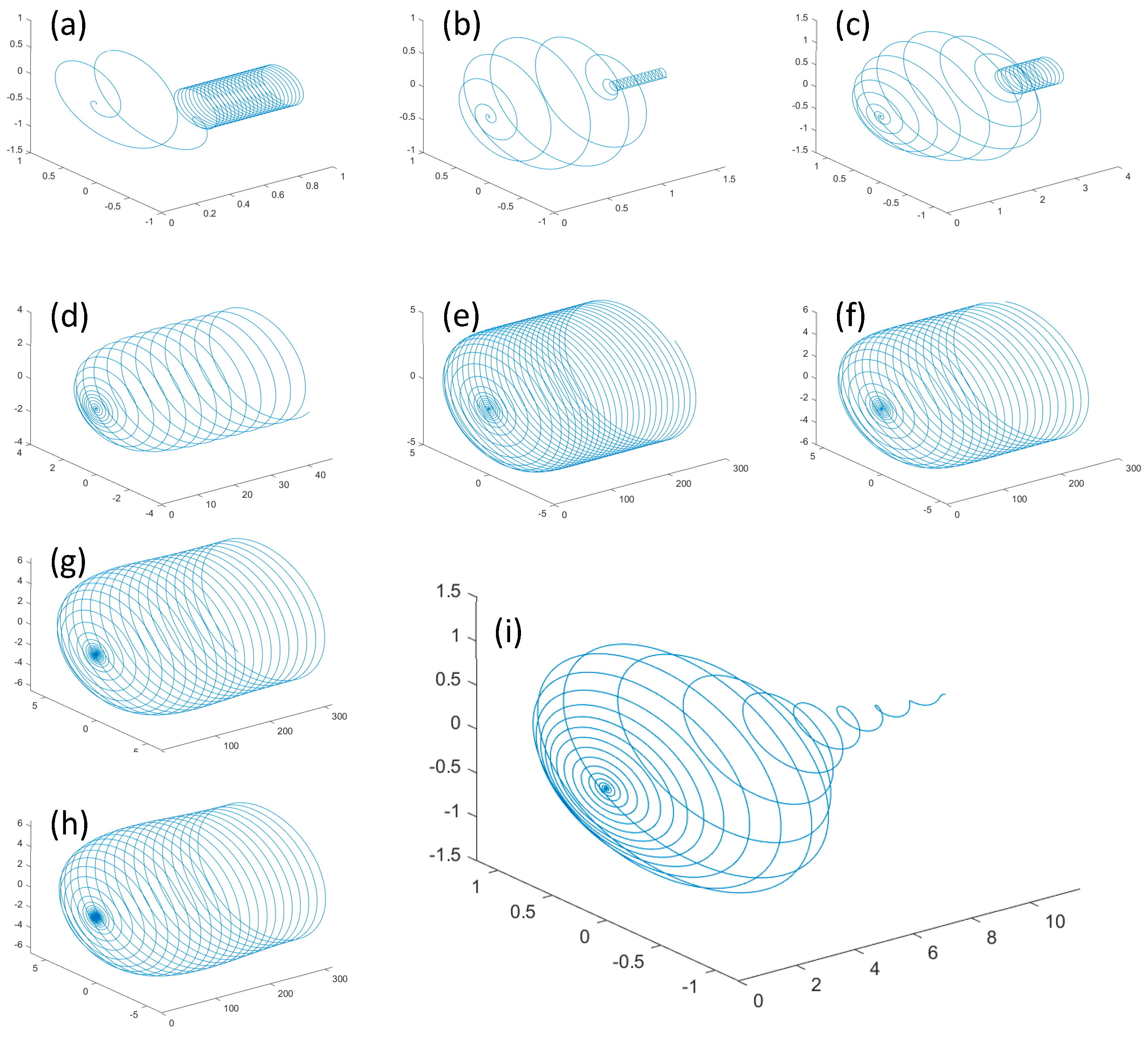
Figure 2 shows the trajectory of the electron at $\mathrm{L}=1{\mathsf{\lambda }}_0,\mathrm{L}=2{\mathsf{\lambda }}_0,\mathrm{L}=3{\mathsf{\lambda }}_0,\mathrm{L}=4{\mathsf{\lambda }}_0,\mathrm{L}=5{\mathsf{\lambda }}_0,\mathrm{L}=6{\mathsf{\lambda }}_0,\mathrm{L}=10{\mathsf{\lambda }}_0,\mathrm{L}=15{\mathsf{\lambda }}_0,\mathrm{B}=0.3$ under the combined effect of the laser pulse and magnetic field, and $\mathrm{L}=6{\mathsf{\lambda }}_0$ without the effect of the magnetic field.

The radial radii of the electron trajectories are 1, 1, 1.5, 4, 5, 5.5, 6,6, and 1.5, respectively in each image.

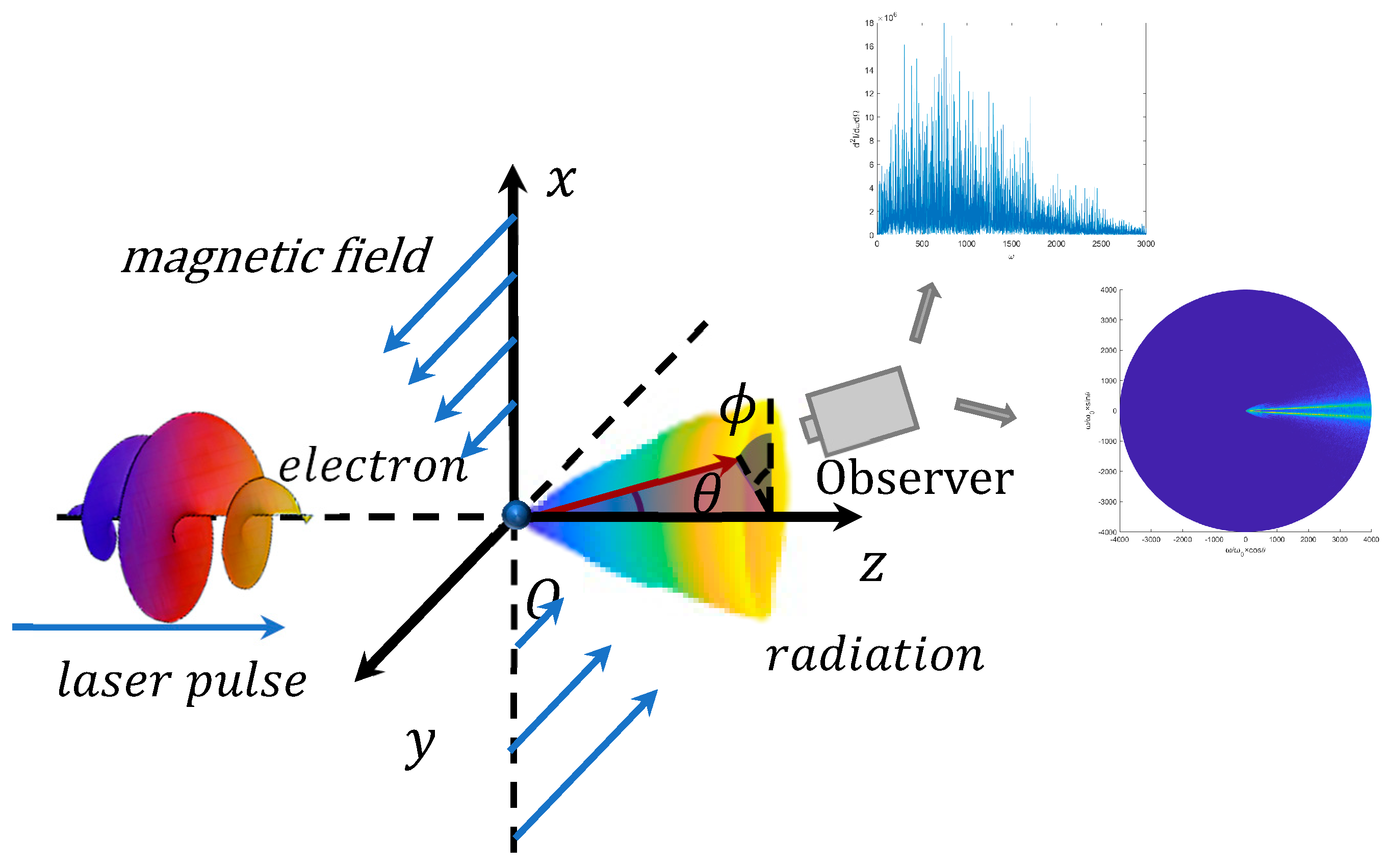
The axes labeled in the figure are the same as in the schematic; the direction of electron motion is the z-axis, the longitudinal axis is the x-axis, and the diagonal axis is the y-axis.

From Figure 2a–h, we can find that with laser and magnetic fields both acting, the electrons end up making a stable spiral motion with a specific amount of energy. When $\mathrm{L}={\mathsf{\lambda }}_0,2{\mathsf{\lambda }}_0,3{\mathsf{\lambda }}_0$, Figure 2a–c, the electron motion trajectory is a spiral that first becomes larger and then smaller, taking on an olive-like shape. Its final minimal value is a stable value. Specifically, the radial radii of the electrons are less than ${0.4\mathsf{\lambda }}_0$. This is due to the fact that the gradient between the rising and falling edges of the laser field is larger when the pulse width is smaller. As a result, the electron is subjected to significant acceleration and deceleration. The effect of deceleration on the electron is greater than the stabilizing effect of the magnetic field on the electron motion. Therefore, the electron in the smaller pulse width will appear in the first half of the olive-shaped and the second half of the spiral-shaped trajectory.

When $3{\mathsf{\lambda }}_0<\mathrm{L}<6{\mathsf{\lambda }}_0$, Figure 2d–h, the electron trajectory is a column-like helix, and its final value is a stable value. This is reflected in the increase of radial radius of the electron, which reaches saturation after $\mathrm{L}=6{\mathsf{\lambda }}_0$, and basically becomes stable at $6{\mathsf{\lambda }}_0$. This is due to the fact that the gradient between the rising and falling edges of the laser field is smaller at larger pulse widths. The acceleration and deceleration of the electrons are weaker. The effect of deceleration on the electrons is less than the stabilizing effect of the magnetic field on the electron motion. Therefore, the trajectory of the electron shows a stable spiral.

The radial maximum displacement also differs between the two. When $\mathrm{L}={\mathsf{\lambda }}_0,2{\mathsf{\lambda }}_0,3{\mathsf{\lambda }}_0,$ the radial maximum displacement of electrons is less than ${\mathsf{\lambda }}_0$, while after $\mathrm{L}>5{\mathsf{\lambda }}_0$, the radial maximum displacement of electrons increases with the increase of pulse width L, and both are greater than $5{\mathsf{\lambda }}_0$. This indicates that the magnetic field changes the trajectory of electron motion significantly.

This is due to the fact that when the pulse width is small, the gradient along the rise of the laser field is small and sweeps backward over the electron before the energy of the electron has been increased to a maximum, whereas when the pulse width is large, a sufficiently a long contact time is sufficient enough to maximize the energy of the electrons. When the pulse width continues to increase, the radial radius of the back end of the electron keeps getting larger and gradually remains constant because the gradient at the falling edge is smaller and the electron loses less energy due to the action of the magnetic field.

In addition, from Figure 2i, we can also see that the final energy of the electron without the magnetic field after the end of the laser field action is extremely small and close to a linear motion. Under the action of the laser field, the electron trajectory is helical with a maximum radial displacement less than ${\mathsf{\lambda }}_0$. The electron makes a nearly linear motion along the z-axis after about 10 Rayleigh lengths instead of a distinct helical forward motion.

The shape of the electron trajectory changes because the electrons remain in a stable spiral shape by the magnetic field even after the laser field action ends. When $\mathrm{L}>3{\mathsf{\lambda }}_0$, as the pulse width increases, the time of its influence becomes longer and the distance of the electron movement in the $\stackrel{⃑}{\mathrm{x}}$ and $\stackrel{⃑}{\mathrm{y}}$ directions increase.

Since the magnitude of the magnetic field is also influenced by the position in the x-direction, the radius of stable rotation of the final helix increases. The trajectory of the electrons then changes from the previous cut shape to a continuous column.

3.2. Space Radiation Characteristics of Electron

Figure 3 shows the spatial radiation map corresponding to the electron at $\mathrm{L}=1{\mathsf{\lambda }}_0,\mathrm{L}=2{\mathsf{\lambda }}_0,\mathrm{L}=3{\mathsf{\lambda }}_0,\mathrm{L}=4{\mathsf{\lambda }}_0,\mathrm{L}=5{\mathsf{\lambda }}_0,\mathrm{L}=6{\mathsf{\lambda }}_0,\mathrm{L}=10{\mathsf{\lambda }}_0,\mathrm{L}=15{\mathsf{\lambda }}_0,\mathrm{L}=6{\mathsf{\lambda }}_0,\mathrm{B}=0.3$ under the combined action of the laser pulse and the magnetic field, where the radiated power of the electron has been normalized by the maximum radiated power. The parameters of the laser are the same as above, and the initial state of the electron is stationary.

It can be seen from the figure that the radiation of electrons is concentrated in a narrow cone in the direction of motion of electrons (Z-axis), and the size of the angle between the central axis of the cone and the generatrix can be judged by the degree of energy concentration.

It is worth noting that the electron radiation power in Figure 3 is normalized by the maximum radiation power of the corresponding parameter itself. The specific values will be introduced in Section 3.3.

The maximum value of the color bar in the figure is 1, and the minimum value is 0.

We can find that the collimation of spatial radiation radiated by electrons without magnetic field is not strong and vortex-like. In contrast, the collimation of the energy radiated by electrons under the combined effect of laser and magnetic fields is significantly better.

Moreover, the collimation of electron radiation is slightly worse when $\mathrm{L}={\mathsf{\lambda }}_0,2{\mathsf{\lambda }}_0,3{\mathsf{\lambda }}_0$ under the combined effect of laser field and applied magnetic field. When $\mathrm{L}>3{\mathsf{\lambda }}_0$, the collimation of the electron radiation improves significantly, i.e., the angle between the central axis of the cone and the generatrix becomes smaller. We also find that when $\mathrm{L}>5{\mathsf{\lambda }}_0$, the collimation of the electron space radiation does not change much. There is a similarity with the electron motion trajectory shown in Figure 2.

However, we also find that as L increases, especially when $\mathrm{L}=10{\mathsf{\lambda }}_0,15{\mathsf{\lambda }}_0$ there appears an asymmetric in the radiation trajectory of the electrons, and in the positive direction of the z axes, we find less radiation from the electrons. Therefore, we consider the best outcome to be when $\mathrm{L}={6\mathsf{\lambda }}_0$.

Since the direction of radiation of an electron is the direction of the velocity of the electron’s motion [24]. Therefore, the greater the velocity of the electron in the z-axis direction compared to the velocity in the x-axis and y-axis directions, the better the collimation of the electron radiation. Whereas the intensity of electron radiated power is related to the velocity and acceleration of the electron, I will discuss the maximum electron radiated power intensity in Section 3.3.

The change of the shape and collimation of the electron space radiation is because when $\mathrm{L}={\mathsf{\lambda }}_0,2{\mathsf{\lambda }}_0,3{\mathsf{\lambda }}_0$ its electron trajectory is an unstable spiral combined with a stable spiral column. Therefore, its radiation is perturbed by the electron motion trajectory. As a result, the collimation is slightly poor. When $\mathrm{L}>4{\mathsf{\lambda }}_0$, the electron trajectory is a stable spiral column, the trajectory is stable, so the radiation collimation is better. In contrast, the electrons without magnetic field are not stable in their trajectory, so the collimation is worse than the electron radiation under the action of laser field and magnetic field.

3.3. Maximum Radiated Power Angle of Electrons and the Trend of Corresponding Radiated Power

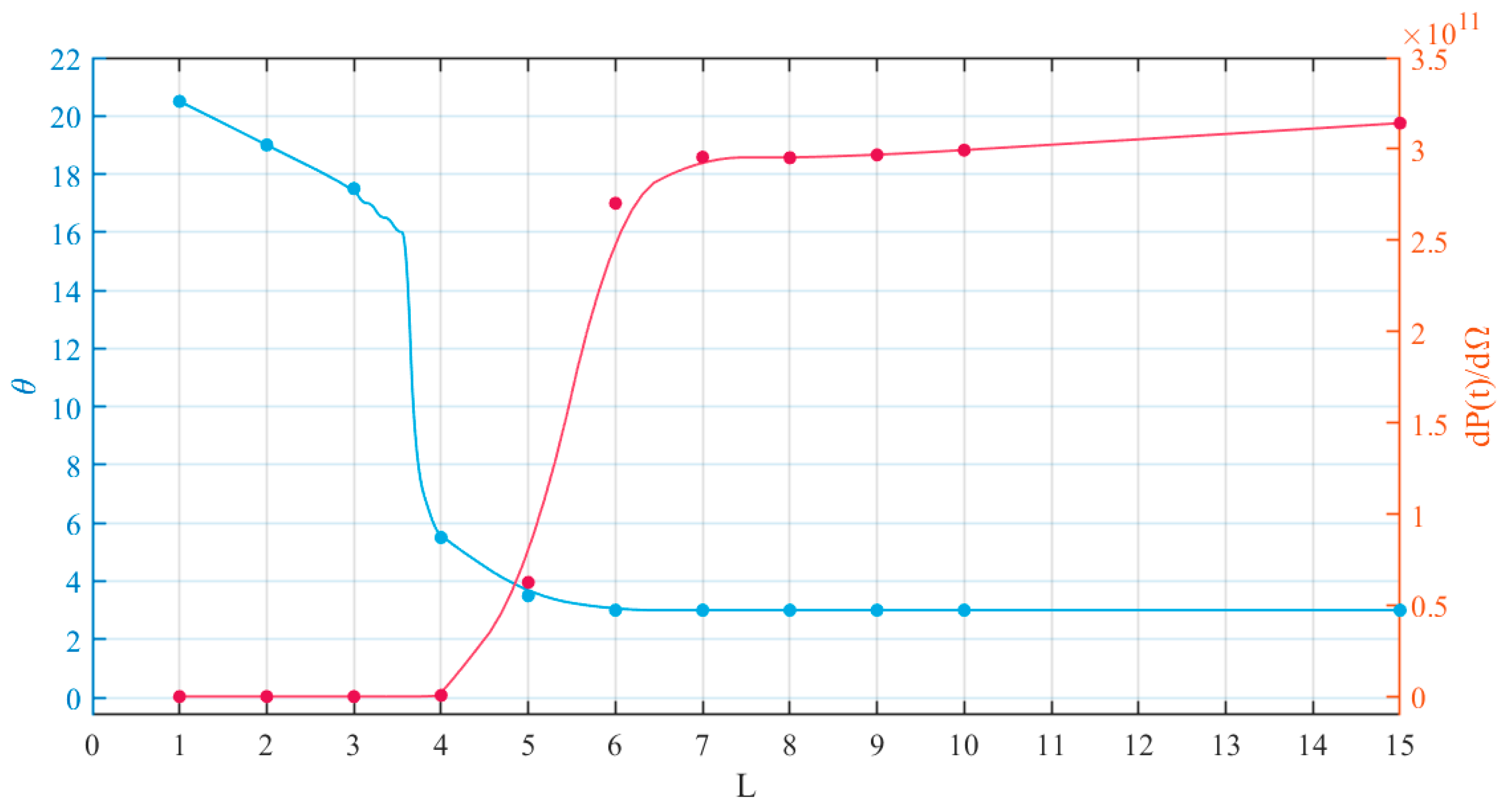
The blue line in Figure 4 is the maximum radiation power angle ${\mathsf{\theta }}_{\mathrm{m}\mathrm{a}\mathrm{x}}$ corresponding to the electron in the case of different pulse widths, and we can find its maximum radiation power angle decreases continuously when $\mathrm{L}<6{\mathsf{\lambda }}_0$, i.e., the collimation increases; and when $\mathrm{L}>6{\mathsf{\lambda }}_0$, it stabilizes at 3, i.e., it reaches the saturation state. Corresponding to the result of Figure 3, the change of collimation of radiation is reflected.

The red line in Figure 4 shows the radiated power corresponding to the maximum radiated power angle ${\mathsf{\theta }}_{\mathrm{m}\mathrm{a}\mathrm{x}}$ for electrons at different pulse widths. We can find that as the pulse width L increases, the corresponding radiated power tends to rise and reaches saturation roughly at $\mathrm{L}=6{\mathsf{\lambda }}_0$. This indicates that as the radiation collimation is enhanced, the power released from it also increases and finally reaches saturation at $\mathrm{L}=6{\mathsf{\lambda }}_0$. Corresponding to the result of Figure 3, the variation of the magnitude of the radiated power is reflected.

The reason why there is a situation such as the red line in the figure above is that when the pulse width L is small, the contact time between the laser field and the electrons is short, and the energy of the laser field can’t all be transferred to the electrons, so that the maximum radiated power of the electrons at the radiated power of the power is small. As the pulse width increases, the contact time between the laser field and the electrons becomes longer, and all the energy is transferred to the electrons, so the radiated power of the electrons reaches saturation.

3.4. Spectral Characteristics of Electron Radiation

Figure 5 shows the corresponding spectrum of electrons at the maximum radiation power angle ${(\mathsf{\theta }}_{\mathrm{m}\mathrm{a}\mathrm{x}},{\mathsf{\phi }}_{\mathrm{m}\mathrm{a}\mathrm{x}})$ with the same parameter settings as above. Figure 5a–h show the effect of laser pulses with different pulse widths on the higher harmonics of the electron radiation.

The maximum horizontal coordinates in the graph are: a, b: 1000; c, d: 1500; e, g, h: 200; f: 3000; i: 200.

The maximum vertical coordinates in the graph are: a: 1400; b: 7000; c: 12,000; d: 9 × 10⁵; e: 2.5 × 10⁶; g: 1.8 × 10⁷; h: 1.2 × 10⁶; f: 31.5 × 10⁶; i: 5000.

Firstly, observing Figure 5 from the perspective of the distribution of energy, we can easily see that for electrons in an applied magnetic field, its higher harmonics of the electron radiation reach a tenth of the peak energy at 500${\mathsf{\omega }}_0$ when the pulse width of the laser pulse is $\mathrm{L}={\mathsf{\lambda }}_0,2{\mathsf{\lambda }}_0,{3\mathsf{\lambda }}_0$. And as the pulse width of the laser pulse increases, the higher harmonics of the electron radiation increase. When $\mathrm{L}=4{\mathsf{\lambda }}_0$, the higher harmonics of the electron radiation reach a tenth of the peak energy at 800${\mathsf{\omega }}_0$.

When L > 6, the situation is similar to the one mentioned earlier, the electrons reach saturation, and the higher harmonics of the electron radiation are almost constant, both reaching a tenth of the peak energy at about 2000${\mathsf{\omega }}_0.$ However, the special point is that at $\mathrm{L}=6{\mathsf{\lambda }}_0$, the electron’s higher harmonics of the electron radiation do not reach a tenth of the peak energy until 2600 ${\mathsf{\omega }}_0$. This indicates that the electron’s high harmonics increase until saturation ($\mathrm{L}=6{\mathsf{\lambda }}_0$) under the combined effect of the tightly focused laser pulse and the magnetic field, and the best case is at $\mathrm{L}=6{\mathsf{\lambda }}_0$. We can assume that the tightly focused laser pulse with $\mathrm{L}=6{\mathsf{\lambda }}_0$ works best.

For the electron without the applied magnetic field, Figure 5i, its higher harmonics of the electron radiation reach a tenth of the peak energy at only 150${\mathsf{\omega }}_0$. This indicates the superiority of the method of modulating X-rays using an applied magnetic field compared to the conventional method, which has abilities that the conventional method does not have.

Furthermore, observing from the perspective of the distribution of energy magnitudes, we can find that the maximum energy of the electrons increases as the laser pulse L increases, from 1200 at $\mathrm{L}={\mathsf{\lambda }}_0$ to about 1.8 × 10⁷ at $\mathrm{L}={6\mathsf{\lambda }}_0$. However, when $\mathrm{L}={10\mathsf{\lambda }}_0,{15\mathsf{\lambda }}_0$, the higher harmonics of the electron radiation instead decrease to 1.1 × 10⁷ and 1.4 × 10⁷, respectively. This also corresponds to the conclusion above that tightly focused laser pulses at $\mathrm{L}={6\mathsf{\lambda }}_0$ work best.

It is due to the fact that as the spatial radiation collimation of electrons increases, at the maximum radiated power angle, we can observe more spectrums of electron radiation of different angles. While the spectrum on the maximum radiation power angle and the spectrum on the other azimuthal angles for superposition, resulting in higher harmonics of the electron radiation on the high ${\mathsf{\omega }}_0$ still have higher energy. That is to say, originally, the energy on different orientation has its fixed main frequency. When the spatial radiation collimation of electrons is improved, the spectrum on different orientation can be observed at the same time, forming the spectrum that can be observed in Figure 5a–h. Therefore, because of the asymmetry of the electrons in Figure 3 at pulse widths $\mathrm{L}=10{\mathsf{\lambda }}_0,15{\mathsf{\lambda }}_0$, the higher harmonic energy of the electrons is low and decreases quickly. Because the collimation of electrons in Figure 3 increases at pulse widths $\mathrm{L}={4\mathsf{\lambda }}_0~6{\mathsf{\lambda }}_0$, the higher harmonics of the electron radiation show approximately the same shape but with different magnitudes and distributions of energy. When $\mathrm{L}={\mathsf{\lambda }}_0~3{\mathsf{\lambda }}_0$, the electrons are less affected by the magnetic field, and the trajectory and spatial radiation of the electrons are approximately the same as the state without the magnetic field, so the shape of the spectrum does not change much [25], although the magnitude of the energy still has a significant increase.

3.5. Spectral Characteristics of Electron Radiation (2)

Figure 6 shows the spectrum of electrons under the influence of the corresponding radiated power angle $\mathsf{\theta }$ with the same parameter settings as above. Figure 6a–h show the effect of laser pulses with different pulse widths on the higher harmonics of the electron radiation and spatial distribution of the electrons.

The maximum vertical coordinates in the graph are: a, b, c, d, e, f, g, h: 3000; i: 1500.

Observing the figure from the perspective of energy distribution, it is easy to see that for electrons with an applied magnetic field, its spectrum becomes wider and wider when the pulse width of the laser pulse $\mathrm{L}={\mathsf{\lambda }}_0,2{\mathsf{\lambda }}_0,{3\mathsf{\lambda }}_0,{4\mathsf{\lambda }}_0,{5\mathsf{\lambda }}_0$. At the same time, the collimation of the spatial distribution increases, as the maximum energy also roughly reaches 1 × 10⁵. When $\mathrm{L}=6{\mathsf{\lambda }}_0,10{\mathsf{\lambda }}_0,{15\mathsf{\lambda }}_0$, the spatial distribution collimation of electrons decreases. However, the distribution of its higher harmonics of the electron radiation is different. For example, when $\mathrm{L}=6{\mathsf{\lambda }}_0$, although its radiated power angle at the maximum of the highest harmonic, i.e., the maximum radiated power angle ${\mathsf{\theta }}_{\mathrm{m}\mathrm{a}\mathrm{x}}$ is small, but the radiated power angle at the lower of the higher harmonic still has about 18°. While $\mathrm{L}=15{\mathsf{\lambda }}_0$, there is no such problem; the radiation power angle and the maximum radiation power angle are almost the same. That is, there are no some smaller interference sources.

However, when observing Figure 6i, we find that the higher harmonics of the electron radiation are extremely small, the energy is also extremely low, and the spatial collimation is extremely poor. This also reflects the superiority of the X-ray modulation method by an applied magnetic field.

4. Conclusions

From the perspective of electron dynamics analysis, electrons in the smaller pulse width of the impact of the trajectory are relatively small because of the smaller role of the magnetic field, so the trajectory for the larger and then the smaller spiral is finally stabilized at a stable value. The larger pulse width tends to stabilize the spiral column. The spatial radiation properties of the electron also correspond to the trajectory of the electron. Collimation is poor at smaller pulse widths, while as the pulse width increases, the maximum radiated power angle stabilizes and collimation becomes better. When the pulse width is greater than 6${\mathsf{\lambda }}_0$, the spatial radiation of the electrons appears to be asymmetric. The spectral characteristics of the electron radiation are also roughly the same as the first two characteristics and are optimal when the pulse width is equal to 6${\mathsf{\lambda }}_0$. When the pulse width is small, there is less influence of the magnetic field, and the spectrum is approximately the same as that without the magnetic field, while its repeatability increases as the pulse width increases due to the predominance of the magnetic field and less influence of the tightly focused laser field. The maximum value of the spectral energy is greatest when the pulse width is equal to 6${\mathsf{\lambda }}_0$ because the collimation is best and the corresponding radiation is available in all directions. When the pulse width is greater than 6${\mathsf{\lambda }}_0$, the asymmetry increases and the maximum value of the corresponding spectral energy decreases more quickly.

Therefore, in order to obtain high-energy, highly collimated X-rays with a given laser pulse beam radius and peak laser amplitude, modulation can be performed by applying a magnetic field and increasing the pulse width. The resulting X-rays not only increase tremendously in energy but also become highly collimated. However, it should be noted that although the collimation of the radiation and the magnitude of the radiated power are optimal at a pulse width of 6${\mathsf{\lambda }}_0$, some small sources of interference can be found in the X-rays corresponding to $\mathrm{L}=6{\mathsf{\lambda }}_0$ in Figure 6.This leads to the fact that although the maximum power angle of the X-rays at $\mathrm{L}=6{\mathsf{\lambda }}_0$ is extremely small, the actual maximum value of θ is still not the minimum. Therefore, if we need X-rays with excellent collimation, it is better to use X-rays with a pulse width $\mathrm{L}=15{\mathsf{\lambda }}_0$ modulation. The maximum value of the corresponding spatial power angle at this point is the smallest, i.e., the best collimation.

This gives us a good way to use nonlinear Thomson scattering for scientific experiments and some potential applications of modulated X-rays.

References

1. Strickland, D.; Mourou, G. Compression of amplified chirped optical pulses. Opt. Commun. 1985, 55, 447–449. [Google Scholar] [CrossRef]
2. Eidam, T.; Hanf, S.; Seise, E.; Andersen, T.V.; Gabler, T.; Wirth, C.; Schreiber, T.; Limpert, J.; Tünnermann, A. Femtosecond fiber CPA system emitting 830 W average output power. Opt. Lett. 2010, 35, 94–96. [Google Scholar] [CrossRef] [PubMed]
3. Beiersdorfer, P. Laboratory X-Ray Astrophysics. Annu. Rev. Astron. Astrophys. 2003, 41, 343–390. [Google Scholar] [CrossRef]
4. Taira, Y.; Hayakawa, T.; Katoh, M. Gamma-ray vortices from nonlinear inverse Thomson scattering of circularly polarized light. Sci. Rep. 2017, 7, 5018. [Google Scholar] [CrossRef]
5. Salamin, Y.I.; Harman, Z.; Keitel, C.H. Direct High-Power Laser Acceleration of Ions for Medical Applications. Phys. Rev. Lett. 2008, 100, 155004. [Google Scholar] [CrossRef] [PubMed]
6. Lan, P.; Lu, P.; Cao, W.; Li, Y.; Wang, X. Carrier-envelope phase-stabilized attosecond pulses from asymmetric molecules. Phys. Rev. A 2007, 76, 021801. [Google Scholar] [CrossRef]
7. Chi, Z.; Du, Y.; Huang, W.; Tang, C. Linearly polarized X-ray fluorescence computed tomography based on a Thomson scattering light source: A Monte Carlo study. J. Synchrotron Radiat. 2020, 27, 737–745. [Google Scholar] [CrossRef]
8. Lee, K.; Chung, S.Y.; Park, S.H.; Jeong, Y.U.; Kim, D. Effects of high-order fields of a tightly focused laser pulse on relativistic nonlinear Thomson scattered radiation by a relativistic electron. EPL Europhys. Lett. 2010, 89, 64006. [Google Scholar] [CrossRef]
9. Baltuška, A.; Udem, T.; Uiberacker, M.; Hentschel, M.; Goulielmakis, E.; Gohle, C.; Holzwarth, R.; Yakovlev, V.S.; Scrinzi, A.; Hänsch, T.W.; et al. Attosecond control of electronic processes by intense light fields. Nature 2003, 421, 611–615. [Google Scholar] [CrossRef]
10. Salamin, Y.I.; Faisal, F.H.M. Relativistic free-electron dynamics and light-emission spectra in the simultaneous presence of a superintense laser field and a strong uniform magnetic field. Phys. Rev. A 1998, 58, 3221–3234. [Google Scholar] [CrossRef]
11. Faisal, F.H.M.; Salamin, Y.I. Electron dynamics and photon-emission spectra in an ultrashort laser pulse and a uniform magnetic field. Phys. Rev. A 1999, 60, 2505–2516. [Google Scholar] [CrossRef]
12. Salamin, Y.I.; Faisal, F.H.M.; Keitel, C.H. Exact analysis of ultrahigh laser-induced acceleration of electrons by cyclotron autoresonance. Phys. Rev. A 2000, 62, 053809. [Google Scholar] [CrossRef]
13. Yu, W.; Bychenkov, V.; Sentoku, Y.; Yu, M.Y.; Sheng, Z.M.; Mima, K. Electron Acceleration by a Short Relativistic Laser Pulse at the Front of Solid Targets. Phys. Rev. Lett. 2000, 85, 570–573. [Google Scholar] [CrossRef] [PubMed]
14. Yu, W.; Chen, Z.Y.; Yu, M.Y.; Qian, L.J.; Lu, P.X.; Li, R.X.; Koyama, K. Electron acceleration and high-order harmonic generation by an intense short pulse laser in a magnetic field. Phys. Rev. E 2002, 66, 036406. [Google Scholar] [CrossRef] [PubMed]
15. Gong, J.X.; Cao, L.H.; Pan, K.Q.; Xiao, C.Z.; Wu, D.; He, X.T. Enhancing the electron acceleration by a circularly polarized laser interaction with a cone-target with an external longitudinal magnetic field. Phys. Plasmas 2017, 24, 033103. [Google Scholar] [CrossRef]
16. Ghotra, H.S.; Kant, N. Polarization effect of a Gaussian laser pulse on magnetic field influenced electron acceleration in vacuum. Opt. Commun. 2016, 365, 231–236. [Google Scholar] [CrossRef]
17. Zhao, L.; Chen, Z.-J.; Sang, H.-B.; Xie, B.-S. Spatial Characteristics of Thomson Scattering Spectra in Laser and Magnetic Fields. Chin. Phys. Lett. 2019, 36, 074101. [Google Scholar] [CrossRef]
18. Wang, Y.; Zhou, Q.; Zhuang, J.; Yu, P.; Tian, Y. Vortex and symmetric radiation character of nonlinear Thomson scattering in Laguerre-Gaussian circularly polarized laser pulses. Opt. Express 2021, 29, 22636–22647. [Google Scholar] [CrossRef]
19. Li, K.; Li, L.; Shu, Q.; Tian, Y.; Shi, Y.; Zhang, Z. Spatial characteristics of motion and emission from electron driven by linearly polarized tightly focused laser pulses. Optik 2019, 183, 813–817. [Google Scholar] [CrossRef]
20. Wang, Y.; Wang, C.; Li, K.; Li, L.; Tian, Y. Spatial radiation features of Thomson scattering from electron in circularly polarized tightly focused laser beams. Laser Phys. Lett. 2020, 18, 015303. [Google Scholar] [CrossRef]
21. Yan, Y.L.; Zhou, X.; Ren, S.L.; Liu, H.; Tian, Y.W. Influence of electron’s initial position on spatial radiation of high-energy electrons. Laser Technol. 2022, 46, 556. [Google Scholar] [CrossRef]
22. Yu, P.; Lin, H.; Gu, Z.; Li, K.; Tian, Y. Analysis of the beam waist on spatial emission characteristics from an electron driven by intense linearly polarized laser pulses. Laser Phys. 2020, 30, 045301. [Google Scholar] [CrossRef]
23. Wu, Y.; Liu, Y.; Liu, D.; Tian, Y. Effect of circularly polarized laser pulse beam waist radius on the dynamic and radiation characteristics of collided electrons. Laser Phys. 2020, 30, 115301. [Google Scholar] [CrossRef]
24. Corde, S.; Phuoc, K.T.; Lambert, G.; Fitour, R.; Malka, V.; Rousse, A.; Beck, A.; Lefebvre, E. Femtosecond x rays from laser-plasma accelerators. Rev. Mod. Phys. 2013, 85, 1. [Google Scholar] [CrossRef]
25. Wang, H.L.; Xia, F.Y.; Tian, Y.W. Simulation calculation of the influence of pulse width on the peak radiation of laser impact electron. Laser Technol. 2020, 46, 561. [Google Scholar] [CrossRef]
Figure 1. The schematic diagram of nonlinear Thomson scattering.
Applsci 13 11710 g001
Figure 2. Trajectory diagram of the electron (a) L = λ 0 , B = 0.3, (b) L = 2 λ 0 , B = 0.3, (c) L = 3 λ 0 , B = 0.3, (d) L = 4 λ 0 , B = 0.3, (e) L = 5 λ 0 , B = 0.3, (f) L = 6 λ 0 , B = 0.3, (g) L = 10 λ 0 , B = 0.3, (h) L = 15 λ 0 , B = 0.3, (i) L = 6 λ 0 , B = 0.
Applsci 13 11710 g002
Figure 3. Space radiation diagram of electrons (a) L = λ 0 , B = 0.3, (b) L = 2 λ 0 , B = 0.3, (c) L = 3 λ 0 , B = 0.3, (d) L = 4 λ 0 , B = 0.3, (e) L = 5 λ 0 , B = 0.3, (f) L = 6 λ 0 , B = 0.3, (g) L = 10 λ 0 , B = 0.3, (h) L = 15 λ 0 , B = 0.3, (i) L = 6 λ 0 , B = 0.
Applsci 13 11710 g003
Figure 4. Maximum radiated power angle of electrons (blue) and the trend of corresponding radiated power (red).
Applsci 13 11710 g004
Figure 5. Spectral characteristics of electron radiation (a) L = λ 0 , B = 0.3, (b) L = 2 λ 0 , B = 0.3, (c) L = 3 λ 0 , B = 0.3, (d) L = 4 λ 0 , B = 0.3, (e) L = 5 λ 0 , B = 0.3, (f) L = 6 λ 0 , B = 0.3, (g) L = 10 λ 0 , B = 0.3, (h) L = 15 λ 0 , B = 0.3, (i) L = 6 λ 0 , B = 0.
Applsci 13 11710 g005
Figure 6. Spectrogram of electrons under the influence of the corresponding radiated power angle (a) L = λ 0 , B = 0.3, (b) L = 2 λ 0 , B = 0.3, (c) L = 3 λ 0 , B = 0.3, (d) L = 4 λ 0 , B = 0.3, (e) L = 5 λ 0 , B = 0.3, (f) L = 6 λ 0 , B = 0.3, (g) L = 10 λ 0 , B = 0.3, (h) L = 15 λ 0 , B = 0.3, (i) L = 6 λ 0 , B = 0.
Applsci 13 11710 g006
Disclaimer/Publisher’s Note: The statements, opinions and data contained in all publications are solely those of the individual author(s) and contributor(s) and not of MDPI and/or the editor(s). MDPI and/or the editor(s) disclaim responsibility for any injury to people or property resulting from any ideas, methods, instructions or products referred to in the content.