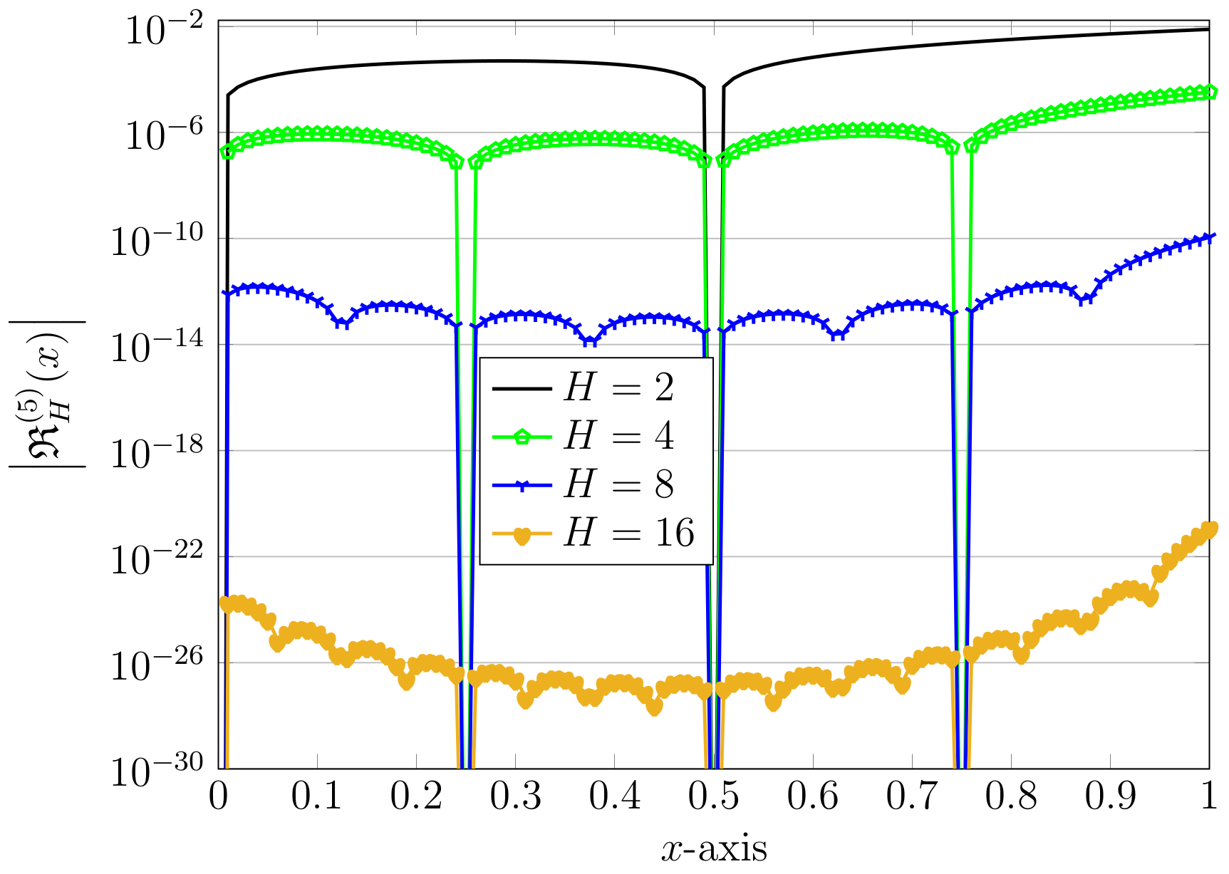
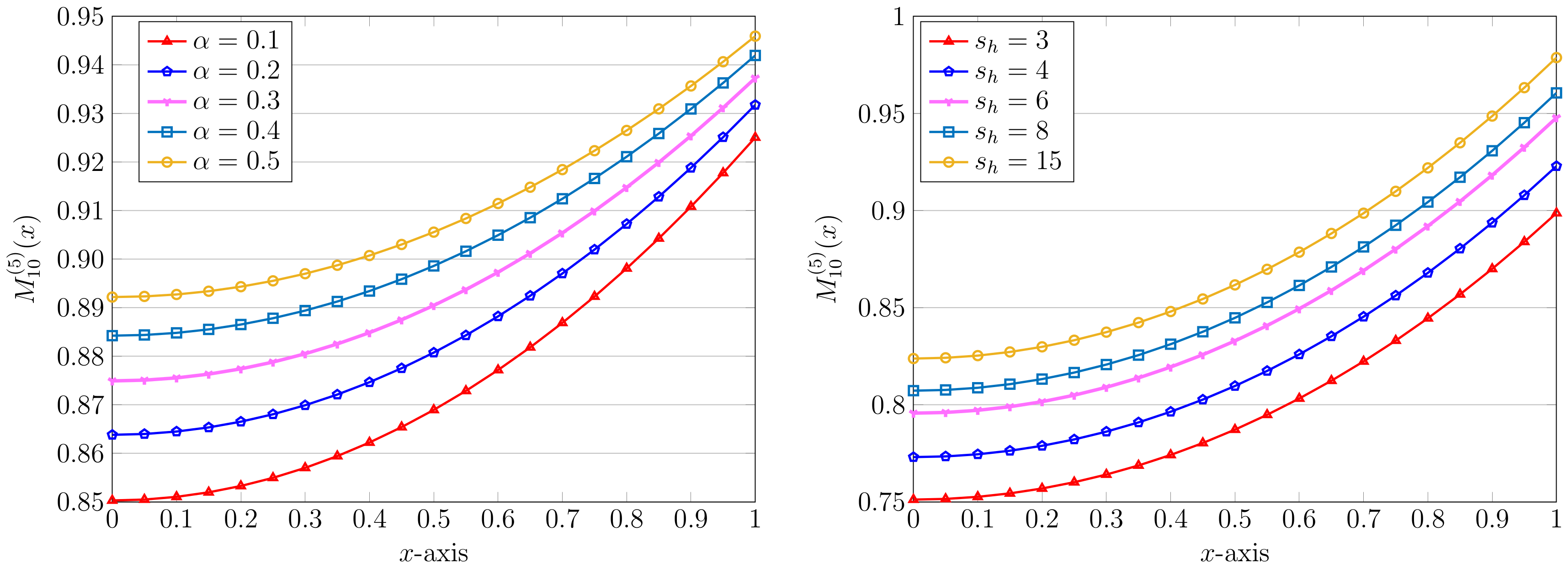
Abstract
A hybrid efficient and highly accurate spectral matrix technique is adapted for numerical treatments of a class of two-pint boundary value problems (BVPs) with singularity and strong nonlinearity. The underlying model is a reaction-diffusion equation arising in the modeling of biomedical, chemical, and physical applications based on the assumptions of Michaelis–Menten kinetics for enzymatic reactions. The manuscript presents a highly computational spectral collocation algorithm for the model combined with the quasilinearization method (QLM) to make the proposed technique more efficient than the corresponding direct spectral collocation algorithm. A novel class of polynomials introduced by S.K. Chatterjea is used in the spectral method. A detailed proof of the convergence analysis of the Chatterjea polynomials (ChPs) is given in the norm. Different numerical examples for substrate concentrations with all values of parameters are performed for the case of planar and spherical shapes of enzymes. For validation, these results are compared with those obtained via wavelet-based procedures and the Adomian decomposition scheme. To further improve the approximate solutions obtained by the QLM–ChPs method, the technique of error correction is introduced and applied based on the concept of residual error function. Overall, the presented results with exponential convergence indicate that the QLM–ChPs algorithm is simple and flexible enough to be applicable in solving many similar problems in science and engineering.
1. Introduction
An enzyme is a substance produced by a living organism, which acts as a catalyst to bring about a specific biochemical reaction. In other words, enzymes are proteins that help speed up metabolism or the chemical reactions in our bodies. They build some substances and break others down. Every living creature has enzymes, and our bodies naturally produce enzymes. Biosensors are analytical devices consisting of a biological entity, typically an enzyme, that recognizes a specific analyte and a transducer that transforms biomolecules into an electric signal [1]. These instruments have been widely utilized in environmental, medical, and industrial applications due to their high selectivity, simplicity, and low cost [2]. Using a mathematical model that is based on reaction–diffusion (RD) equations would be a useful tool for studying the performance of biosensors of any kind [3]. This class of (steady-state) RD equations has a nonlinear term that is associated with the so-called Michaelis–Menten kinetics of the enzymatic reaction [4]. Several processes in the physical, biological, and chemical sciences can be described in terms of the Michaelis–Menten (MM) kinetics model. Among others, we emphasize the mathematical model for oxygen diffusion in a spherical cell using the MM oxygen uptake kinetics proposed and solved in [5]. Later, this model was resolved and re-examined in [6]. A study of the steady-state substrate concentration in the action of biosensor response at mixed enzyme kinetics was investigated in [7]. A mathematical model relying on catechol–polyphenol oxidase as a prototype electroenzymatic model system was given in [8]. The cubic-autocatalysis with MM kinetics in a 1D RD cell was examined in [9].
Let us consider the MM reaction scheme, which has been utilized to analyze bulk experiments. In accordance with the assumptions of the model, an enzyme binds a substrate in a reversible manner to constitute an enzyme–substrate complex . Then, a conversion of the substrate can be done to either a product by the enzyme or alternatively unbind. The process of enzymatic catalysis is subsequently used to dissociate into and . Schematically, the MM process can be described as follows:
Here, the two constants and represent the rates at which the forward and reverse process reacted, respectively. Additionally, the constant indicates the catalysis rate of the subsequent process. For the above system, the following nonlinear MM equation is held as
where denotes the concentration of the substrate , the maximum velocity of the system is shown by , and stands for the substrate concentration at which the velocity of the reaction is fifty percent of .
By introducing the following non-dimensional parameters (see Table 1 for the parameters’ definitions) [10]
we arrive at the (non-dimensional) material balance of substrate species inside the support. Mathematically, it can be formulated as follows [10,11]:
Here, the component n describes the shape of the immobilized catalyst. For , the shape is a slab, while for , we have a spherical shape. The prescribed boundary conditions of the former model Equation (1) can be given as
Here, the parameter represents a modified Sherwood number and is defined as . Additionally, shows the mass-transfer coefficient.

Table 1.
Nomenclature.
It can be clearly seen that the mathematical modeling of the above-mentioned system led to a two-point boundary value problem (BVP) with a strong nonlinearity term. This model will also be singular for . These facts make it difficult to predict the behavior of the system by solving the BVP (1)–(2) analytically. Thus, the numerical and approximation algorithms have preferably been proposed in practice. In this respect, the integral equation method was considered in [12] to deal with (1). The Runge–Kutta method of order four together with the bisection methods were utilized in [5] and re-examined in [6] later. Two semi-analytical approaches, i.e., the homotopy perturbation and He’s variational iteration schemes presented in [7] were used to solve a variant of (1). The Maclaurin series solution in the case of a spherical cell was investigated in [13]. The Adomian decomposition method (ADM) was developed in [10] to find an analytical solution to the model in [10]. Recently, in [11], the authors proposed a wavelet technique based on the Chebyshev and Legendre bases to solve the above BVP. A similar method based on the ultra-spherical wavelet was examined in [14]. The optimal homotopy analysis procedure was applied to the model (1) in [15]. The technique of the B-Spline collocation scheme was employed in [16]. A hybrid method based on the modified ADM and quintic B-spline collocation strategy was given in [17]. Moreover, the shifted Chebyshev collocation procedure for the spherical biocatalyst and catalyst models was investigated in [18]. Some other numerical methods developed for the model (1) and the models close to it can be found in [19,20,21,22].
Our purpose here is to propose a new strategy to solve the strongly nonlinear model (1) efficiently and accurately. The present algorithm is based on a combination of the quasilinearization method (QLM) and the spectral collocation approach for the nonlinear model (1). The technique of QLM is first employed to eliminate both the nonlinearity and singularity of the underlying model. The result is a sequence of linearized submodels that have to be solved iteratively. In the second stage, we develop a matrix method based on the (novel) class of polynomials along with certain collocation points to acquire the approximate solutions of this set of linearized equations. This new class of polynomials is very closely related to the Bessel function of Krall and Frink. We further establish the convergence property of these polynomials in the norm. The technique of residual correction is also introduced to improve the accuracy of the already-computed solutions and based on the residual error functions. Over the last decade, thanks to the successful applications of spectral and collocation methods based on (various) polynomial functions, rapid progress has been made towards solving many interesting and challenging model problems in physical and engineering sciences. Among the multitude of used basis functions, we mention the Bessel [23], Laguerre [24], Jacobi [25,26], Chebyshev [27], Newton [28], Fibonacci [29], and Morgan-Voyce [30,31] polynomials.
Let us describe the content of this research paper in more detail as follows. A review of main facts associated with this new class of polynomials known as the Chatterjea polynomials (ChPs) is provided in Section 2. In Section 3, we first illustrate the main idea of QLM. Hence, the hybrid QLM–ChPs algorithm is described in detail. The error bound for the proposed QLM–ChPs scheme is investigated next. The accuracy of the present approach is justified by defining the technique of residual error functions. Finally, in this section, we introduce the technique of residual correction (RC), which helps us to improve the quality of the approximate solutions. We next carry out a set of computational experiments to analyze the computational efficiency as well as the accuracy of the QLM–ChPs procedure for the considered model problem in Section 4. Ultimately, in Section 5, we present the conclusions of the current work.
2. A Review of a New Class of Polynomials
In this part, we consider a new class of polynomials related to the simple Bessel polynomials of Krall–Frink [32]. This class of polynomials was investigated by S.K. Chatterjea in [33]. This set is closely connected to Rodrigues’ formula for a positive integer h. In addition to this variant class of polynomials, different usages of Krall–Frink Bessel polynomials have been successfully shown in the literature to solve integer as well as fractional order differential equations; see for instances [34,35,36] and the recently reviewed paper [37] for the complete biography. Below, we recall some basic facts associated with the Chatterjea polynomials, and for more details, refer to [33].
2.1. The Chatterjea Polynomials
Let us first denote the Chatterjea polynomials (ChPs) of order h by . In Rodrigues’ format, the ChPs are defined by
On the other hand, they can be represented by the hypergeometric functions as
Some mathematical connections between this class of polynomials and the Laguerre and Bessel polynomials were also proved, as mentioned above. However, we are interested in the explicit form of ChPs. It is as follows
According to the former formula, we easily find that . The list of the next five ChPs is given for the convenience of reference as
Clearly, we have for all . Additionally, note that the coefficients of all ChPs are positive. The next result indicates that these ChPs are the solutions of a differential equation of the second order given by
Finally, we derive a decomposition for the vector of ChPs basis functions that will be utilized below. In this respect, we set
where H is a given integer. In terms of monomial bases, we obtain the next result.
Lemma 1.
Proof.
The proof is an easy exercise. □
2.2. Convergent of ChPs in the Sense of
Here, we establish a convergence result, which validates the proposed collocation matrix approach from the theoretical point of view. Every function that a square-integrable function on may be expanded as a sum of functions. To proceed, we set , which is a Hilbert space. Thus, for , we have
The task is here to find the unknown coefficients for . To deal with the underlying model (1), we need to take a finite number of bases in (7). In this work, we use only terms of the aforementioned infinite series. By cutting it, we obtain
Here, the vector of basis functions, i.e., , is previously defined in (5). The other object is the vector of unknowns represented by
Our ultimate goal is to measure the difference between and in the norm, in particular, as H tends to infinity. Based on the above arguments, we now constitute a finite-dimensional space as a subspace of . It is defined by
It can be clearly seen that , which means that is a closed subset of V and therefore constitutes a complete subspace of V. The immediate conclusion is that for an arbitrary element , we can find a closest approximation from . Let us denote this best approximation by . Mathematically speaking, we have
Here, and .
Let us state and prove the following theorem regarding the quality of the approximate solution for the function .
Theorem 1.
If is -times a continuously differentiable function on and if represents the closest unique approximation to in the space , then the following error bound is valid
where in the error term of approximation.
Proof.
We let be an arbitrary (but fixed) point in . By employing the Taylor series expansion of near the point , we obtain
where lies between and . Here, denotes the remainder term of the Taylor formula, for which we have
Under the assumption of the theorem, we know that stands for the closest best approximation to . It follows that
By replacing in the foregoing inequality by the Taylor approximation , we conclude that
On accounting the upper bound for the remainder of the Taylor formula given in (10), we have
By calculating the integral term, we arrive at
where .
We claim that . One can easily check that and for all . Therefore, the maximum absolute value of f will be attained at either the endpoint or . In both cases, we have . The proof is now concluded by taking the square roots of the former inequality. □
It should be remarked that by letting , the error norm converges to 0.
3. Description of QLM–ChPs Matrix Approach
The chief goal of the current work is to devise an efficient as well as accurate matrix algorithm based on the ChPs described above. Towards this end, we first rewrite the original nonlinear model problem (1) in the form
As mentioned before, we are particularly interested in and . Obviously, the model under consideration is not only strongly nonlinear but also singular at the origin. Of course, when , the second term is annihilated. These hinder us to solve the model problem efficiently and accurately. In particular, by applying the direct collocation matrix techniques using the (finite) expansion series (8), we arrive at an algebraic nonlinear system of equations of size . To obtain high-order accuracy, one has to increase H. In this case, the target nonlinear solvers (such as the Newton–Raphson algorithm) are usually unsuccessful in returning the right solutions.
In order to have no such difficulty, one remedy is to linearize the model (11) first. The Bellman’s quasilinearization method (QLM) can be used for this purpose. Thus, we have to solve a sequence of linearized submodels rather than a single nonlinear model. The wide range of applicability of the QLM to diverse initial and boundary value problems has been shown by many researchers; we refer for comparison [38,39,40].
3.1. The Essence of QLM
The nonlinear model (11) can be further reformulated in a concise format as
where
Note that the boundary conditions (2) are also given with (12). To begin with QLM, we are required to set an initial guess as an approximation for the true solution of (12). Hence, the QLM for the model Equation (12) is written generally as
for . Here, the represents the derivative of with regard to M. The same is valid for . Making use of QLM for the model (12) gives us
In order to write the former equations in a more convenient format, we multiply both sides by . By introducing the notations
we arrive at the next set of linearized equations
The boundary conditions (2) are now converted to the following forms
Now, the task is to solve the family of boundary value problems (13) and (14). This can now be accomplished by using the direct spectral collocation approach based on ChPs.
3.2. The Main Algorithm
To approximate the solutions of the linearized boundary value problems (13) and (14) via the QLM–ChPs technique, we assume that we have the approximation at hand for the solution of (13) at the iteration . In the next iteration, we take
where contains the vector of unknowns at the iteration number . We also recall that the vector as well as the matrix are previously introduced in (5) and (6). We, moreover, need a set of collocation nodes on . By uniform partitioning of this interval, we set these points as
By collocating the approximate solution in (15) at the points (16), we obtain the next matrix format
where we have
In the next stage, we need to compute the first and second derivatives of in (15). A straightforward computation reveals that
To calculate the derivative of , we note that
By combining two preceding relations, we arrive at
Similarly, by repeating the differentiation once more, we obtain the next representation
To show the first and second derivatives of in (18) and (19) in a matrix representation form, we state the next lemma.
Lemma 2.
Proof.
In the next step of our algorithm, we return to the linearized equations (13) and put the collocation nodes into them to obtain
for and . We are able to rewrite the former equations (21) compactly by the aid of the following notations
The resultant system of equations is shown by
The next fundamental matrix of the equation is derived by employing the foregoing relations (17)–(20) for the vectors , , and in (22). It follows that
where for .
By solving the above fundamental matrix Equation (23), we obtain a solution for the linearized Equation (13). However, this solution needs to be satisfied in the boundary conditions (14). So, in the final stage, we derive the matrix formats for the boundary conditions. For the first Neumann boundary condition, we utilize the relation (18). It is sufficient to tend . This gives us
For the second mixed boundary condition (14), we use a combination of two relations, (15) and (18). Here, we need to tend . We can now reformulate the second boundary condition in the form of a matrix given by
By returning to the augmented matrix , we now replace the first and last row of it with the new rows and obtained in (24) and (25), respectively. By updating the former fundamental matrix Equation (23), we arrive at the new modified version denoted by
Any linear solver can be utilized to solve the system (26). Therefore, after knowing the coefficients at iteration e, , we obtain the approximate solution of the strongly nonlinear model (1) on . The utility of the proposed QLM–ChPs algorithm will be considered in the next section.
3.3. Theoretical Upper Bound for QLM–ChPs Approach
In Theorem 1, we have obtained an upper bound for the error between as the true solution of the original model problem (1) and its approximation expanded in terms of ChPs in (8). This error is defined by
Our aim is now to examine the error between and as the approximate solution of the associated linearized model problem (13) together with boundary conditions (14) at a fixed iteration number e. Let this error be represented by and defined by
The next theorem consists of an error estimate for the QLM–ChPs solution.
Theorem 2.
Let the assumptions of Theorem 1 hold. Then, the upper bound for the error is given by
Proof.
Our proof starts with the following error decomposition
where denotes the difference between the approximate solutions of (13) and (1) when solving with the ChPs collocation procedures. One can immediately write the following conclusion using the triangle inequality
For the first term, we apply the result of Theorem 1, which asserted that
We now need to obtain an upper bound for the second term . We recall that the approximate solutions and can be stated as
in accordance to relations (8) and (15), respectively. Here, we have the corresponding coefficients obtained by the direct ChPs and QLM–ChPs collocation matrix procedures as
The consequence is that
For the first term, we further have
By comparing to the corresponding harmonic series, we can find that , where is the Euler constant. Now, by inserting the upper bounds for and in the inequity (30), we have completed the proof. □
It seems that the obtained upper bound for the error term is not sufficiently small in practical problems. However, we will show that this upper bound is quite tight when computed for the actual experimental results.
3.4. Error Measurement via REF Method
Due to the existence of the strongly nonlinear term in the reaction–diffusion model (1), finding exact true solutions is out of reach. This is the main reason why devising numerical methods is important for this model. However, to check how the proposed approach approximates the solutions of this model, we require having some tools for computing the achieved errors. One approach is based on the residual error functions (REFs) technique. The REFs can be obtained by putting the obtained approximate solution into the original differential model (1). Concisely speaking, we set the REFs for our model problem as
In an equivalent form, we may write the REFs in the form
We note that when , the former REFs reduces to the following form
3.5. The RC Methodology
In this part, we concentrate on the linearized boundary value problems (BVPs) (13) and (14). We first define the associated residual function of the linear operators. We then correct the current approximated solution by the technique of residual correction (RC). To do so, we first fix the iteration e and rewrite the BVPs (13) as
where is a linear differential operator. We also define the error term
where is the exact solution of (34), and shows the approximate solution obtained by the QLM–ChPs approach as given in (15). The associated residual function is defined by
It is evident that we have
We now arrive at the error problem by subtracting (34) from (37), followed by using the definition of the error term given in (35). It follows that
We now solve the error differential Equation (38) with the aid of the previously illustrated QLM–ChPs technique. Here, we take basis functions such that is greater than H. Therefore, we obtain the following approximation
The preceding approximate solution will now be corrected by adding the former error term (39) to it. By denoting the new approximate solution of model (34) by , we obtain the following improvement for the approximate solution
Analogous to (32), we can define the REFs related to the new improved solution . Let us denote it by for .
4. Numerical Calculations
The proposed QLM–ChPs matrix collocation procedure will now be tested for the strongly nonlinear model problem (1) numerically. Diverse model parameters are used in the simulation experiments to show the utility of the developed approach. To examine the accuracy and validity, the results of this paper are compared with other schemes in previous research. We used Matlab software 2021a for the execution of our algorithm on a personal laptop. The initial rough approximation is taken to be a zeroth approximation. Furthermore, we consider only in the experimental computations. This value would be sufficient to obtain the desired level of accuracy.
We next calculate the numerical order of convergence associated with the previously defined REFs. For this purpose, we utilize the infinity norm. Thus, we have
where is defined in (32). Hence, we set
which gives us the numerical order of convergence.
4.1. Case Study I: Planar Particle ()
The parameters associated with the reaction–diffusion model (1) are set as [11]
Clearly, in this case, the boundary conditions take the form
In order to compare our results with two existing wavelet-based spectral approaches, we take only three basis functions at the first stage. Using in the spectral QLM–ChPs technique, we obtain the following approximation
which can be compared to those approximations obtained by the Chebyshev wavelet method (CWM) and Legendre wavelet method (LWM) developed in [11]. These two approximate solutions are
Similarly, the solution obtained by the Adomian decomposition method (ADM) is given by [10]
It can be clearly seen that our approximations are closer to the output of LWM and ADM than the solution obtained by the CWM. By running our algorithm, we can obtain the results with more accuracy using larger values of H. For instance, by taking and , we obtain
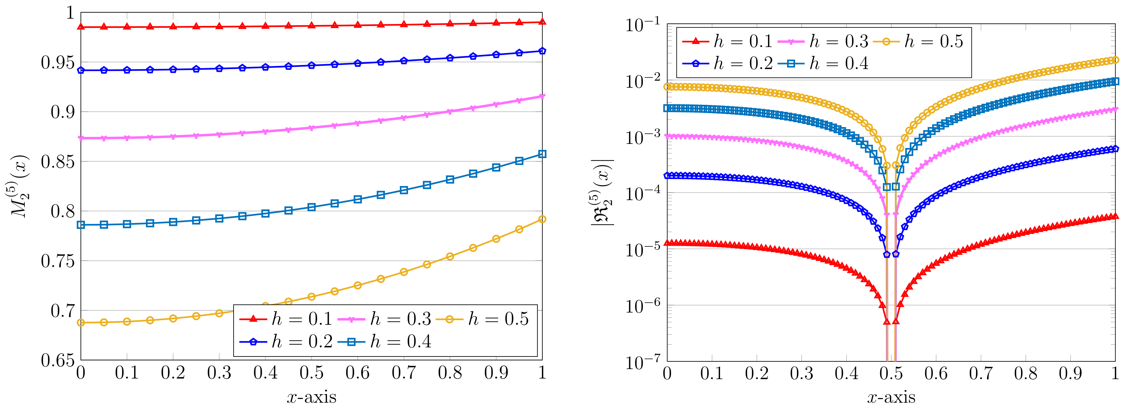
The visualizations of the approximate solutions using different values of are plotted in Figure 1. The absolute error of the associated REFs with these values of H are also exhibited in Figure 1. By looking at this figure demonstrating the closeness of these solutions, we see that the magnitude of REFs are decreased whenever we increase the H. This shows that the proposed method is convergent, and even its tendency to converge is exponential.
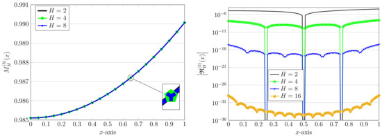
Figure 1.
Approximate solutions (left) and the related absolute values of REFs (right) via the QLM–ChPs approach with , and .
Using the same parameters as above (fixed and ) but with different values of h, we examine the effects of the model parameter h on the computations. The results by using are plotted in Figure 2. The associated REFs are also visualized in the same figure. It is evident that by increasing the parameter h, the corresponding REFs are decreasing in magnitude. This implies that for large values of h, we are required to use a large value of H in the computations to obtain the desired accuracy.
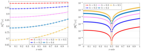
Figure 2.
Approximate solutions (left) and the related absolute values of REFs (right) via the QLM–ChPs approach with , and various .
Let us consider the case of and compare our obtained approximate solution with the outcomes of some existing ones. We obtain the next approximation
which is very close to the output of LWM, reported as [11]
However, one can see a gap between our approximation and that obtained by the ADM [10] given in the form and the solution of CWM [11] obtained as . Again, more alignment will be seen between the approximations obtained by the QLM–ChPs and LWM.
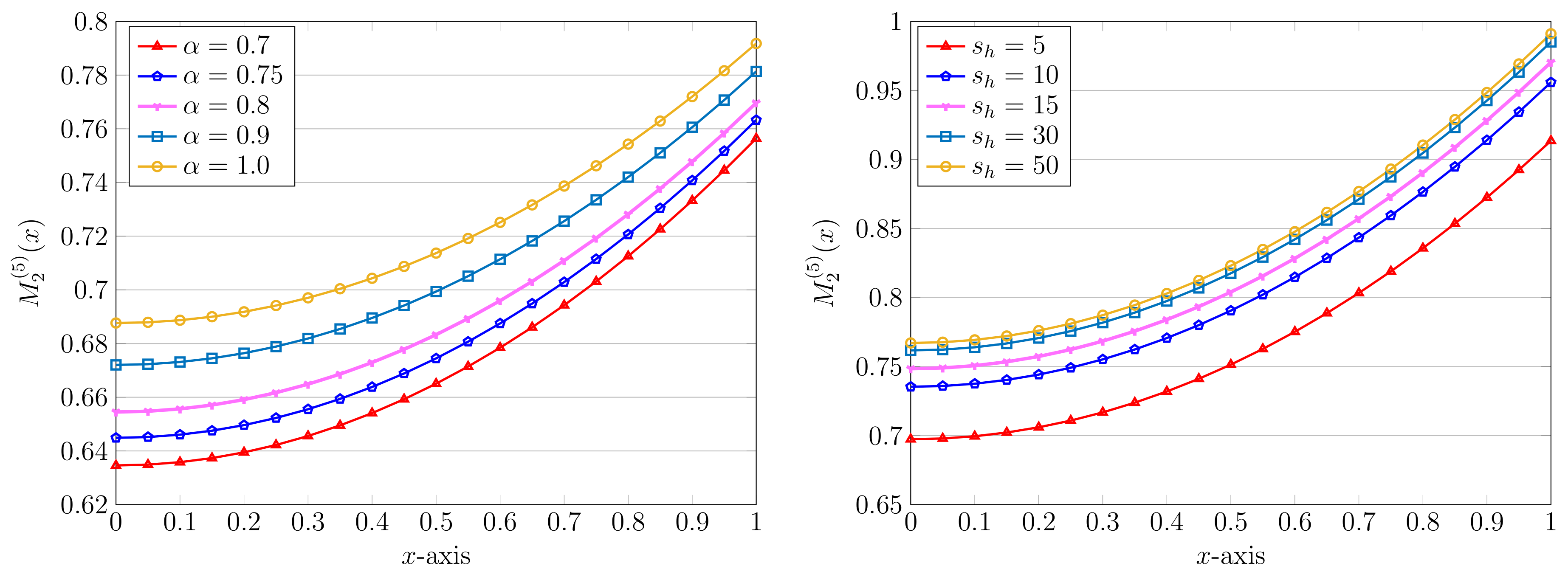
The next simulation results are devoted to the influence of the parameter on the obtained numerical solutions. Towards this end, we first fix and . By taking as before, the approximate solutions for diverse values of and are displayed in Figure 3 (left picture). To be more precise, the approximate solution for is given by
while the corresponding solution obtained by the LWM [11] is .
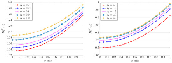
Figure 3.
Approximate solutions using various , , (left) and different , , (right) via the QLM–ChPs approach with .
In the same figure, the right plot, we also show the impact of utilizing various values of the parameter , whereas two other ones are fixed as and . These results by using and for are visualized in this figure. As an example, the result for is as follows:
Here, we can only compute the approximate solution computed by the ADM, which is . We note that the associated REFs for different values of have approximately the same behavior. We thus omitted them to save space. The same was also observed for the achieved REFs related to different in Figure 3.
The next investigation is devoted to the technique of RC. For this purpose, we set . We take all parameters to be united for , and . To start, the approximate solution for is given as
To improve this solution, we need the in the error differential Equation (38). It is given as
We now solve (38) to obtain the error solution , which is obtained as
Consequently, the new approximation is derived by this technique just by adding the previously obtained error term to the preceding approximate solution. It follows that
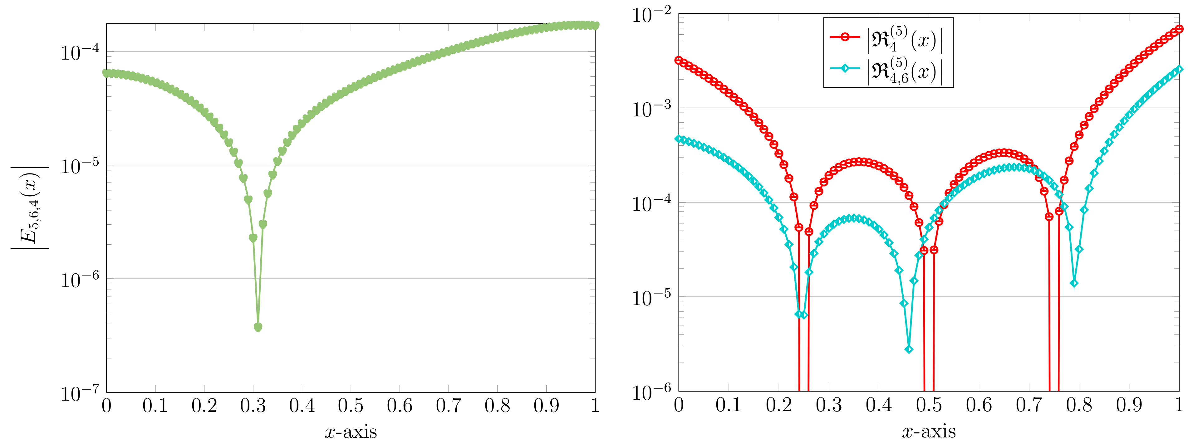
Finally, in the case of and in order to highlight more the difference between the old and new approximations, we present the error solution along with the absolute values of the REFs and . These results are pictured in Figure 4. The precise evaluations of numerical solutions and at some points for are reported in Table 2. We also tabulate the corresponding REFs (in absolute form) in this table for the sake of completeness.
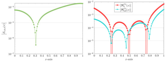
Figure 4.
The error solution (left) and the related absolute values of REFs (right) via the RC technique with and .

Table 2.
Numerical evaluation of approximate solutions and REFs via the RC technique with and at various .
4.2. Case Study II: Spherical Particle ()
Similar to the case of , we start numerical evaluation by fixing the parameters , and using various h as [11]
The approximate solutions by utilizing and these values of h are listed as follows, respectively:
The associated approximations obtained by the ADM [10] and the LWM [11] are also given for comparison purposes as follows:
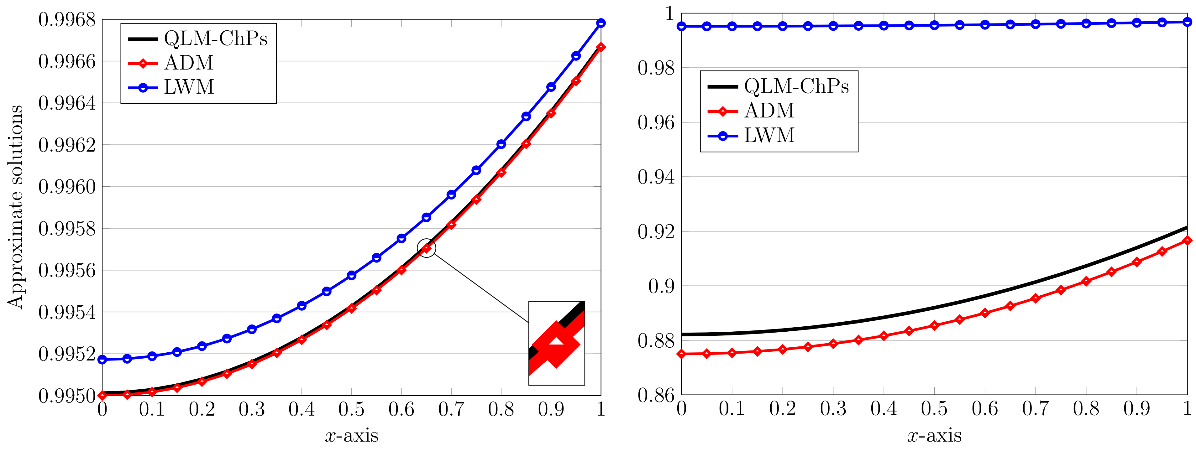
It seems that the agreement between our solutions and two other methods depends heavily on the parameter h. For more insight, let us plot all three numerical solutions using and . Figure 5 shows these approximations together. Clearly, for a small , the outputs of QLM–ChPs and ADM are very close together, while for a larger value , this closeness will be increased. On the other hand, the performance of LWM is poor and our method outperforms the LWM. To confirm the performance of the QLM–ChPs method, we fix and vary . The outcomes presented in Figure 6 show the exponential convergence of our method, which is also simpler in implementation compared to existing ADM and LWM procedures.
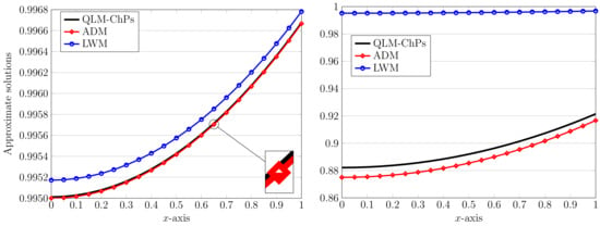
Figure 5.
A comparison of three-term approximate solutions using the ADM/LWM/QLM–ChPs approaches with (left) and (right). In the QLM–ChPs approach, we used and in the spherical case .
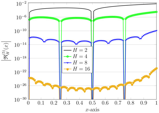
Figure 6.
The absolute values of REFs via the QLM–ChPs approach with , and in the spherical case .
The computed numerical solutions using different and are further presented in Table 3. In this case, we take number of bases. The other parameters are taken as one. Furthermore, the impact of using diverse values of the parameter as well as on the calculated approximation is examined in Figure 7. When these two parameters vary, we take two other ones to be one in the simulations.

Table 3.
The numerical solutions via the QLM–ChPs approach with and various in the spherical case .
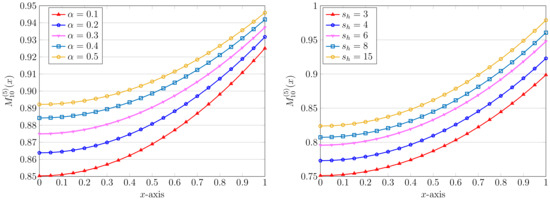
Figure 7.
Approximate solutions using various , , , (left) and different , , (right) via the QLM–ChPs approach with in the spherical case .
Finally, we show the exponential convergence of the proposed QLM–ChPs approach for both case studies I and II related to and respectively. The outcomes of and the corresponding numerical order of convergence (see (41)) for two different values of and are presented in Table 4. For these results, we used , and .

Table 4.
The maximum absolute value of REFs and the associated achieved via the QLM–ChPs procedure using and various H.
5. Conclusions
A class of strongly nonlinear BVPs with singularity arising in the modeling of a reaction and diffusion process with Michaelis–Menten kinetics has been investigated in this research study. To obtain a polynomial solution for the model equation, the technique of spectral matrix collocation together with the quasilinearization strategy was proposed efficiently and accurately. In this respect, a new class of polynomials related to the well-known Bessel functions of Krall–Frink was used in the collocation procedure. In the norm, we derived an upper bound for the error related to these polynomials theoretically. Several numerical test examples with all values of parameters were solved to acquire the (steady-state) substrate concentrations in a solid with planar and spherical shape, approximately. Comparisons with the outputs of two existing methods, namely, the Adomian decomposition approach and wavelet-based procedures, have been made to show the validity of the combined QLM–ChPs algorithm. The techniques of residual error functions and the error correction were employed to check the accuracy of the obtained solutions in the absence of the exact solutions. The latter technique further helped us to improve the quality of obtained approximations. The presented outcomes shown by tables and figures confirm that the QLM–ChPs technique is not only highly accurate and efficient but also capable of solving various similar model problems with strong nonlinearity and singularity.
Author Contributions
Conceptualization, M.I. and H.M.S.; methodology, M.I. and H.M.S.; software, M.I.; validation, M.I. and H.M.S.; formal analysis, M.I. and H.M.S.; funding acquisition, H.M.S.; investigation, M.I. and H.M.S.; writing—original draft preparation, M.I.; writing—review and editing, M.I. and H.M.S. All authors have read and agreed to the published version of the manuscript.
Funding
This research received no external funding.
Institutional Review Board Statement
Not applicable.
Informed Consent Statement
Not applicable.
Data Availability Statement
Not applicable.
Conflicts of Interest
The authors declare no conflict of interest.
References
- Scheller, F.; Schubeert, F. Biosensor; Elsevier: Amsterdam, The Netherlands, 1988; Volume 7. [Google Scholar]
- Wollenberger, U.; Lisdat, F.; Scheller, F.W. Enzymatic Substrate Recycling Electrodes. Frontiers in Biosensorics. B and II, Practical Applications; Birkhauser Verlag: Basel, Switzerland, 1997; pp. 45–70. [Google Scholar]
- Aris, R. Mathematical Modeling: A Chemical Engineer’s Perspective; Elsevier: Amsterdam, The Netherlands, 1999. [Google Scholar]
- Michaelis, L.; Menten, M. Die kinetic der invertinwirkung. Biochem. Z. 1913, 79, 333–369. [Google Scholar]
- Lin, S.H. Oxygen diffusion in a spherical cell with nonlinear oxygen uptake kinetics. J. Theoret. Biol. 1976, 60, 449–457. [Google Scholar] [CrossRef] [PubMed]
- McElwain, D.L.S. A Re-examination of oxygen diffusion in a spherical cell with Michaelis–Menten oxygen uptake kinetics. J. Theoret. Biol. 1978, 7, 255–263. [Google Scholar] [CrossRef] [PubMed]
- Manimozhi, P.; Subbiah, A.; Rajendran, L. Solution of steady-state substrate concentration in the action of biosensor response at mixed enzyme kinetics. Sens. Actuators B Chem. 2010, 14, 290–297. [Google Scholar] [CrossRef]
- Indira, K.; Rajendran, L. Analytical expression of the concentration of substrates and product in phenol-polypheneol oxidase system immobilized in laponite hydrogels Michaelis-Menten formalism in homogeneous medium. Electrochim. Acta 2011, 56, 6411–6419. [Google Scholar] [CrossRef]
- Merchant, T.R. Cubic autocatalysis with Michaelis-Menten kinetics: Semi-analytical solutions for the reaction-diffusion cell. J. Chem. Eng. Sci. 2004, 59, 3433–3440. [Google Scholar] [CrossRef]
- Devi, M.R.; Sevukaperumal, S.; Rajendran, L. Non-linear reaction diffusion equation with Michaelis-Menten kinetics and Adomian decomposition method. Appl. Math. 2015, 5, 21–32. [Google Scholar]
- Mahalakshmi, M.; Hariharan, G.; Brindha, G.R. An efficient wavelet-based optimization algorithm for the solutions of reaction-diffusion equations in biomedicine. Comput. Methods Progams Biomed. 2021, 186, 105218. [Google Scholar] [CrossRef]
- Tosaka, N.; Miyale, S. Analysis of a nonlinear diffusion problem with Michaelis Menten kinetics by an integral equation method. Bull. Math. Biol. 1982, 44, 841–849. [Google Scholar] [CrossRef]
- Simpson, M.J.; Ellery, A.J. An analytical solution for diffusion and nonlinear uptake of oxygen in a spherical cell. Appl. Math. Model. 2012, 36, 3329–3334. [Google Scholar] [CrossRef]
- Selvi, M.S.M.; Seethalakshmi, R.; Rajendran, L. An analytical solution for diffusion and nonlinear uptake of oxygen in a planar, cylindrical and spherical cell using wavelet method. J. Crit. Rev. 2020, 7, 9729–9744. [Google Scholar]
- Singh, R.; Wazwaz, A.M. Optimal homotopy analysis method for oxygen diffusion in a spherical cell with nonlinear oxygen uptake kinetics. MATCH Commun. Math. Comput. Chem. 2018, 80, 369–382. [Google Scholar]
- Hadhoud, A.R.; Ali, K.K.; Shaalan, M.A. A septic B-spline collocation method for solving nonlinear singular boundary value problems arising in physiological models. Sci. Iran. 2020, 27, 1674–1874. [Google Scholar]
- Roul, P. A new mixed MADM-collocation approach for solving a class of Lane–Emden singular boundary value problems. J. Math. Chem. 2019, 57, 945–969. [Google Scholar] [CrossRef]
- Tripathi, V.M.; Srivastava, H.M.; Singh, H.; Swarup, C.; Aggarwal, S. Mathematical analysis of non-isothermal reaction-diffusion models arising in spherical catalyst and spherical biocatalyst. Appl. Sci. 2021, 11, 10423. [Google Scholar] [CrossRef]
- Jamal, B.; Khuri, S.A. Non-isothermal reaction-diffusion model equations in a spherical biocatalyst: Green’s function and fixed point iteration approach. Int. J. Appl. Comput. Math. 2019, 5, 120. [Google Scholar] [CrossRef]
- Abuasbeh, K.; Qureshi, S.; Soomro, A.; Awadalla, M. An optimal family of block techniques to solve models of infectious diseases: Fixed and adaptive stepsize strategies. Mathematics 2023, 11, 1135. [Google Scholar] [CrossRef]
- Qureshi, S.; Ramos, H. L-stable explicit nonlinear method with constant and variable step-size formulation for solving initial value problems. Int. J. Nonlinear Sci. Numer. Simul. 2018, 19, 741–751. [Google Scholar] [CrossRef]
- Aydinlik, S. An efficient method for oxygen diffusion in a spherical cell with nonlinear oxygen uptake kinetics. Int. J. Biomath. 2022, 15, 2250019. [Google Scholar] [CrossRef]
- Izadi, M.; Yüzbası, S.; Cattani, C. Approximating solutions to fractional-order Bagley-Torvik equation via generalized Bessel polynomial on large domains. Ricerche Mat. 2023, 72, 235–261. [Google Scholar] [CrossRef]
- Yüzbası, S.; Yildirim, G. A Laguerre approach for solving of the systems of linear differential equations and residual improvement. Comput. Methods Differ. Equ. 2021, 9, 553–576. [Google Scholar]
- Abd-Elkawy, M.A.; Alqahtani, R.T. Shifted Jacobi spectral collocation method for solving two-sided fractional water wave models. Europ. Phys J. Plus 2017, 132, 50. [Google Scholar] [CrossRef]
- Youssri, Y.H.; Hafez, R.M. Exponential Jacobi spectral method for hyperbolic partial differential equations. Math. Sci. 2019, 13, 347–354. [Google Scholar] [CrossRef]
- Abd-Elhameed, W.M.; Al-Harbi, M.S.; Amin, A.K.; Ahmed, H.M. Spectral treatment of high-order Emden-Fowler equations based on modified Chebyshev polynomials. Axioms 2023, 12, 99. [Google Scholar] [CrossRef]
- Srivastava, H.M.; Izadi, M. The Rothe-Newton approach to simulate the variable coefficient convection-diffusion equations. J. Mahani Math. Res. 2022, 11, 141–157. [Google Scholar]
- Yadav, P.; Jahan, S.; Nisar, K.S. Solving fractional Bagley-Torvik equation by fractional order Fibonacci wavelet arising in fluid mechanics. Ain Shams Eng. J. 2023, 14, 102299. [Google Scholar] [CrossRef]
- Izadi, M.; Zeidan, D. A convergent hybrid numerical scheme for a class of nonlinear diffusion equations. Comp. Appl. Math. 2022, 41, 318. [Google Scholar] [CrossRef]
- Srivastava, H.M.; Adel, W.; Izadi, M.; El-Sayed, A.A. Solving some physics problems involving fractional-order differential equations with the Morgan-Voyce polynomials. Fractal Fract. 2023, 7, 331. [Google Scholar] [CrossRef]
- Krall, H.L.; Frink, O. A new class of orthogonal polynomials: The Bessel polynomials. Trans. Amer. Math. Soc. 1949, 65, 100–115. [Google Scholar] [CrossRef]
- Chatterjea, S.K. New class of polynomials. Ann. Mat. Pura Appl. 1964, 65, 35–48. [Google Scholar] [CrossRef]
- Izadi, M.; Srivastava, H.M.; Adel, W. An effective approximation algorithm for second-order singular functional differential equations. Axioms 2022, 11, 133. [Google Scholar] [CrossRef]
- Izadi, M.; Roul, P. Spectral semi-discretization algorithm for a class of nonlinear parabolic PDEs with applications. Appl. Math. Comput. 2022, 429, 127226. [Google Scholar] [CrossRef]
- Izadi, M.; Srivastava, H.M. Applications of modified Bessel polynomials to solve a nonlinear chaotic fractional-order system in the financial market: Domain-splitting collocation techniques. Computation 2023, 11, 130. [Google Scholar] [CrossRef]
- Srivastava, H.M. An introductory overview of Bessel polynomials, the generalized Bessel polynomials and the q-Bessel polynomials. Symmetry 2023, 15, 822. [Google Scholar] [CrossRef]
- Izadi, M. A combined approximation method for nonlinear foam drainage equation. Sci. Iran. 2022, 29, 70–78. [Google Scholar]
- Aznam, S.M.; Ghani, N.A.; Chowdhury, M.S. A numerical solution for nonlinear heat transfer of fin problems using the Haar wavelet quasilinearization method. Results Phys. 2019, 14, 102393. [Google Scholar] [CrossRef]
- Izadi, M.; Srivastava, H.M. Robust QLM-SCFTK matrix approach applied to a biological population model of fractional order considering the carrying capacity. Discrete Contin. Dyn. Syst. Ser. S 2023, 2023, 1–23. [Google Scholar] [CrossRef]
Disclaimer/Publisher’s Note: The statements, opinions and data contained in all publications are solely those of the individual author(s) and contributor(s) and not of MDPI and/or the editor(s). MDPI and/or the editor(s) disclaim responsibility for any injury to people or property resulting from any ideas, methods, instructions or products referred to in the content. |
© 2023 by the authors. Licensee MDPI, Basel, Switzerland. This article is an open access article distributed under the terms and conditions of the Creative Commons Attribution (CC BY) license (https://creativecommons.org/licenses/by/4.0/).


