Article

Feasibility Analysis of Online Uncertainty Metrics for PMU-Based State Estimation

by
Guglielmo Frigo
1,* and
Federico Grasso-Toro
2
1
Swiss Federal Institute of Metrology METAS, Lindenweg 50, 3007 Bern-Wabern, Switzerland
2
Open-Science Team, University of Bern, Hochschulstrasse 6, 3012 Bern, Switzerland
*
Author to whom correspondence should be addressed.
Appl. Sci. 2023, 13(21), 11670; https://doi.org/10.3390/app132111670
Submission received: 8 September 2023 / Revised: 16 October 2023 / Accepted: 23 October 2023 / Published: 25 October 2023

Abstract

:
The ever-increasing penetration of renewable energy sources and distributed generation needs developing and deploying more sophisticated and precise control techniques. The paradigm shift from high-rotational inertia towards inverter-connected facilities has made modern power systems subject to strongly non-stationary operating conditions. In this context, phasor measurement units (PMUs) represent a promising solution due to their accuracy and time synchronization. The current paper further develops the concepts recently published proposing performance assessment of PMUs relying on metrics specifically defined to quantify the estimation accuracy, reporting latency, and response time. Our focus is on determining the confidence interval associated with these metrics and thus derive a robust approach for their application in measurement-based network controlling efforts. The configuration of the used simulation model is detailed, and the state estimation results as a function of the selected measurement weighing criteria are presented, concluding as a possible application of the reliability metrics in Weighted Least Squares and Discrete Kalman Filter state estimators, highlighting the performance enhancement as well as the theoretical limits of the proposed approach.

1. Introduction

In recent years, the ever-increasing penetration of renewable energy sources and distributed generation is pushing for the development and deployment of more sophisticated and precise control techniques [1,2,3]. Due to the loss of rotational inertia in favor of inverter-connected facilities, modern power systems are subject to strongly non-stationary operating conditions, characterized by fast dynamics and wide-band spectrum [4].
In this context, the measurement infrastructure is expected to become the backbone of many monitoring and control applications [5], as state estimation [6], fault location [7], loss-of-mains detection [8], and under-frequency load shedding [9]. To this end, Phasor Measurement Units (PMUs) represent a promising solution due to their measurement accuracy and time synchronization [10,11]. In compliance with the recent IEC Std 60255-118-1 (briefly, IEC Std) [12], PMUs measure the phasor, frequency, and rate of change of frequency (ROCOF) of the fundamental component with reporting rates in the order of tens of frames per second.
The National Metrology Institutes (NMIs) are responsible for the rigorous characterization and precise calibration of PMUs [13,14]. In this sense, the IEC Std introduces two performance classes, P and M, intended for protection and measurement applications. The first one has higher responsiveness, whereas the second one is required higher accuracy. The performance assessment relies on metrics specifically defined to quantify the estimation accuracy, reporting latency, and response time of the PMU. In particular, the estimation accuracy is defined in terms of Total Vector Error (TVE), Frequency Error (FE), and ROCOF Error (RFE).
However, the entire IEC Std theoretical framework relies on a static and stationary signal model that cannot fully represent the dynamics of modern power systems. Hence, recent literature has explored extending or overcoming the phasor signal model in favor of more sophisticated approaches capable of properly capturing wide-bandwidth phenomena [15,16]. Nevertheless, the transition from PMUs (and similar phasor-based devices) to a new generation of instruments is neither envisioned nor expected to be completed for a long time. Therefore, the role of NMIs is to evaluate the measurement uncertainty caused by the modeling discrepancy between the signal model and the signal under test and determine plausible confidence intervals for PMU-based control applications. A typical example in this sense is represented by the regulations regarding ROCOF withstand capability for connecting new power-generating modules or demand units [17].
An alternative approach is to identify new performance metrics that do not suffer from the same definitional uncertainty [18], e.g., by considering the signal in the time domain where the only limitation is represented by the amplitude and time resolution of the acquired time series. In this context, two promising metrics have been introduced, namely the Goodness-of-Fit (GoF) [19] and the Normalized Root Mean Squared Error (nRMSE) [20].
Similarly, both these metrics quantify how much of the original signal energy has been neglected by the corresponding phasor representation [21]. The larger the residual energy, the lower the reliability of the PMU estimates.
A recent publication has discussed the variation range and the estimation uncertainty inherent in these metrics. It has proposed a possible standard amendment that would allow transmitting its value with the PMU estimates [22]. Indeed, the IEC Std format for the measurement data packet already contains a few bit-mapped flags defining the instrument’s internal state and the measurement quality info. Without affecting the overall packet size, it would be possible to transmit the reliability metric value at the cost of an extra 4 bytes and thus make it available to the applications processing the PMU estimates.
The knowledge of this reliability metric opens up new possibilities at different network levels. It can be seen as a flag of possible instrument failure at the sensor level. At a higher and aggregated level, it can detect faults or anomalies. In this regard, this information has been proven to be capable of improving the accuracy in fault location applications [23].

Paper Contributions

In this context, the present paper investigates the feasibility of using the reliability metric in PMU-based state estimation applications. By extending the analysis presented in [24], we assess the confidence interval of the selected metric as a function of their mathematical definition and the considered operating conditions. This way, we identify which uncertainty contributions are suitably quantified and which are neglected or misrepresented.
To the state-of-the-art, the reliability metrics have been employed for a posteriori analysis of unexpected estimate distribution or contingencies. In this paper, we propose an online application where each metric is computed locally and then employed globally to minimize the impact of definitional uncertainty effects.
In more detail, we consider two well-known state estimation approaches, namely Weighted Least Squares (WLS) and Discrete Kalman Filter (DKF) [25,26]. The choice of these two approaches is not only based on their popularity and wide employment in many state estimation approaches. Indeed, WLS and DKF allow us to account for the measurement uncertainty directly in the problem statement. Instead of considering predefined and constant criteria (e.g., the instrument transformer class), the uncertainty associated with each measurement is assessed online and directly included in the state estimation routine.
We do not consider purely standard conditions for this analysis, but we reproduce a more realistic operating scenario. In the MATLAB R2022b Simulink environment, we simulate the well-known IEEE 14-bus system [27], and populate it with PMU models compliant with the IEC Std requirements [28]. By substituting the original load with non-linear time-varying models, we can reproduce dynamic conditions compatible with high shares of renewable energy sources. Throughout extensive numerical simulations, we highlight the proposed approach’s performance enhancement and theoretical limits. The statistical distribution of the state estimation errors confirms how the most limiting factor is represented by the improper assumption of constant PMU reliability, independently from the current operating condition. We also validated this consideration by applying a different model of the instrument transformer contributions.
The paper is organized as follows. Section 2 presents the main uncertainty contributions inherent in any PMU-based measurement chain. In Section 3, we introduce the online performance metric to assess modeling inconsistencies between measurand and reference signal model and characterize its statistical distribution in operating conditions inspired by real-world data sets. Section 4 describes the configuration of the simulation model and discusses the most suitable setting of its main parameter values. In Section 5, we present the state estimation results as a function of the selected measurement weighing criteria. Finally, Section 6 provides some closing remarks.

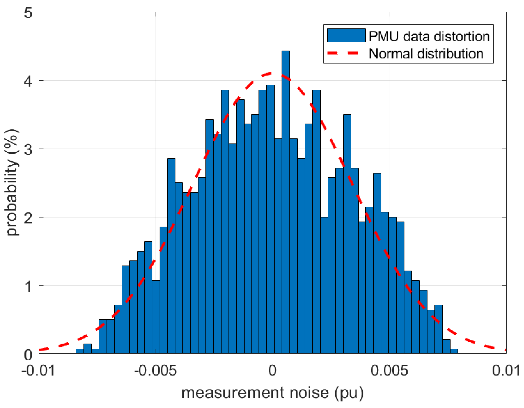
2. Uncertainty Contributions in the PMU Measurement Chain

A PMU-based measurement system is comprised of several components, each characterized by specific properties and functions. In this sense, we can identify three main components. The Instrument Transformer (IT) stage converts the voltage and current signals of interest into a range compatible with the PMU analog front-end. The PMU acquires the IT secondary signals and processes them to produce time-stamped estimates of phasor, frequency, and ROCOF. A synchronization source guarantees the time-stamp alignment to the Universal Coordinated Time (UTC).
Each component contributes to the overall uncertainty of the measurement chain and is regulated by specific standards and performance requirements. From a metrological point of view, it is important to classify the different uncertainty contributions and to define the most suitable tests and methods to rigorously assess them.
In this context, Figure 1 proposes a possible classification of the uncertainties inherent in a PMU-based measurement system. It is worth noticing that such a classification is neither univocal nor standardized. Still, it takes inspiration from the similar classification employed for Power Quality (PQ) meters in the IEC Std 62586-2 [29]. The so-called intrinsic uncertainty accounts for the PMU performance in nominal conditions, which can usually be deduced from the manufacturer’s specifications. The measurement uncertainty considers the contribution of power system variations and is assessed in the IEC Std tests. Finally, the overall uncertainty also considers the contribution of all non-PMU components, such as the synchronization source or the IT class.
This last component is typically way larger than the others and dominates the overall uncertainty budget. For this reason, in the absence of more specific information, the IT class is traditionally considered a reliability metric of the PMU-based measurement result and used as a weight in WLS or DKF state estimators. Such an approach yields pros and cons. On the one hand, it accounts for the most significant source of uncertainty. On the other hand, though, it relies on a priori and sporadically updated information like the IT class. Consequently, the weight associated with a single measurement result is constant and totally independent of the current operating conditions.

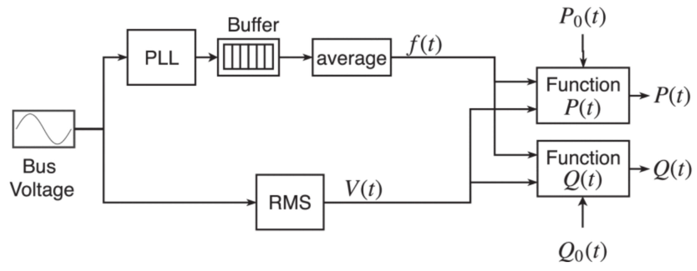
3. Online Performance Assessment

In the considered low-inertia scenario, a generic power signal can be represented by a non-linear dynamic model:
x ( t ) = A · 1 + ε A ( t ) · cos 2 π f t + φ + ε φ ( t ) + η ( t ) + z ( t )
where A, f, and φ are the fundamental component’s amplitude, frequency, and initial phase, respectively. The time-varying terms ε A and ε φ account for amplitude and phase dynamics in terms of polynomial, exponential, or modulation trends. The additive terms η and z represent the spurious contribution of narrow- and wide-band disturbances, respectively. More in detail, the first refers to the combination of harmonic and inter-harmonic terms, whereas the second accounts for continuous-spectrum components as white or colored noise, decaying DC, or transients.
In any PMU-based measurement system, the first step of the measurement chain consists of the acquisition process:
x [ n ] x ( t = n T s ) , T s = F s 1 , n = 1 , N s
where F s is the sampling rate, and N s is the sample length. It is worth noticing that such equality represents just an approximation, as it does not account for the quantization errors, the distortion introduced by the instrument transformer and the analog front-end, or the phase noise caused by the non-perfectly uniform sampling rate [30]. On the other hand, the dynamics considered in this paper are likely to affect the considered performance metric more significantly, as further proven in the following Section, making these uncertainty contributions negligible for the considered application.
Given the acquired sample series, the PMU is required to estimate the synchrophasor p ^ , frequency f ^ , and ROCOF R ^ f associated with the fundamental component:
p ^ [ m ] = A ^ [ m ] · exp j · 2 π ( f ^ [ m ] f 0 ) m T r + φ ^ [ m ]
where the superscript indicates the estimated parameters, while T r and m are the reporting period and the reporting index, respectively. The subtraction by the system-rated frequency f 0 allows for expressing the phase contribution due to off-nominal signal frequencies.
It is worth observing that the phasor signal model assumes that the signal energy is stationary within the considered observation interval and that the signal energy is mostly concentrated in a narrow bandwidth around the fundamental frequency. When these assumptions are not met (e.g., during an instantaneous step change of amplitude or phase), the PMU estimates suffer from definitional uncertainty due to the model inconsistency between the spectral properties of the signal under test and its phasor representation [31].
Consequently, the recent literature has discussed the metrological significance of standard performance metrics in real-world operating conditions and approaches for assessing PMU reliability during transient conditions. In particular, two novel metrics have been introduced: the GoF and the nRMSE. Both are defined in the time domain and do not rely on the phasor signal model, and they do not introduce any constraint regarding the spectral bandwidth of the observed phenomenon.
Based on the PMU estimates, it is possible to recover the time-domain trend of the fundamental component as:
x ^ [ n ] = A ^ · cos 2 π f ^ n T s + φ ^ + π R ^ f ( n T s ) 2
and define its discrepancy with respect to the corresponding acquired sample series in terms of two similar metrics:
n R M S E = ( x ^ [ n ] x [ n ] ) 2 N s
G o F = A ^ ( x ^ [ n ] x [ n ] ) 2 N s d
where d is the model degrees of freedom (typically equal to 3, as R ^ f is derived as a finite difference of consecutive frequency estimates). If we consider the PMU estimation as a non-linear fit process, both the metrics quantify the residuals’ energy, which can be interpreted as an assessment of the signal energy (and thus signal information content) that has been neglected or misrepresented due to the inconsistency between phasor model and acquired sample series.
For the sake of brevity, the analysis considers the nRMSE metric only as its definition is slightly more general, not requiring the knowledge a priori of the model degrees of freedom. Nevertheless, similar considerations also hold for the GoF metric. In the following, we consider PMU-based measurements of voltage and current phasors as they are easily referable to a well-defined signal model, but similar approaches might be applied also to other types of measurements in a SCADA system.

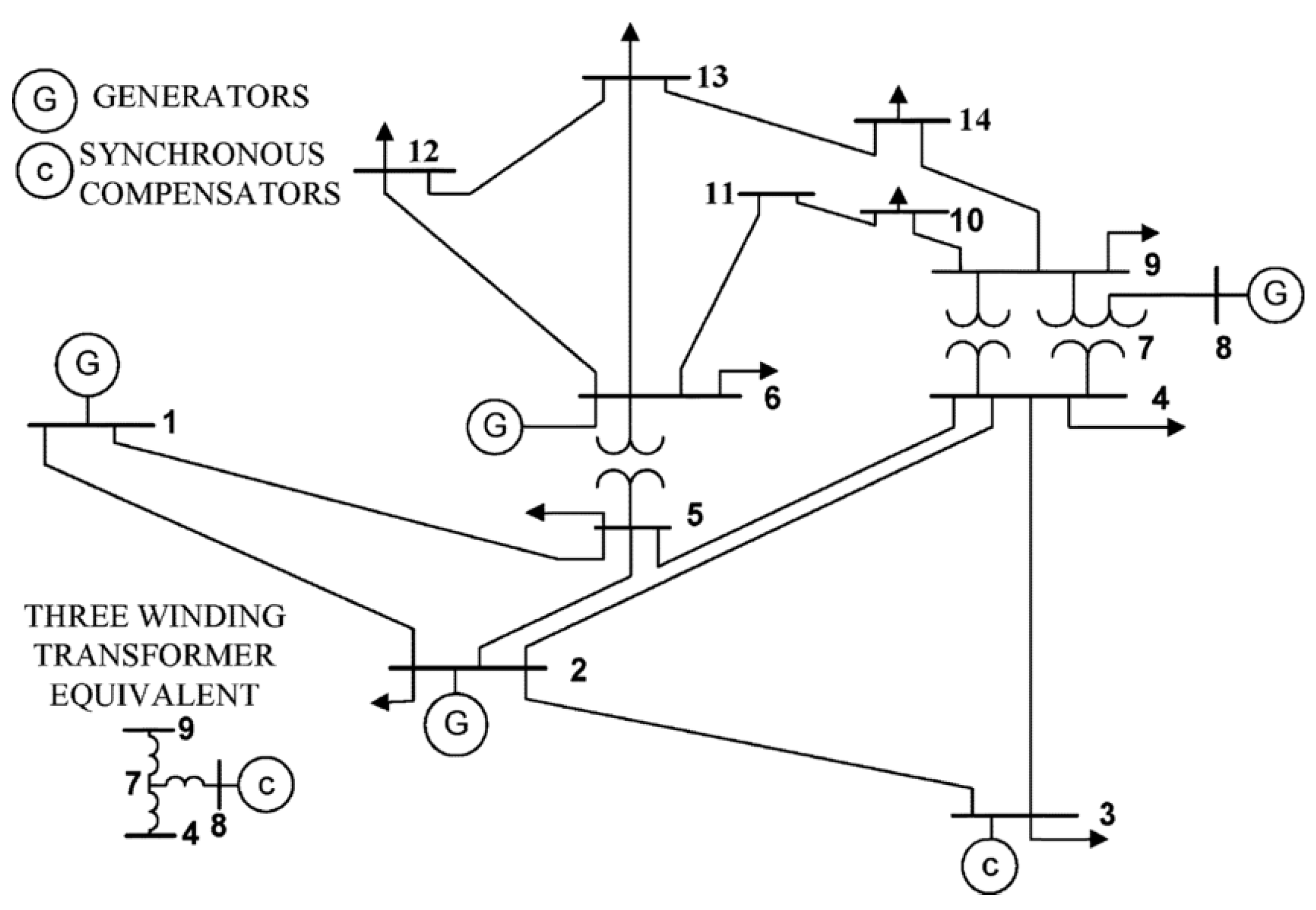
4. State Estimation Scenario

In the MATLAB Simulink programming environment, we reproduce the IEEE 14-bus test case. For completeness, the one-line diagram of the network is reported in Figure 2. It is worth noticing that the IEEE 14-bus test case represents a portion of the American electric power system (in the Midwestern US) as of February 1962. It consists of fourteen buses and five generators (without loss of generality, the nominal system rate has been set equal to 50 Hz. Nevertheless, similar results are expected in a 60-Hz scenario), and 11 loads [27].
In each bus, we deployed a PMU model that measures both voltage and current phasors. In more detail, the PMU implements a dynamic phasor estimator, namely the Compressive Sensing Taylor-Fourier Multifrequency (CS-TFM) model, that guarantees a remarkable performance in the presence of time-varying and highly distorted conditions. For this analysis, the PMU is set in P-class configuration, with a sampling rate of 5 kHz, an observation interval of 60 ms, and a reporting rate of 50 frames per second (fps).
The CS-TFM is a dynamic estimator, i.e., it recovers not only the fundamental synchrophasor but also its first- and second-order derivatives as computed around the reporting time instant. The time-domain trend of the fundamental component can be thus computed in two ways:
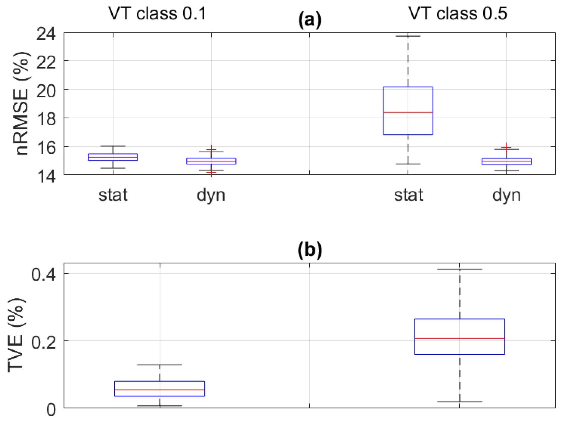
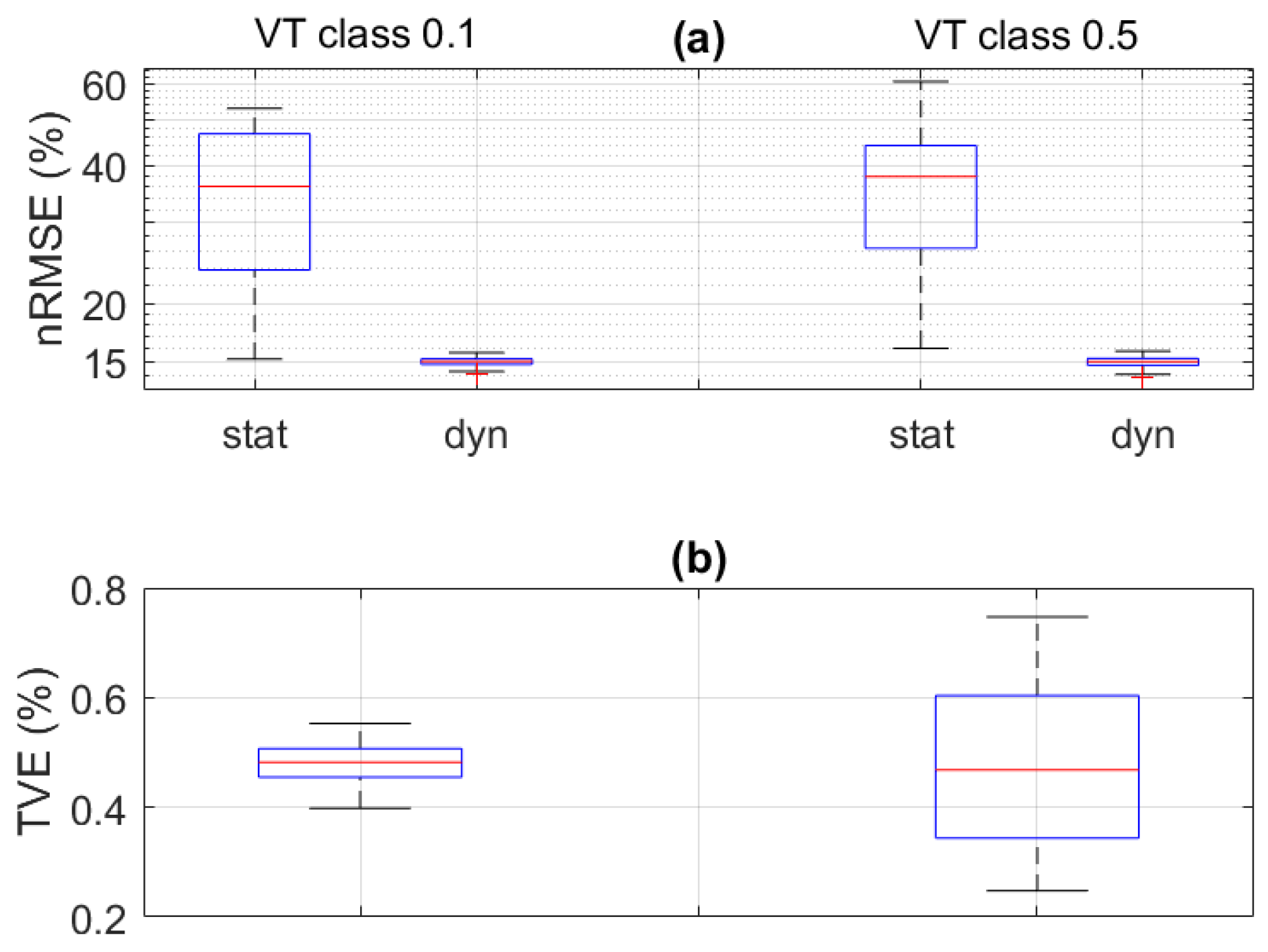
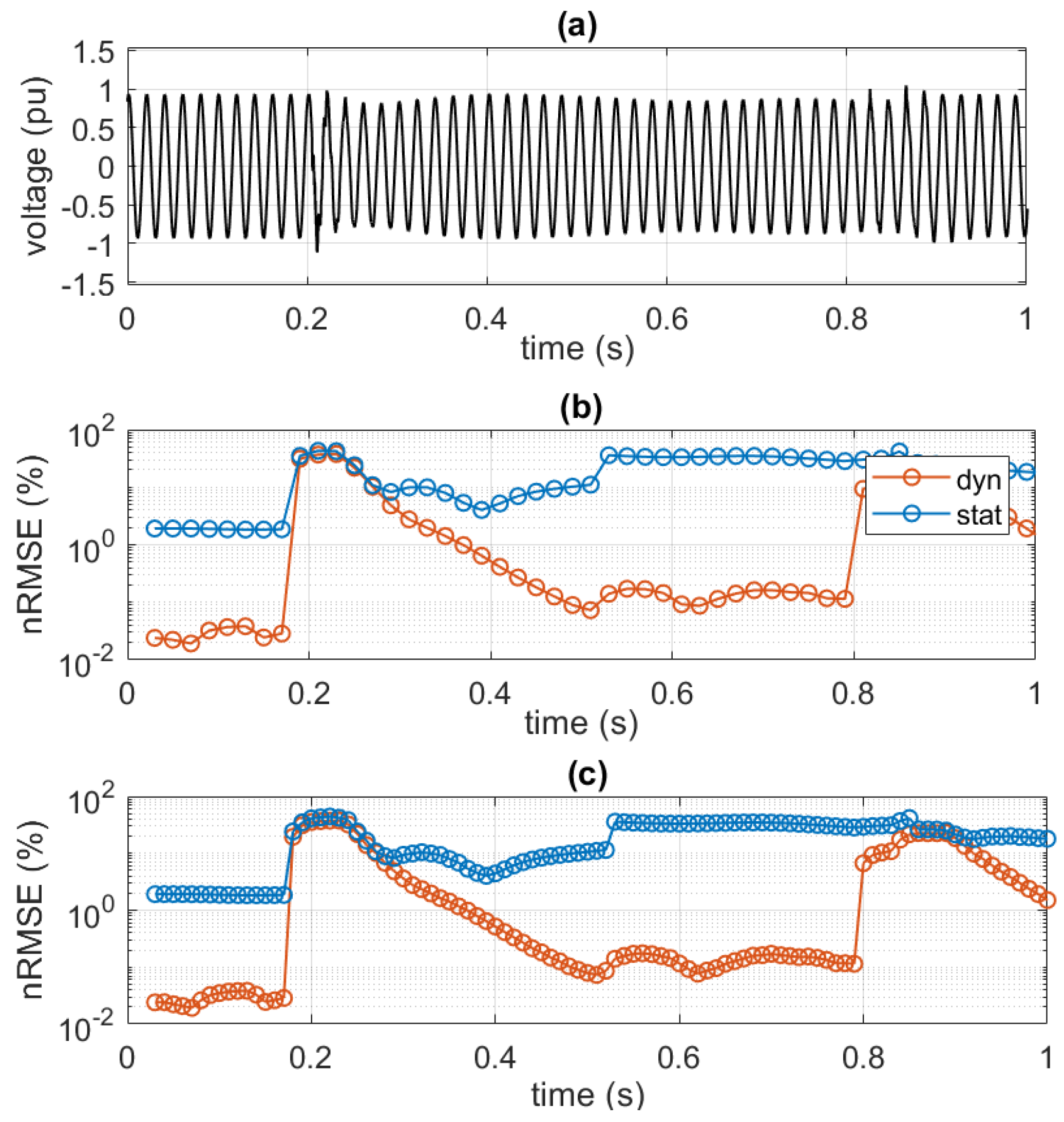
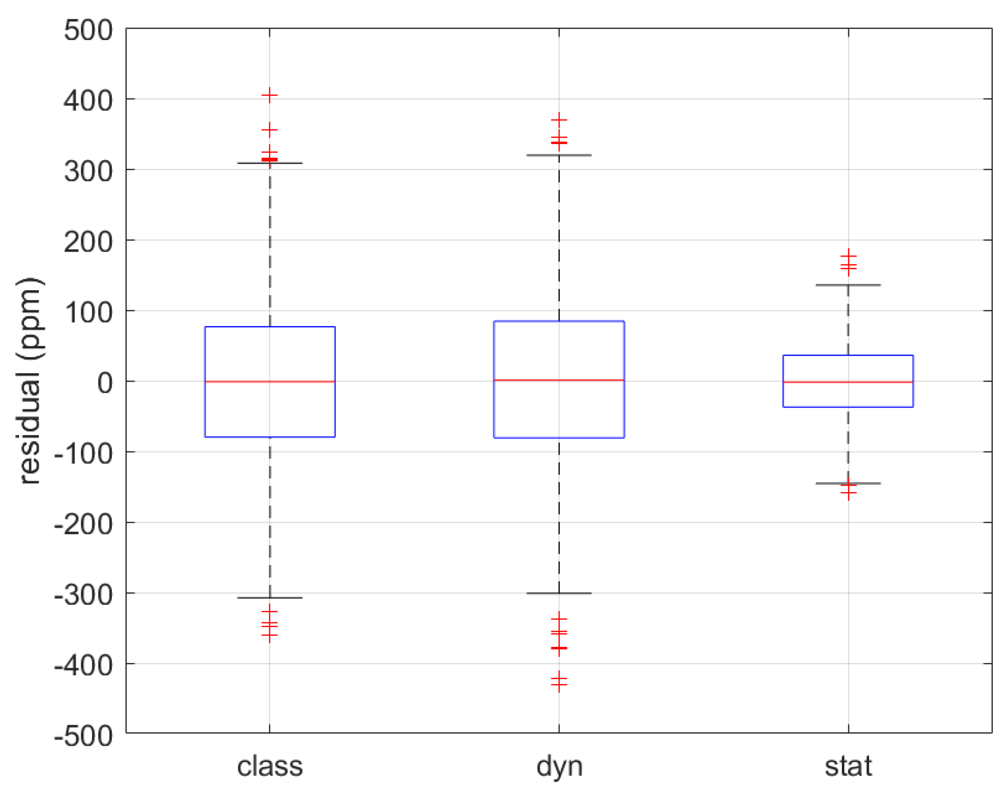
  • static: considering only the zero-order parameters, i.e., amplitude, frequency, phase, and ROCOF, as in (4);
  • dynamic: considering all the derivative terms, i.e., accounting also for the parameter variations within the considered window.
As further discussed in the following Section, the different formulations result in different nRMSEs and consequent considerations. In the static case, we measure the estimation reliability of the IEC Std parameters, whereas in the dynamic case, we evaluate how much the dynamic model is capable of tracking their time variations. A window of 60 ms is required to guarantee optimal performance. In a Real-Time implementation, the estimation time is circa 20 μ s.
The measurement uncertainty inherent in the PMU acquisition process is modeled through two independent contributions: the distortion due to wide- and narrow-band disturbances and the systematic error introduced by the instrument transformer. The wide-band distortion is modeled as additive white Gaussian noise, such that the Signal-to-Noise ratio is equal to 45 and 35 dB for voltage and current waveforms, respectively.
Such values are taken from an experimental data set of real-world waveforms directly acquired on the EPFL campus. In a similar way, the narrow-band distortion is modeled as a linear combination of the first 40 harmonic terms, whose amplitude is randomly selected in order to reproduce an overall Total Harmonic Distortion (THD) ratio of 0.75 and 14.50% for voltage and current waveforms, respectively, as inferred from the spectral analysis performed on the same data set [32].
As regards the instrument transformers, in this stage of the research, we consider only the systematic error contributions, as we assume that the non-linear effects are covered by noise and harmonics [33]. For this analysis, we consider two performance classes for both current and voltage transformers. Table 1 reports the maximum systematic error in terms of ratio Δ ε and phase error Δ φ for the different transformer classes and the interested nodes. From an implementation point of view, systematic errors are applied to each PMU estimate, assuming a uniform distribution with a variance equal to one-third of the squared maximum error [34].
In order to reproduce dynamic operating conditions, the loads have been simulated according to the EPRI LOADSYN model [35]. In particular, the three-phase active and reactive power are modeled as the functions of time P ( t ) and Q ( t ) :
P ( t ) = P 0 ( t ) · V ( t ) V 0 K p v · 1 + K p f · ( f ( t ) f 0 ) Q ( t ) = Q 0 ( t ) · V ( t ) V 0 K q v · 1 + K q f · ( f ( t ) f 0 )
where the voltage and frequency sensitivity parameters K p v = 1.7 , K p f = 1.0 , K q v = 2.6 , and K q f = 1.7 are based on typical values as inferred from the EPRI LOADSYN program. The instantaneous frequency f ( t ) and voltage V ( t ) , as well as the rated profiles of active P 0 ( t ) and reactive power Q ( t ) are updated with the same reporting rate of the PMUs, i.e., every 20 ms. In this way, by varying the rated profiles, it is possible to reproduce different dynamic scenarios. A constant profile results in a quasi-stationary condition, whereas profiles taken from real-world acquisitions can be employed to reproduce more challenging and dynamic conditions.
In order to avoid recursive and diverging effects, the frequency and voltage measurements do not come from the PMUs. As shown in Figure 3, the frequency is measured by a Phase Locked Loop (PLL) followed by a moving average filter to reduce spurious oscillations, whereas the voltage is given by a Root Mean Square (RMS) operator. Both the moving average filter and the RMS operator consider observation intervals of 240 ms, that are suitably partially overlapped in order to reproduce a reporting rate of 50 fps.

5. Simulation Results

5.1. Sensitivity Analysis

In the first test, we perform a sensitivity analysis of the nRMSE metric as a function of the test conditions and of the reconstruction model. For this analysis, we consider two test signals. The first one is in quasi-steady-state (SS) conditions. The amplitude and initial phase are stationary and equal to their nominal value (for simplicity, 1 pu and 0 rad, respectively), whereas the frequency is initiated at 50 Hz, but its time dependence is modeled as a random walk process with a variance of 1 μ Hz. This reproduces the typical variability due to the continuous adjustment of the power generation and demand profiles.
The second signal adds a further level of complexity by introducing a phase modulation (PM) with a modulation depth and frequency equal to π / 10 rad and 2 Hz, respectively. As a consequence, the erratic trend of the instantaneous frequency is super-posed to a sinusoidal oscillation of ± 0.628 Hz every 0.5 s. In this sense, the second signal accounts for the dynamics introduced by larger-scale imbalance events, e.g., during inter-area oscillations or load shedding and restoration operations.
In this context, Figure 4 and Figure 5 show the nRMSE (a) and TVE (b) distributions for the SS and PM signal, respectively. Both the plots are divided into two portions based on the VT class: 0.1 on the left and 0.5 on the right. Such distributions have been computed based on ten independent tests, each one of a duration of 5 s, resulting in a statistically relevant sample of 2500 estimates per metric. For the sake of brevity, the figures consider only the voltage signals, but similar considerations hold also for the current ones.
In the SS case, the TVE is proportional to the systematic error contributions, whereas the nRMSE is dependent on the reconstruction model. Using the traditional static representation, we notice a clear differentiation between the two sensor classes. The dynamic representation, instead, allows for a more precise recovery of the original time domain signal, independently from the extent of systematic errors.
In the PM case, the TVE distribution is wider for class 0.5, but the mean value is more or less coincident in both classes. This proves the scarce accuracy of the PMU-based estimates in such dynamic conditions. The nRMSE distributions present two totally inconsistent trends. The static representation mimics the TVE behavior, whereas the dynamic one presents results that are nearly coincident with the SS case.
In Table 2, we evaluate in a more quantitative and rigorous way the correlation between TVE and nRMSE in the considered configurations. Based on the obtained distributions, we consider the Pearson correlation coefficient, as well as the corresponding p-value (null hypothesis: statistical independence of TVE and nRMSE) and the 95% confidence interval (defined as the variation range between upper and lower limit).
As expected, the correlation is significantly higher for the static model, particularly when the systematic errors are lower. Nevertheless, it is also worth noticing that the addition of a single and not-so-fast dynamic, as in the PM case, produces a drastic drop in the correlation between nRMSE and TVE, even in the static representation.
As a consequence, it is reasonable to say that TVE and nRMSE provide two different perspectives on the measurement results’ reliability. The TVE accounts for the actual estimation errors, but cannot be computed online as it requires the knowledge a priori of the reference values and suffers from the aforementioned definitional uncertainty issues. The nRMSE quantifies the energy that has been neglected by the phasor representation: in the static formulation, it resembles the TVE even if the correlation is guaranteed only in stationary conditions, whereas in the dynamic formulation, it assesses the advantage of an expanded signal model, but is scarcely correlated to the accuracy of zero-order parameters.
In such analysis, it is difficult to discriminate which uncertainty contribution has the largest impact on the final estimation error. In particular, our analysis focuses on the determination of the definitional uncertainty in the presence of dynamic and non-linear effects. As aforementioned, the model employed to reproduce the distortions introduced by the instrument transformers is limited to their systematic contributions under the assumption that other random effects are mostly covered by narrow- and wide-band spectral components.
In order to prove the validity of such an assumption, we performed the same SS and PM tests with another model of instrument transformer taken from the recent literature about PMU and IT contributions [36]. In this case, the model allows for reproducing the typical VT response to fast-changing conditions. Therefore, the transformation produces not only a systematic effect but also a comprehensive distortion of the signal input to the PMU.
By running the same numerical tests for the two classes of VT, it is possible to compare the distributions of TVE and nRMSE with the two VT models. Despite the full model producing slightly narrower distributions (due to the absence of uniformly distributed systematic error), the correlation analysis is strongly consistent. In the SS case, the static representation is characterized by correlation levels of more than 95%. In the PM case, instead, the same parameter decreases to less than 40%. Once more, the TVE is more affected by the definitional uncertainty rather than by the distortions produced by correlated (IT) or uncorrelated (noise) sources.

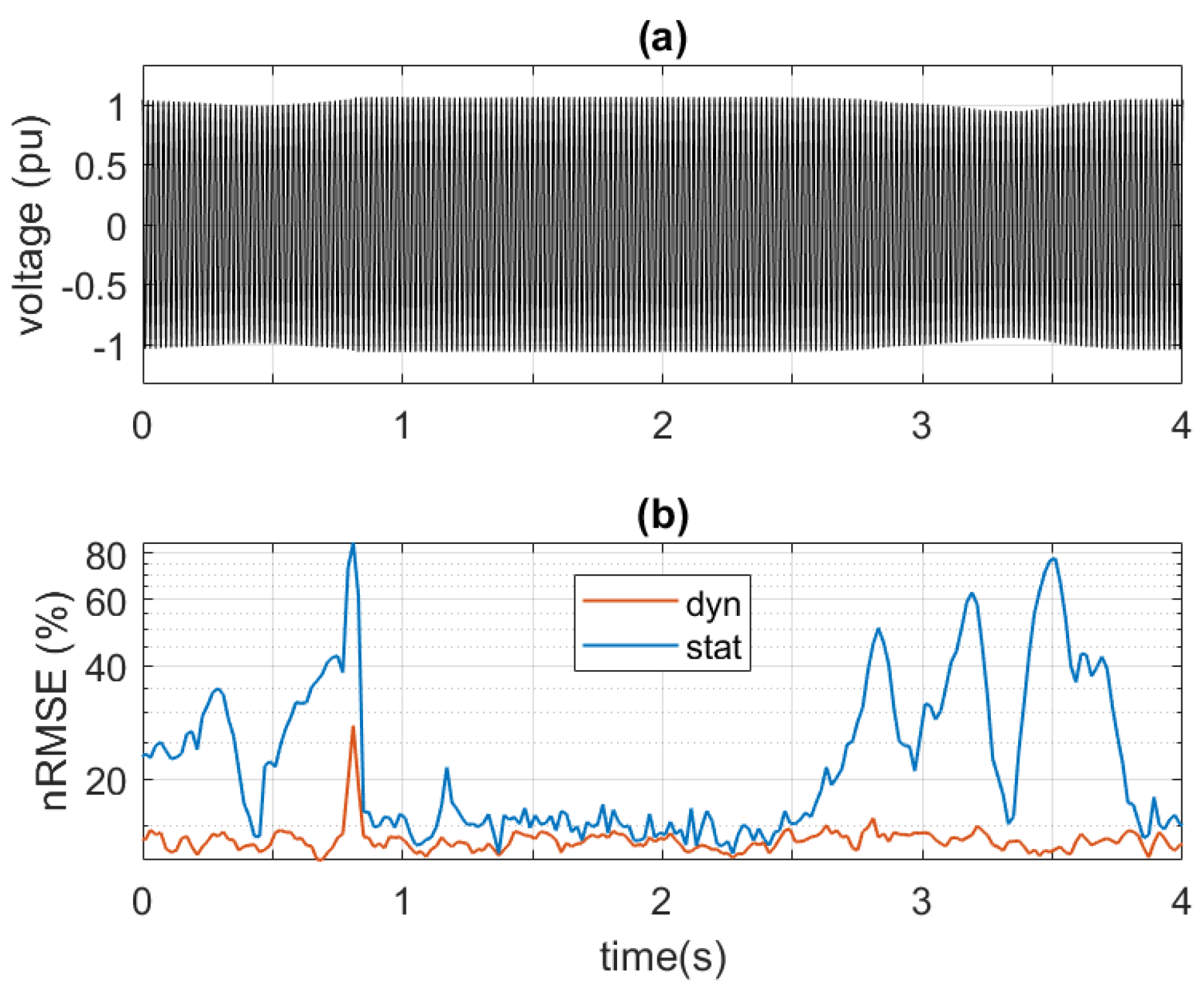
5.2. Feasibility Analysis in Real-World Scenarios

Once characterized the relationship between nRMSE and TVE is in standard test conditions, we can consider a realistic data set. In this way, we investigate whether the nRMSE can be used to detect anomalous or contradictory measurement results, e.g., due to contingencies or due to PMU malfunctions [37].
For this analysis, we consider a simulated data set that reproduces the response to a generation trip in a system, characterized by high shares of renewable energy sources, and software model in [32]). In more detail, the simulated model consists of the well-known IEEE 39-bus system [38], where four synchronous generators are replaced by four wind farms. In order to validate the performance of different ROCOF-based under-frequency load-shedding schemes, the data set reproduces a large contingency event, by synchronously tripping three generation units for an overall loss of 1.5 GW. In this context, Figure 6a presents the voltage profile at bus 26. The contingency occurrence is visible at 200 ms, then nearly 600 ms of a dampened oscillation, then a new contingency at 800 ms.
In Figure 6b,c, we present the static and dynamic nRMSE as computed with different PMU reporting rates: 50 and 100 fps, respectively. In this way, it is possible to evaluate whether the reliability metric not only discriminates between different kinds of transients (e.g., wide-band as at 200 ms, or narrow-band as in the following 600 ms), but also depends on the reporting rate. A higher reporting rate provides a finer time resolution of the metric evolution. Nevertheless, it is interesting to observe how both static and dynamic formulations present consistent results, independently from the adopted reporting rate. In the static case, the nRMSE detects clearly the beginning of the contingency. On the other hand, the dynamic nRMSE allows for discriminating between the two wide-band events and the dampened oscillation in between. In more detail, after the first contingency, the nRMSE exhibits a decreasing trend that reflects the progressive shrinking of the spectral bandwidth of the fundamental component, and, thus, the progressive comeback to an operating condition that can be suitably represented by a dynamic phasor model.

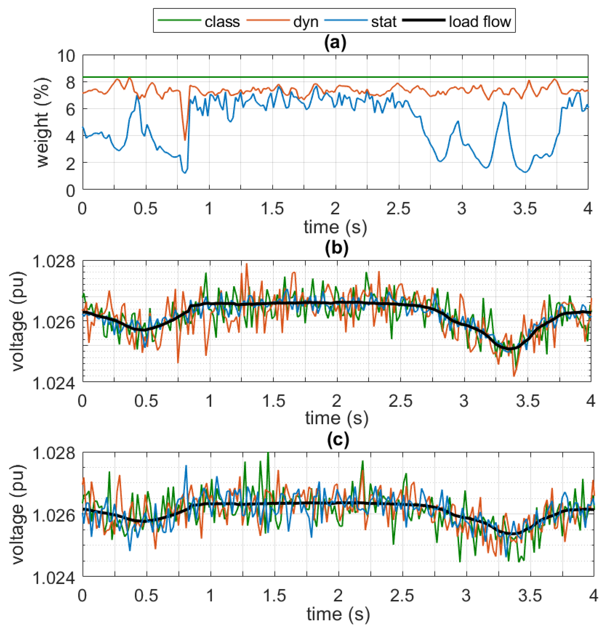
5.3. PMU-Based State Estimation

In modern power systems, PMUs represent the backbone of many monitoring and control applications. Based on the prior knowledge of the network admittance matrix and topology, the PMU-based measurements can be used to retrieve the system states in all the network nodes. The recent literature has investigated several state estimation (SE) methods [39,40,41,42] that can be classified into two main categories [25], namely the static methods as the WLS, and the recursive methods as the DKF.
The SE application of PMU-based measurements yields several advantages. Indeed, PMU-based measurements are linear functions of the state variables, thus leading to a linear state estimation problem, solvable by non-iterative algorithms with reduced computational requirements. Moreover, PMU-based measurements are time-stamped and can be aggregated and time-aligned at a central data collection point. This ensures that every set of measurements given to the SE is composed of measurements taken at the same instant. Finally, the high PMU reporting rate allows for an SE characterized by high refresh rate and low latency, in line with the real-time monitoring requirements of modern power systems.
In the present case, we consider a system whose states are the nodal voltage phasors in all the buses, and the SE is required to infer them from an incomplete set of measurements, namely voltage and current phasors in a subset of buses. Let us assume that the nodal admittance matrix is known exactly a priori. The measurement model is as follows:
m = H s + ε m , ε M N ( 0 , W )
where m and s are the vectors of measurements and states, respectively. Their relationship is defined by the measurement matrix H, while ε M accounts for the measurement uncertainty and is modeled as a purely additive random variable, normally distributed with zero mean and variance defined by the noise covariance matrix W. As first approximation, it is reasonable to assume that the noise affecting each measurement is statistically independent, therefore, W consists of a diagonal matrix.
In the context of DKF, the process model is defined as:
m [ i ] = A m [ i 1 ] + ε P [ i 1 ] ε P N ( 0 , Q [ i 1 ] ) , E ( ε P ε M T ) = 0
where i denotes the reporting index, the process matrix A defines the relationship between current and previous measurements, and ε P accounts for the uncertainty of the process model. Due to the PMU high-reporting rate, it is reasonable to assume that the process matrix corresponds to the identity matrix, i.e., the system evolution is much slower than the measurement update rate. The process noise is modeled as a purely additive random variable, normally distributed with zero mean and a standard deviation that depends on the process noise covariance matrix Q. Similarly, as per W, also Q is defined as a diagonal matrix, i.e., the process noise insisting on each measurement is modeled as a statistically independent random variable. In this regard, it should be noticed that measurement and process noise are assumed to be perfectly uncorrelated.
Based on (9), the PMU measurement process is approximated as an ARIMA model of order (0, 1, 0), also known as the random walk model. The variance of the process noise is initialized to a nominal value, namely 10 8 , and then iteratively updated as the sample variance of a circular buffer with the last ten estimates of the corresponding state.
As mentioned in Section 2, the accuracy of PMU-based measurements is strongly dependent on the employed measurement chain components. Consequently, both static and recursive SE methods allow for associating a weight to each measurement based on some prior information. More specifically, by adjusting the measurement noise covariance matrix W, it is possible to associate different weights to each measurement, in order to reflect the specific PMU reliability. In this sense, it is common practice to use the IT class information to define the most suitable weight for each PMU measurement [43]. It is accordingly assumed that the measurement errors belong to a Gaussian distribution whose variance is derived from the maximum allowed systematic error, as given in Table 1. However, this information is fixed and does not depend on the current system conditions. Therefore in this paper, we investigate whether the application of online performance metrics could be beneficial in terms of state estimation accuracy and robustness.
In Figure 7a, we present the voltage waveform as acquired at node 4 of the IEEE 14 bus network. The effect of the dynamic load model is evident in the amplitude level fluctuations. In Figure 7b, the corresponding nRMSE computed according to the static and dynamic phasor formulations are represented in blue and red, respectively. Once again, the static one is more sensitive to the parameter time variations, whereas the dynamic one exhibits a nearly constant value (mainly dependent on the narrow- and wide-band distortion levels).
Based on the static nRMSE, the PMU-based measurements would be considered highly reliable only in the time interval between t = 1 and t = 2.5 s. Conversely, the dynamic nRMSE keeps a nearly constant value over the considered time span. It is thus reasonable to say that an augmented signal model (that accounts also for higher derivative order terms) is capable of fully representing the system dynamics. On the other hand, it is worth remembering that the quantities involved in the SE are the ones associated with the zero-th-order expansion. Therefore, the dynamic nRMSE may produce a misleading evaluation of the actual PMU reliability.
In the absence of ground-truth reference values, a Load Flow (LF) analysis has been conducted to define the instantaneous value of voltage and current at each reporting time instant. By subtracting them from the simulated waveforms, it is possible to derive the actual measurement noise and verify the assumptions introduced in (7). In this regard, Figure 8 presents the histogram of the measurement noise of the voltage waveform. The red dashed line indicates the best fit with a normal distribution. It is interesting to observe how the distribution is quite consistent with the modeling assumptions. The mean value is equal to zero, and the probability density function is consistent with a normal distribution. Therefore, the combined effect of IT systematic errors, additive measurement noise, and harmonic distortion, can be well approximated by a Gaussian random variable.
In the context of PMU-based state estimation, WLS and DKF represent the most widely used solutions. Indeed, PMU-based state estimation relies on strong assumptions such as the exact knowledge of the network topology and its full observability, but also the fact that measurement errors are uncorrelated with the true state. In such a condition, WLS and DKF represent ideal estimators as they allow to account for the network topology and map the expected measurement uncertainty as an equivalent random variable, normally distributed and with a variance consistent with the expected noise level. The literature has recently proposed several modifications of these two approaches, in order to make them more resilient to possible outliers or bad data. In this sense, a promising solution could be identified in the Least Absolute Value (LAV) estimator, which is less sensitive to leverage measurements. However, from the perspective of the present paper, we preferred to focus on WLS and DKF, where the mapping of the statistical distribution of the expected errors is more straightforward and intuitive.
In this context, we ran the WLS and DKF state estimation with three different configurations of the measurement covariance matrix. As shown in Figure 9a, the noise covariance is set based on the systematic error variances, or equal to the inverse of the nRMSE in its static or dynamic formulation. In this regard, it is interesting to observe how the IT class and the dynamic nRMSE provide comparable values, whereas the static one associates a lower weight to any measurement taken during a non-stationary condition. Figure 9b,c shows the corresponding SE results as compared against the LF reference value for WLS and DKF, respectively. The similarity between the two estimation results descends directly from the adopted process model in (9), which does not yield any significant advantage with respect to the WLS approach.
In terms of estimation errors, it is worth noticing how the dynamic formulation does not produce any improvement with respect to the IT class information, whereas the static one allows for a slight reduction of the noisy oscillations. In a more quantitative way, Figure 10 shows the statistical distribution of the estimation errors as a function of the selected configuration. The box plot refers to the WLS case, but similar results can be obtained in the DKF one. The static nRMSE allows for higher noise rejection in the non-stationary portions of the signals. On the overall considered time interval, though, the RMS error for the three different configurations is quite similar, ranging from 700, 750, and 500 ppm for the class, dynamic, and static configurations, respectively.
Based on the obtained state estimates, it is also possible to verify the assumptions on the measurement noise. In this regard, Figure 11 shows the statistical distribution as inferred from the DKF estimates. The red dashed line indicates the best fit with a normal distribution. In this case, it is worth noticing how the obtained probability density function does not comply with the assumed Gaussian distribution and is strongly affected by the non-compensated effect of the IT systematic errors. In a more quantitative way, the coherence between the measurement noise and its mathematical approximation in the covariance matrix is below 5%. It is thus reasonable to say that the Gaussian assumption is only a limited approximation, and the estimation process cannot be modeled as a linear and predictable process.
This is further proof of the fact that the nRMSE can quantify the uncertainty contributions relative to the PMU acquisition and processing, but cannot account for external contributions, due to other components of the measurement chain. Namely, its application in SE produces a limited performance improvement but represents a promising first effort to associate each measurement value reliability indices that depend not on fixed a priori information, but on the actual operating condition of the instrument.

6. Conclusions

In this paper, we investigated the feasibility of using online performance metrics in PMU-based state estimation. For this analysis, we considered a metric that does not suffer from definitional uncertainty and is characterized by reduced computational requirements. From a metrological point of view, we evaluated its significance and variation range in standard and real-world test conditions, and we compared its confidence interval with other accuracy metrics, whose evaluation is possible only in controlled laboratory conditions.
By means of extensive numerical simulations, we have verified the feasibility of this approach with two well-known state estimators, namely WLS and DKF. The obtained results showed a limited performance improvement, due to the still non-compensated contribution of the other uncertainty components of the measurement chain. Nevertheless, the proposed approach represents a promising first effort to associate to each measurement value reliability indices that depend not on fixed a priori information, but on the actual operating condition of the system and of the instrument.

Future Activities

Based on the obtained results, it is possible to outline some promising research targets and future activities. The continuous improvement of processing capabilities in industrial controllers suggests that modern substations will be equipped with more and more sophisticated devices. It is thus reasonable to assume that the traditional phasor analysis will be soon accompanied by more demanding yet more accurate representations (e.g., the ones based on the Hilbert Transform). In this context, the reliability metric may provide useful information about when to switch to a slower but more accurate stream of information.
Another aspect of interest consists in the proper modeling and validation of the state estimation results. In recent years, more and more studies have investigated the statistical distribution of PMU measurements, either for bad data detection or synthetic dataset generation. In this paper, we prove the strong coherence between reliability metrics and PMU accuracy. It is, therefore, preferable that the statistical investigation of PMU-based application results may include also the reliability metric.

Author Contributions

Conceptualization, G.F. and F.G.-T.; methodology, G.F.; software, G.F.; validation, F.G.-T.; formal analysis, G.F.; resources, F.G.-T.; writing—original draft preparation, G.F.; writing—review and editing, F.G.-T.; supervision, G.F.; project administration, F.G.-T.; funding acquisition, F.G.-T. All authors have read and agreed to the published version of the manuscript.

Funding

This research received no external funding.

Institutional Review Board Statement

Not applicable.

Informed Consent Statement

Not applicable.

Data Availability Statement

The data presented in this study are available on request from the corresponding author. The data are not publicly available due to pending standardization process.

Conflicts of Interest

The authors declare no conflict of interest.

References

  1. Terzija, V.; Valverde, G.; Cai, D.; Regulski, P.; Madani, V.; Fitch, J.; Skok, S.; Begovic, M.M.; Phadke, A. Wide-Area Monitoring, Protection, and Control of Future Electric Power Networks. Proc. IEEE 2011, 99, 80–93. [Google Scholar] [CrossRef]
  2. Rueda Torres, J.; Kumar, N.V.; Rakhshani, E.; Ahmad, Z.; Adabi, E.; Palensky, P.; van der Meijden, M. Dynamic Frequency Support for Low Inertia Power Systems by Renewable Energy Hubs with Fast Active Power Regulation. Electronics 2021, 10, 1651. [Google Scholar] [CrossRef]
  3. Stojković, J.; Stefanov, P. A Novel Approach for the Implementation of Fast Frequency Control in Low-Inertia Power Systems Based on Local Measurements and Provision Costs. Electronics 2022, 11, 1776. [Google Scholar] [CrossRef]
  4. Paolone, M.; Gaunt, T.; Guillaud, X.; Liserre, M.; Meliopoulos, S.; Monti, A.; Van Cutsem, T.; Vittal, V.; Vournas, C. Fundamentals of power systems modelling in the presence of converter-interfaced generation. Electr. Power Syst. Res. 2020, 189, 106811. [Google Scholar] [CrossRef]
  5. Rietveld, G.; Braun, J.P.; Martin, R.; Wright, P.; Heins, W.; Ell, N.; Clarkson, P.; Zisky, N. Measurement Infrastructure to Support the Reliable Operation of Smart Electrical Grids. IEEE Trans. Instrum. Meas. 2015, 64, 1355–1363. [Google Scholar] [CrossRef]
  6. Rouhani, A.; Abur, A. Linear Phasor Estimator Assisted Dynamic State Estimation. IEEE Trans. Smart Grid 2018, 9, 211–219. [Google Scholar] [CrossRef]
  7. Feng, G.; Abur, A. Fault Location Using Wide-Area Measurements and Sparse Estimation. IEEE Trans. Power Syst. 2016, 31, 2938–2945. [Google Scholar] [CrossRef]
  8. Ding, F.; Booth, C.D.; Roscoe, A.J. Peak-Ratio Analysis Method for Enhancement of LOM Protection Using M-Class PMUs. IEEE Trans. Smart Grid 2016, 7, 291–299. [Google Scholar] [CrossRef]
  9. Zhang, Z.; Yang, H.; Yin, X.; Han, J.; Wang, Y.; Chen, G. A Load-Shedding Model Based on Sensitivity Analysis in on-Line Power System Operation Risk Assessment. Energies 2018, 11, 727. [Google Scholar] [CrossRef]
  10. De La Ree, J.; Centeno, V.; Thorp, J.S.; Phadke, A.G. Synchronized Phasor Measurement Applications in Power Systems. IEEE Trans. Smart Grid 2010, 1, 20–27. [Google Scholar] [CrossRef]
  11. Livanos, N.A.I.; Hammal, S.; Giamarelos, N.; Alifragkis, V.; Psomopoulos, C.S.; Zois, E.N. OpenEdgePMU: An Open PMU Architecture with Edge Processing for Future Resilient Smart Grids. Energies 2023, 16, 2756. [Google Scholar] [CrossRef]
  12. 60255-118-1:2018; Measuring Relays and Protection Equipment—Part 118-1: Synchrophasor for Power Systems—Measurements. International Standard; IEC: Geneva, Switzerland, 2018.
  13. IEEE Std C37.242-2013; IEEE Guide for Synchronization, Calibration, Testing, and Installation of Phasor Measurement Units (PMUs) for Power System Protection and Control. IEEE: Piscataway, NJ, USA, 2013; pp. 1–107. [CrossRef]
  14. Tang, Y.H.; Stenbakken, G.N.; Goldstein, A. Calibration of Phasor Measurement Unit at NIST. IEEE Trans. Instrum. Meas. 2013, 62, 1417–1422. [Google Scholar] [CrossRef]
  15. Kirkham, H.; Riepnieks, A. Dealing with non-stationary signals: Definitions, considerations and practical implications. In Proceedings of the 2016 IEEE Power and Energy Society General Meeting (PESGM), Boston, MA, USA, 17–21 July 2016; pp. 1–5. [Google Scholar] [CrossRef]
  16. Qian, C.; Kezunovic, M. A Novel Time-Frequency Analysis for Power System Waveforms Based on “Pseudo-Wavelets”. In Proceedings of the 2018 IEEE/PES Transmission and Distribution Conference and Exposition (T&D), Denver, CO, USA, 16–19 April 2018; pp. 1–9. [Google Scholar] [CrossRef]
  17. Wright, P.S.; Davis, P.N.; Johnstone, K.; Rietveld, G.; Roscoe, A.J. Field Measurement of Frequency and ROCOF in the Presence of Phase Steps. IEEE Trans. Instrum. Meas. 2019, 68, 1688–1695. [Google Scholar] [CrossRef]
  18. Kirkham, H. The measurand: The problem of frequency. In Proceedings of the 2016 IEEE International Instrumentation and Measurement Technology Conference Proceedings, Taipei, Taiwan, 23–26 May 2016; pp. 1–5. [Google Scholar] [CrossRef]
  19. Riepnieks, A.; Kirkham, H. An Introduction to Goodness of Fit for PMU Parameter Estimation. IEEE Trans. Power Deliv. 2017, 32, 2238–2245. [Google Scholar] [CrossRef]
  20. Frigo, G.; Colangelo, D.; Derviškadić, A.; Pignati, M.; Narduzzi, C.; Paolone, M. Definition of Accurate Reference Synchrophasors for Static and Dynamic Characterization of PMUs. IEEE Trans. Instrum. Meas. 2017, 66, 2233–2246. [Google Scholar] [CrossRef]
  21. Yousof, H.M.; Goual, H.; Emam, W.; Tashkandy, Y.; Alizadeh, M.; Ali, M.M.; Ibrahim, M. An Alternative Model for Describing the Reliability Data: Applications, Assessment, and Goodness-of-Fit Validation Testing. Mathematics 2023, 11, 1308. [Google Scholar] [CrossRef]
  22. Frigo, G.; Grasso Toro, F. On-line performance assessment for improved sensor data aggregation in power system metrology. Meas. Sens. 2021, 18, 100186. [Google Scholar] [CrossRef]
  23. Rahmatian, M.; Chen, Y.C.; Dunford, W.G.; Rahmatian, F. Incorporating Goodness-of-Fit Metrics to Improve Synchrophasor-Based Fault Location. IEEE Trans. Power Deliv. 2018, 33, 1944–1953. [Google Scholar] [CrossRef]
  24. Frigo, G.; Toro, F.G. Metrological Significance and Reliability of On-Line Performance Metrics in PMU-based WLS State Estimation. In Proceedings of the 2022 International Conference on Smart Grid Synchronized Measurements and Analytics (SGSMA), Split, Croatia, 24–26 May 2022; pp. 1–6. [Google Scholar] [CrossRef]
  25. Paolone, M.; Le Boudec, J.Y.; Sarri, S.; Zanni, L. Static and recursive PMU-based state estimation processes for transmission and distribution power grids. In Advanced Techniques for Power System Modelling, Control and Stability Analysis; IET: London, UK, 2015; pp. 189–239. [Google Scholar]
  26. Fotopoulou, M.; Petridis, S.; Karachalios, I.; Rakopoulos, D. A Review on Distribution System State Estimation Algorithms. Appl. Sci. 2022, 12, 11073. [Google Scholar] [CrossRef]
  27. Illinois Center for a Smarter Electric Grid. IEEE 14-Bus System. 2021. Available online: https://icseg.iti.illinois.edu/ieee-14-bus-system/ (accessed on 9 October 2021).
  28. Frigo, G.; Derviškadić, A.; Zuo, Y.; Bach, A.; Paolone, M. Taylor-Fourier PMU on a Real-Time Simulator: Design, Implementation and Characterization. In Proceedings of the 2019 IEEE Milan PowerTech, Milan, Italy, 23–27 June 2019; pp. 1–6. [Google Scholar] [CrossRef]
  29. 62586-2:2017+AMD1:2021; Power Quality Measurement in Power Supply Systems—Part 2: Functional Tests and Uncertainty Requirements. International Standard; IEC: Geneva, Switzerland, 2021.
  30. Roscoe, A.J.; Blair, S.M.; Dickerson, B.; Rietveld, G. Dealing with Front-End White Noise on Differentiated Measurements Such as Frequency and ROCOF in Power Systems. IEEE Trans. Instrum. Meas. 2018, 67, 2579–2591. [Google Scholar] [CrossRef]
  31. Arefin, A.A.; Baba, M.; Singh, N.S.S.; Nor, N.B.M.; Sheikh, M.A.; Kannan, R.; Abro, G.E.M.; Mathur, N. Review of the Techniques of the Data Analytics and Islanding Detection of Distribution Systems Using Phasor Measurement Unit Data. Electronics 2022, 11, 2967. [Google Scholar] [CrossRef]
  32. Zuo, Y.; Derviskadic, A.; Frigo, G.; Paolone, M. IEEE-39-Bus-4WG-Power-System. 2018. Available online: https://github.com/DESL-EPFL/IEEE-39-bus-4WG-power-system (accessed on 29 August 2022).
  33. Mingotti, A.; Betti, C.; Peretto, L.; Tinarelli, R. Simplified and Low-Cost Characterization of Medium-Voltage Low-Power Voltage Transformers in the Power Quality Frequency Range. Sensors 2022, 22, 2274. [Google Scholar] [CrossRef] [PubMed]
  34. Pegoraro, P.A.; Castello, P.; Muscas, C.; Brady, K.; von Meier, A. Handling Instrument Transformers and PMU Errors for the Estimation of Line Parameters in Distribution Grids. In Proceedings of the 2017 IEEE International Workshop on Applied Measurements for Power Systems (AMPS), Liverpool, UK, 20–22 September 2017; pp. 1–6. [Google Scholar] [CrossRef]
  35. Price, W.W. Load representation for dynamic performance analysis (of power systems). IEEE Trans. Power Syst. 1993, 8, 472–482. [Google Scholar] [CrossRef]
  36. Ferrero, R.; Pegoraro, P.A.; Toscani, S. Impact of Capacitor Voltage Transformers on Phasor Measurement Units Dynamic Performance. In Proceedings of the 2018 IEEE 9th International Workshop on Applied Measurements for Power Systems (AMPS), Bologna, Italy, 26–28 September 2018; pp. 1–6. [Google Scholar] [CrossRef]
  37. Kummerow, A.; Monsalve, C.; Brosinsky, C.; Nicolai, S.; Westermann, D. A Novel Framework for Synchrophasor Based Online Recognition and Efficient Post-Mortem Analysis of Disturbances in Power Systems. Appl. Sci. 2020, 10, 5209. [Google Scholar] [CrossRef]
  38. Pes, I. Benchmark Systems for Small-Signal Stability Analysis and Control; Technical report; IEEE: Austin, TX, USA, 2015. [Google Scholar]
  39. Gomez-Exposito, A.; Abur, A.; de la Villa Jaen, A.; Gomez-Quiles, C. A Multilevel State Estimation Paradigm for Smart Grids. Proc. IEEE 2011, 99, 952–976. [Google Scholar] [CrossRef]
  40. Muscas, C.; Pau, M.; Pegoraro, P.A.; Sulis, S. Uncertainty of Voltage Profile in PMU-Based Distribution System State Estimation. IEEE Trans. Instrum. Meas. 2016, 65, 988–998. [Google Scholar] [CrossRef]
  41. Kettner, A.M.; Paolone, M. Sequential Discrete Kalman Filter for Real-Time State Estimation in Power Distribution Systems: Theory and Implementation. IEEE Trans. Instrum. Meas. 2017, 66, 2358–2370. [Google Scholar] [CrossRef]
  42. Zhao, J.; Gómez-Expósito, A.; Netto, M.; Mili, L.; Abur, A.; Terzija, V.; Kamwa, I.; Pal, B.; Singh, A.K.; Qi, J.; et al. Power System Dynamic State Estimation: Motivations, Definitions, Methodologies, and Future Work. IEEE Trans. Power Syst. 2019, 34, 3188–3198. [Google Scholar] [CrossRef]
  43. Asprou, M.; Kyriakides, E.; Albu, M. The Effect of Variable Weights in a WLS State Estimator Considering Instrument Transformer Uncertainties. IEEE Trans. Instrum. Meas. 2014, 63, 1484–1495. [Google Scholar] [CrossRef]
Figure 1. Classifications of the uncertainty contributions inherent in a PMU-based measurement system are intrinsic, measurement, and overall uncertainty.
Applsci 13 11670 g001
Figure 2. Network diagram of the IEEE 14-bus test case.
Applsci 13 11670 g002
Figure 3. Diagram of the simulated dynamic EPRI LOADSYN model.
Applsci 13 11670 g003
Figure 4. Steady-state conditions: comparison of nRMSE as computed on static and dynamic phasor representation (a) and corresponding TVE (b) as a function of the selected voltage transformer class.
Applsci 13 11670 g004
Figure 5. Phase modulation: comparison of nRMSE as computed on static and dynamic phasor representation (a) and corresponding TVE (b) as a function of the selected voltage transformer class.
Applsci 13 11670 g005
Figure 6. In (a), voltage profile of a signal affected by contingencies in reduced inertia conditions. In (b,c), the static (blue) and dynamic nRMSE (red) as computed with a PMU reporting rate of 50 and 100 fps, respectively.
Applsci 13 11670 g006
Figure 7. In (a), voltage signal as acquired by the PMU at node 4. In (b), nRMSE is measured based on static (blue) and dynamic (red) phasor representation.
Applsci 13 11670 g007
Figure 8. Statistical distribution of measurement noise as derived from simulated voltage signal and LF-based ground-truth values. The red dashed line represents the best fit with a Gaussian distribution.
Applsci 13 11670 g008
Figure 9. In (a), measurement weights are based on VT class (green), static (blue), and dynamic (red) nRMSE. In (b,c), WLS and DKF estimates of voltage real part in node 4 against the load flow (black) reference values.
Applsci 13 11670 g009
Figure 10. Statistical distribution of the estimation errors in the WLS case as a function of the weight configuration.
Applsci 13 11670 g010
Figure 11. Statistical distribution of measurement noise as inferred from DKF estimates. The red dashed line represents the best fit with a Gaussian distribution.
Applsci 13 11670 g011
Table 1. Instrument Transformer Classes.
TypeClass Δ ε (%) Δ ε (mrad)Nodes
VT0.10.11.451, 2, 5, 7, 8
0.50.55.823, 4, 6, 9, 10–14
CT0.20.22.911, 2, 5, 7, 8
0.50.58.733, 4, 6, 9, 10–14
Table 2. TVE vs. nRMSE—Correlation Analysis.
TestModelCorr (%)p-Value (%)Conf (%)
VT 0.10.50.10.50.10.5
SSstat96.3293.200.010.013.895.43
dyn13.821.7317.7189.4439.1639.88
PMstat36.2333.790.031.2814.8419.83
dyn8.645.8739.9956.7839.6039.76
Disclaimer/Publisher’s Note: The statements, opinions and data contained in all publications are solely those of the individual author(s) and contributor(s) and not of MDPI and/or the editor(s). MDPI and/or the editor(s) disclaim responsibility for any injury to people or property resulting from any ideas, methods, instructions or products referred to in the content.

