Performance Analysis of Interval Type-2 Fuzzy $\overline{\mathbf{X}}$ and R Control Charts

Abstract

Statistical process control (SPC) is one of the most powerful techniques for improving quality, as it is able to detect special causes of problems in processes, products and services with a remarkable degree of accuracy. Among SPC tools, $\overline{\mathrm{X}}$ and R control charts are widely employed in process monitoring. However, scenarios involving vague, imprecise and even subjective data require a type-2 fuzzy set approach. Thus, $\overline{\mathrm{X}}$ and R control charts should be coupled with interval type-2 triangular fuzzy numbers (IT2TFN) in order to add further information to traditional control charts. This paper proposes a performance analysis of IT2TFN and $\overline{\mathrm{X}}$ and R control charts by means of average run length (ARL), standard deviation of the run length (SDRL) and RL percentile. Computer simulations were carried out considering 10,000 runs to obtain ARL, SDRL and the 5th, 25th, 50th, 75th and 95th RL percentiles. Simulation results reveal that the proposed control charts increased fault detection capability (speed of response) and slightly reduced the number of false alarms in processes under control. Moreover, it was observed that, in addition to superior performance, IT2TFN $\overline{\mathrm{X}}$-R control charts proved to be more robust and flexible when compared to traditional control charts.

1. Introduction

Among statistical process control (SPC) tools, control charts are by far the most widely used method due to the simplicity of understanding them, while at the same time being efficient in detecting defects in production processes [1].

There are two types of control charts: variable or attribute control charts. According to [2], such classification is made according to the type of data being monitored. In variable control charts, the degree of data precision (usually defined by the number of decimal places) and continuous data, such as length, height, mass, time, among others, can be measured. For attribute control charts, data may or may not have some attributes, such as number of nonconforming items or number of nonconformities per lot, thus requiring the use of discrete variables that are countable.

When human judgments and subjectivity significantly affect the definition of quality characteristics, traditional control charts should be used. In such a case, the theory of fuzzy sets developed by [3] should be used instead, since it enhances the flexibility of control charts and adds further information about process details, in addition to its performance improvement capability [4].

In scenarios containing several sources of uncertainty regarding the data under analysis, the type-2 fuzzy set approach proposed by [5] should be used, which was mathematically formulated by [6].

Measurement error is a concept related to the difference between a measured value and the reference value of a measurand. As measurement errors cannot be fully corrected, there will always be a portion of doubt associated with measurements, which is represented by uncertainty [7]. The theory of type-2 fuzzy sets is applied in order to model this uncertainty.

Type-1 fuzzy logic makes use of uncertainties related to the meanings of words through precise membership functions. Such membership functions, when well defined, are capable of eliminating uncertainties arising from the meanings of words. A membership function of type-2 fuzzy sets, on the other hand, measures uncertainty through the so-called footprint of uncertainty (FOU), which allows working on a higher level of uncertainty. Therefore, if type-2 fuzzy pertinence functions are well defined, type-2 uncertainties are also eliminated and data are restored to type-1 fuzzy numbers [6].

Regarding the performance of fuzzy control charts, [8] presented type-1 fuzzy $\overline{\mathrm{X}}$-R control charts for monitoring the mean and range of univariate processes. Through a performance analysis, the authors observed that fuzzy control charts achieved higher efficiency in detecting special causes compared to traditional control charts.

$\overline{\mathrm{X}}$ and R control charts through the approach presented by [9] allowed implementing exponentially weighted moving average (EWMA) control charts using fuzzy numbers to monitor the average and range of processes. A performance analysis of their proposed control chart through ARL proved to be more efficient than traditional control charts. Furthermore, future research on the use of other performance metrics such as standard deviation of the run length (SDRL) and median of the run length (MDRL) has been suggested.

Therefore, this paper proposes a performance analysis of $\overline{X}$-R control charts under the use of interval type-2 fuzzy sets in univariate processes through the average run length (ARL), SDRL and percentile of RL. Equations for control limits using triangular type-2 fuzzy numbers will be presented, and simulations were performed to show the values of ARL, SDRL and percentile of RL as functions of the variation in parameters δ (shift), λ (disturbance) and the FOU. Finally, an illustrative example will be presented.

Although there are other control chart models using fuzzy set theory, the $\overline{\mathrm{X}}$ and R control charts are most applied to industrial processes due to their simplicity of implementation and their comprehensive application in variable monitoring of different process types.

This paper is organized as follows: Section 2 introduces the concepts of type-2 fuzzy sets, interval type-2 triangular fuzzy number (IT2TFN) operations, the defuzzification method and footprint of uncertainty. Section 3 presents the proposed interval type-2 fuzzy $\overline{\mathrm{X}}$-R control charts. Section 4 shows the ARL, SDRL and RL percentile performance measurements together with variables making up in-control and out-of-control conditions. Section 5 contains details about the performance analysis of proposed fuzzy control charts. Finally, Section 6 draws conclusions and offers suggestions for future research.

2. Interval Type-2 Fuzzy Sets

According to [10], a type-2 fuzzy set, denoted by $\tilde{A}$, can be characterized by the membership function ${\mu }_{\tilde{A}}=\left(x,u\right)$, where x $\in$ X and u $\in$ Jx $\subseteq$ [0, 1].

Mathematically, it is represented as:

$$\tilde{\mathrm{A}}=\left\{\left(\left(\mathrm{x},\mathrm{u}\right),{\mathsf{\mu }}_{\tilde{\mathrm{A}}}\left(\mathrm{x},\mathrm{u}\right)\right)|\forall \mathrm{x}\in \mathrm{X},\forall \mathrm{u}\in {\mathrm{J}}_{\mathrm{x}}\subseteq \left[0, 1\right]\right\}$$

(1)

where $0 \le {\mu }_{\tilde{A}} \le 1$.

According to this work, an interval type-2 triangular fuzzy number (IT2TFN) can be illustrated as shown in Figure 1.

Although the fuzzy set theory proposed by [3] offers great advantages, classical fuzzy sets are unable to model uncertainty through clear definitions of pertinence functions at times. Thus, type-2 fuzzy sets should be used as they successfully improve the quality of uncertainty modeling. It is also known that pertinence functions of classical fuzzy sets are bidimensional, while those of type-2 fuzzy sets are three-dimensional, therefore type-2 fuzzy sets can accurately represent uncertainty and reduce its undesirable/negative effects [11].

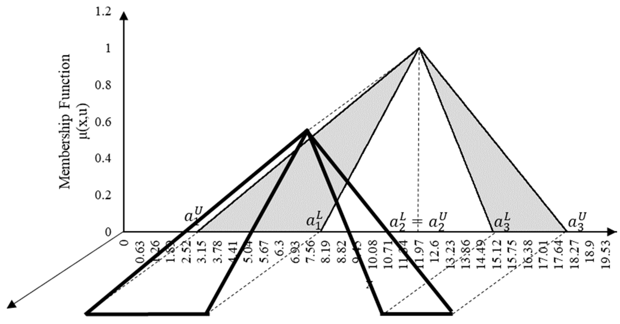
2.1. Interval Type-2 Triangular Fuzzy Sets

An interval type-2 fuzzy set $\tilde{\mathrm{A}}$ is represented by a lower membership function (LMF) ${\tilde{A}}^L$ and an upper membership function (UMF)${ \tilde{\mathrm{A}}}^{\mathrm{U}}$, where$\tilde{\mathrm{A}}={ \tilde{\mathrm{A}}}^{\mathrm{L}},{ \tilde{\mathrm{A}}}^{\mathrm{U}}$. In particular, when triangular pertinence functions are used, it is illustrated as in Figure 2, where ${\tilde{A}}^L=\left(a_{i1}^L,a_{i2}^L,a_{i3}^L; H\left({\tilde{A}}^L\right)\right)$, ${\tilde{A}}^U=\left(a_{i1}^U,a_{i2}^U,a_{i3}^U; H\left({\tilde{A}}^U\right)\right)$, $(a_{i1}^L,a_{i2}^L,a_{i3}^L)$ and $(a_{i1}^U,a_{i2}^U,a_{i3}^U)$ denote three key points of LMF and UMF, and${ \tilde{\mathrm{A}}}^{\mathrm{L}}$ and${ \tilde{\mathrm{A}}}^{\mathrm{U}}$, where $a_1^U\le a_1^L$, $a_3^U\le a_3^L$, $0< \mathrm{H} \left({ \tilde{\mathrm{A}}}^{\mathrm{L}}\right)\le \mathrm{H}\left({ \tilde{\mathrm{A}}}^{\mathrm{U}}\right)=1$, denote the highest membership function values.

Upper membership and lower membership functions are described according to Equations (2) and (3), respectively:

$${\mathsf{\mu }}_{\tilde{\mathrm{A}}}^{\mathrm{U}}=\left\{\begin{array}{c}\frac{\mathrm{x}-a_1^{\mathrm{U}}}{a_2^{\mathrm{U}}-a_1^{\mathrm{U}}};\mathrm{if} a_1^{\mathrm{U}} \le \mathrm{x} \le a_2^{\mathrm{U}}\\ \frac{a_3^{\mathrm{U}}-\mathrm{x}}{a_3^{\mathrm{U}}-a_2^{\mathrm{U}}};\mathrm{if} a_2^{\mathrm{U}} \le \mathrm{x} \le a_3^{\mathrm{U}}\end{array}\right.$$

(2)

$${\mathsf{\mu }}_{ \tilde{\mathrm{A}}}^{\mathrm{L}}=\left\{\begin{array}{c}\frac{\mathrm{x}-a_1^{\mathrm{L}}}{a_2^{\mathrm{L}}-a_1^{\mathrm{L}}};\mathrm{if} a_1^{\mathrm{L}} \le \mathrm{x} \le a_2^{\mathrm{L}}\\ \frac{a_3^{\mathrm{L}}-\mathrm{x}}{a_3^{\mathrm{L}}-a_2^{\mathrm{L}}};\mathrm{if} a_2^{\mathrm{L}} \le \mathrm{x} \le a_3^{\mathrm{L}}\end{array}\right.$$

(3)

The closer the shapes of ${ \tilde{\mathrm{A}}}^{\mathrm{L}}$ and ${ \tilde{\mathrm{A}}}^{\mathrm{U}}$ are, the less uncertain information contained in $\tilde{\mathrm{A}}$ obviously is. When ${ \tilde{\mathrm{A}}}^{\mathrm{L}}$ coincides with ${ \tilde{\mathrm{A}}}^{\mathrm{U}}$, the interval type-2 fuzzy set becomes a type-1 fuzzy set [12].

In order to simplify the model, the central IT2TFN value $a_2^U=a_2^L$ is considered, as it defines the singleton of an interval type-2 triangular fuzzy number, but height $H\left({\tilde{A}}^U\right)$ of the upper membership function coincides with height $\mathrm{H}\left({ \tilde{\mathrm{A}}}^{\mathrm{L}}\right)$ of the lower membership function. Particularly where $a_2^U=a_2^L$ and $H\left({\tilde{A}}^U\right)=H\left({\tilde{A}}^L\right)$, the so-called perfect interval type-2 triangular fuzzy number (PI2TFN) is obtained [13].

The arithmetic operations of addition, subtraction and multiplication, respectively, are used in $\overline{\mathrm{X}}$-R control charts for IT2TFN, which are given by Equations (4)–(6) according to [14]:

$${ \tilde{\mathrm{A}}}_1+{ \tilde{\mathrm{A}}}_2=\left(\begin{array}{c}\left(a_{11}^{\mathrm{U}}+a_{21}^{\mathrm{U}},a_{12}^{\mathrm{U}}+a_{22}^{\mathrm{U}},a_{13}^{\mathrm{U}}+a_{23}^{\mathrm{U}};\min \left(\mathrm{H}({ \tilde{\mathrm{A}}}_1^{\mathrm{U}}\right),\left(\mathrm{H}({ \tilde{\mathrm{A}}}_2^{\mathrm{U}}\right) \right),\\ \left(a_{11}^{\mathrm{L}}+a_{21}^{\mathrm{L}},a_{12}^{\mathrm{L}}+a_{22}^{\mathrm{L}},a_{13}^{\mathrm{L}}+a_{23}^{\mathrm{L}};\min \left(\mathrm{H}({ \tilde{\mathrm{A}}}_1^{\mathrm{L}}\right),\left(\mathrm{H}({ \tilde{\mathrm{A}}}_2^{\mathrm{L}}\right) \right)\end{array}\right)$$

(4)

$${ \tilde{\mathrm{A}}}_1-{ \tilde{\mathrm{A}}}_2=\left(\begin{array}{c}\left(a_{11}^{\mathrm{U}}-a_{23}^{\mathrm{U}},a_{12}^{\mathrm{U}}-a_{22}^{\mathrm{U}},a_{13}^{\mathrm{U}}-a_{21}^{\mathrm{U}};\min \left(\mathrm{H}({ \tilde{\mathrm{A}}}_1^{\mathrm{U}}\right),\left(\mathrm{H}({ \tilde{\mathrm{A}}}_2^{\mathrm{U}}\right) \right),\\ \left(a_{11}^{\mathrm{L}}-a_{23}^{\mathrm{L}},a_{12}^{\mathrm{L}}-a_{22}^{\mathrm{L}},a_{13}^{\mathrm{L}}-a_{21}^{\mathrm{L}};\min \left(\mathrm{H}({ \tilde{\mathrm{A}}}_1^{\mathrm{L}}\right),\left(\mathrm{H}({ \tilde{\mathrm{A}}}_2^{\mathrm{L}}\right) \right)\end{array}\right)$$

(5)

$${\mathrm{kx} \tilde{\mathrm{A}}}_{\mathrm{i}}=\left(\begin{array}{c}\left(\mathrm{kx}{a}_{\mathrm{i}1}^{\mathrm{U}},\mathrm{kx}{a}_{\mathrm{i}2}^{\mathrm{U}}, \mathrm{kx}{a}_{\mathrm{i}3}^{\mathrm{U}};\min \left(\mathrm{H}({ \tilde{\mathrm{A}}}_{\mathrm{i}}^{\mathrm{U}}\right) \right),\\ \left(\mathrm{kx}{a}_{11}^{\mathrm{L}}, \mathrm{kx}{a}_{12}^{\mathrm{L}},\mathrm{kx}{a}_{13}^L;\min \left(\mathrm{H}({ \tilde{\mathrm{A}}}_{\mathrm{i}}^{\mathrm{L}}\right) \right)\end{array}\right)$$

(6)

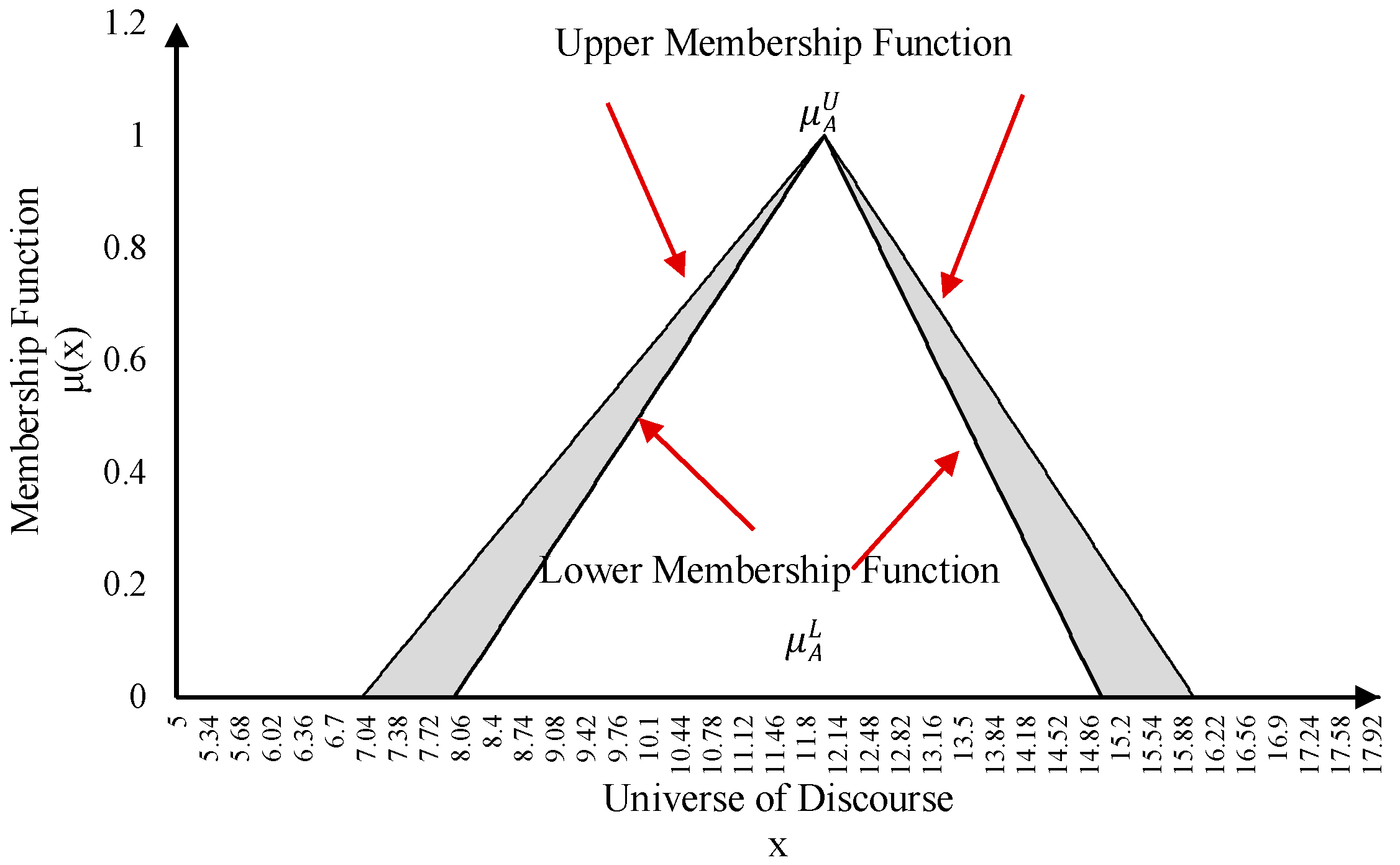
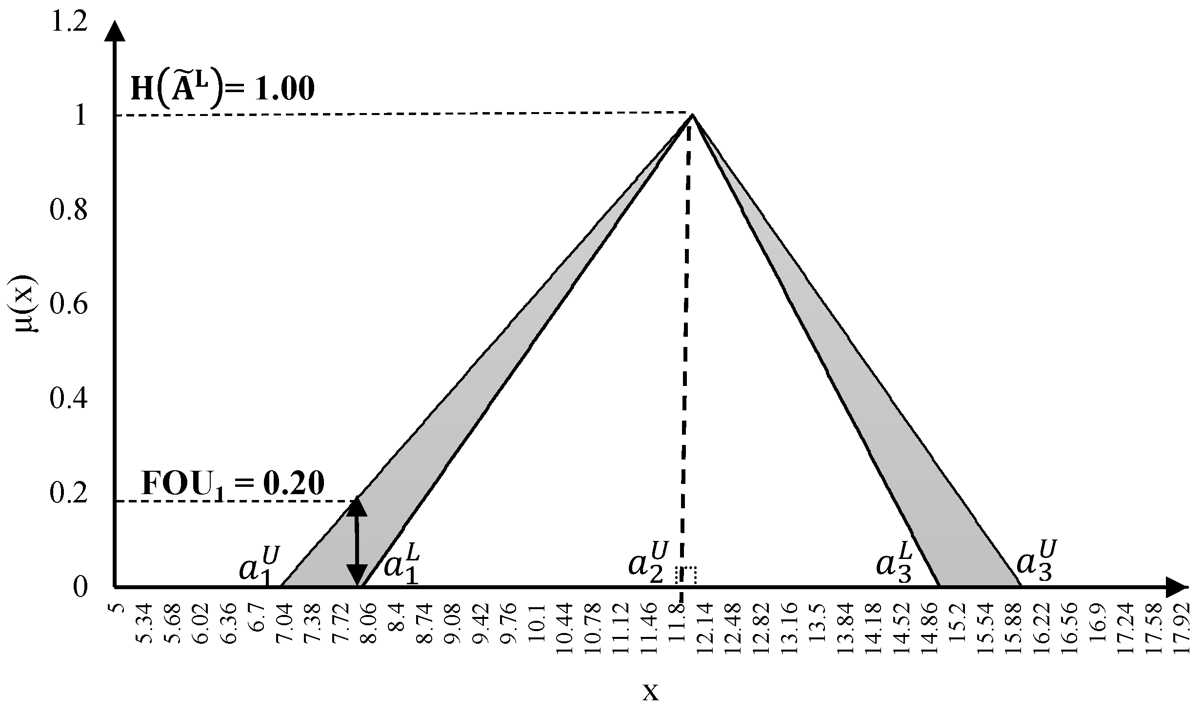
2.2. Footprint of Uncertainty and Membership Functions

According to [12], the uncertainty of primary pertinence functions in type-2 fuzzy sets is represented by the footprint of uncertainty (FOU). If this aspect is not present, the type-2 fuzzy set in question becomes an ordinary fuzzy set. Figure 3 illustrates the FOU of triangular interval type-2 fuzzy set. Its height should be consistent with the type of problem under analysis as well as with the desired degree of uncertainty [10].

The FOU provides an additional degree of freedom for a type-2 fuzzy set so as to directly handle system uncertainties. Thus, it is worth mentioning that FOU is able to model uncertainties in systems making use of type-2 fuzzy sets [15,16]. The FOU of an IT2TFN set is illustrated by Figure 3.

Concerning the most usual FOU values, [17] demonstrate the analytical structure variation in values of FOU (θ) ranging from 0 to 0.5. In order to discuss other values of FOU, [18] reported the differences between FOU values and used PI controllers through interval type-2 fuzzy numbers. It is worth mentioning that the value of the FOU depends on the type of application and what is to be controlled.

Table 1. FOU values according to objectives of a control system. Adapted from [18].

Target	FOU Values (θ)	FOU Relationship
Faster response	0.00 < θ1 = θ2 = θ ≤ 0.50	They should be equal and small
Response with lower or no overshoot	0.50 ≤ θ1 = θ2 = θ < 1.00	They should be equal and larg
Smaller overshoot and faster response	0.30 ≤ θ1 = θ2 = θ < 0.90	They should be equal and medium sized

summarizes the objectives according to FOU values.

Thus, it can be observed how FOU can make systems more flexible, in addition to allowing an increase in the speed of response and/or stabilize data in order to avoid decision-making errors.

With regard to SPC, [19] describe that the aim of process monitoring is to detect shifts in statistical parameters. In this case, when interval type-2 fuzzy sets are used, the value of the FOU can increase this capacity for detecting statistical parameters, when greater response speed is required (rigorous inspection), or decrease the capacity for detecting these parameters, reducing unnecessary stops on the production line (moderate inspection).

3. Interval Type-2 Fuzzy $\overline{X}$ and R Control Charts

Regarding a type of quality characteristic able to be expressed as a measure, it is common to monitor both the mean value and variability. The $\overline{\mathrm{X}}$ control chart is widely used to monitor mean and variability of a process which can be controlled by an R chart [20].

Fuzzy control charts must be used in the following cases: when statistical data under consideration are uncertain or vague or when available data about the process are incomplete or include human subjectivity [21].

Regarding the characteristics of the fuzzy set, [22] proposed $\overline{\mathrm{X}}$ and R and $\overline{\mathrm{X}}$ and S control chart models using triangular fuzzy numbers. The alpha-cut midrange transformation technique was used for data defuzzification, and representative fuzzy values were found using control charts.

Subsequently, [14] proposed $\overline{\mathrm{X}}$ and R control charts using interval type-2 trapezoidal fuzzy numbers (IT2TraFN). Adapting equations to triangular fuzzy numbers, parameters $\overline{X}$ and R to be plotted can be more clearly understood by (7) and (8):

$${ \overline{\mathrm{x}}}_{\mathrm{IT}2\mathrm{TFN}}=\left(\frac{{{\displaystyle \sum }}_{\mathrm{i}=1}^{\mathrm{n}}{\mathrm{x}}_1^{\mathrm{U}}}{\mathrm{n}}, \frac{{{\displaystyle \sum }}_{\mathrm{i}=1}^{\mathrm{n}}{\mathrm{x}}_1^{\mathrm{L}}}{\mathrm{n}}, \frac{{{\displaystyle \sum }}_{\mathrm{i}=1}^{\mathrm{n}}{\mathrm{x}}_2^{\mathrm{U}}}{\mathrm{n}}, \frac{{{\displaystyle \sum }}_{\mathrm{i}=1}^{\mathrm{n}}{\mathrm{x}}_3^{\mathrm{L}}}{\mathrm{n}}, \frac{{{\displaystyle \sum }}_{\mathrm{i}=1}^{\mathrm{n}}{\mathrm{x}}_3^{\mathrm{U}}}{\mathrm{n}}\right)$$

(7)

$${\mathrm{R}}_{\mathrm{IT}2\mathrm{TFN}}=\left(\max {\mathrm{x}}_1^{\mathrm{U}}-\min {\mathrm{x}}_3^{\mathrm{U}}, \max {\mathrm{x}}_1^{\mathrm{L}}-\min {\mathrm{x}}_3^{\mathrm{L}}, \max {\mathrm{x}}_2^{\mathrm{U}}-\min {\mathrm{x}}_2^{\mathrm{U}}, \max {\mathrm{x}}_3^{\mathrm{L}}-\min {\mathrm{x}}_1^{\mathrm{L}}, \max {\mathrm{x}}_3^{\mathrm{U}}-\min {\mathrm{x}}_1^{\mathrm{U}}\right)$$

(8)

where variable x is an interval type-2 triangular fuzzy number in the format $\left({\mathrm{x}}_{\mathrm{i}1}^{\mathrm{U}},{ \mathrm{x}}_{\mathrm{i}1}^{\mathrm{L}},{ \mathrm{x}}_{\mathrm{i}2}^{\mathrm{L}}={\mathrm{x}}_{\mathrm{i}2}^{\mathrm{U}},{ \mathrm{x}}_{\mathrm{i}3}^{\mathrm{L}},{\mathrm{x}}_{\mathrm{i}3}^{\mathrm{U}}\right)$ and n is the sample size.

The average of sample means and sample mean amplitude for m samples can be calculated as in Equations (9) and (10):

$${\stackrel{=}{\mathrm{x}}}_{\mathrm{IT}2\mathrm{TFN}}=\left(\frac{{{\displaystyle \sum }}_{\mathrm{i}=1}^{\mathrm{n}}{ \overline{\mathrm{x}}}_1^{\mathrm{U}}}{\mathrm{m}}, \frac{{{\displaystyle \sum }}_{\mathrm{i}=1}^{\mathrm{n}}{ \overline{\mathrm{x}}}_1^{\mathrm{L}}}{\mathrm{m}}, \frac{{{\displaystyle \sum }}_{\mathrm{i}=1}^{\mathrm{n}}{ \overline{\mathrm{x}}}_2^{\mathrm{U}}}{\mathrm{m}}, \frac{{{\displaystyle \sum }}_{\mathrm{i}=1}^{\mathrm{n}}{ \overline{\mathrm{x}}}_3^{\mathrm{L}}}{\mathrm{m}}, \frac{{{\displaystyle \sum }}_{\mathrm{i}=1}^{\mathrm{n}}{ \overline{\mathrm{x}}}_3^{\mathrm{U}}}{\mathrm{m}}\right)$$

(9)

$${ \overline{\mathrm{R}}}_{\mathrm{IT}2\mathrm{TFN}}=\left(\frac{{{\displaystyle \sum }}_{\mathrm{i}=1}^{\mathrm{n}}{\mathrm{R}}_1^{\mathrm{U}}}{\mathrm{m}}, \frac{{{\displaystyle \sum }}_{\mathrm{i}=1}^{\mathrm{n}}{\mathrm{R}}_1^{\mathrm{L}}}{\mathrm{m}}, \frac{{{\displaystyle \sum }}_{\mathrm{i}=1}^{\mathrm{n}}{\mathrm{R}}_2^{\mathrm{U}}}{\mathrm{m}}, \frac{{{\displaystyle \sum }}_{\mathrm{i}=1}^{\mathrm{n}}{\mathrm{R}}_3^{\mathrm{L}}}{\mathrm{m}}, \frac{{{\displaystyle \sum }}_{\mathrm{i}=1}^{\mathrm{n}}{\mathrm{R}}_3^{\mathrm{U}}}{\mathrm{m}}\right)$$

(10)

Upper (UCL) and lower control limits (LCL), and the center line (CL) for the $\overline{\mathrm{X}}$ control chart can be obtained from Equations (11)–(13):

$${\mathrm{UCL}}_{\mathrm{IT}2\mathrm{TFN}}=\left(\begin{array}{c}{\stackrel{=}{\mathrm{x}}}_1^{\mathrm{U}}+{\mathrm{A}}_2{ \overline{\mathrm{R}}}_1^{\mathrm{U}}, {\stackrel{=}{\mathrm{x}}}_1^{\mathrm{L}}+{\mathrm{A}}_2{ \overline{\mathrm{R}}}_1^{\mathrm{L}}, {\stackrel{=}{\mathrm{x}}}_2^{\mathrm{U}}+{\mathrm{A}}_2{ \overline{\mathrm{R}}}_2^{\mathrm{U}}, {\stackrel{=}{\mathrm{x}}}_3^{\mathrm{L}}+{\mathrm{A}}_2{ \overline{\mathrm{R}}}_3^{\mathrm{L}}, {\stackrel{=}{\mathrm{x}}}_3^{\mathrm{U}}+{\mathrm{A}}_2{ \overline{\mathrm{R}}}_3^{\mathrm{U}};\\ \min \left(\mathrm{H}({ \tilde{\mathrm{A}}}^{\mathrm{U}})\right);\min \left(\mathrm{H}({ \tilde{\mathrm{A}}}^{\mathrm{L}})\right)\end{array}\right)$$

(11)

$${\mathrm{CL}}_{\mathrm{IT}2\mathrm{TFN}}=\left({\stackrel{=}{\mathrm{x}}}_1^{\mathrm{U}}, {\stackrel{=}{\mathrm{x}}}_1^{\mathrm{L}}, {\stackrel{=}{\mathrm{x}}}_2^{\mathrm{U}}, {\stackrel{=}{\mathrm{x}}}_3^{\mathrm{L}}, {\stackrel{=}{\mathrm{x}}}_3^{\mathrm{U}};\min \left(\mathrm{H}({ \tilde{\mathrm{A}}}^{\mathrm{U}})\right);\min \left(\mathrm{H}({ \tilde{\mathrm{A}}}^{\mathrm{L}})\right)\right)$$

(12)

$${\mathrm{LCL}}_{\mathrm{IT}2\mathrm{TFN}}=\left(\begin{array}{c}{\stackrel{=}{\mathrm{x}}}_1^{\mathrm{U}}-{\mathrm{A}}_2{ \overline{\mathrm{R}}}_3^{\mathrm{U}}, {\stackrel{=}{\mathrm{x}}}_1^{\mathrm{L}}-{\mathrm{A}}_2{ \overline{\mathrm{R}}}_3^{\mathrm{L}}, {\stackrel{=}{\mathrm{x}}}_2^{\mathrm{U}}-{\mathrm{A}}_2{ \overline{\mathrm{R}}}_2^{\mathrm{U}}, {\stackrel{=}{\mathrm{x}}}_3^{\mathrm{L}}-{\mathrm{A}}_2{ \overline{\mathrm{R}}}_1^{\mathrm{L}}, {\stackrel{=}{\mathrm{x}}}_3^{\mathrm{U}}-{\mathrm{A}}_2{ \overline{\mathrm{R}}}_1^{\mathrm{U}};\\ \min \left(\mathrm{H}({ \tilde{\mathrm{A}}}^{\mathrm{U}})\right);\min \left(\mathrm{H}({ \tilde{\mathrm{A}}}^{\mathrm{L}})\right)\end{array}\right)$$

(13)

where A₂ is a statistical constant associated with sample size, and $\mathrm{H}\left({ \tilde{\mathrm{A}}}^{\mathrm{U}}\right)$ and $\mathrm{H}\left({ \tilde{\mathrm{A}}}^{\mathrm{L}}\right)$ are heights of triangles formed by the upper and lower pertinence function, respectively.

Similarly, the control limits for triangular interval type-2 fuzzy control chart R can be obtained from Equations (14)–(16):

$${\mathrm{UCL}}_{\mathrm{IT}2\mathrm{TFN}}=\left({\mathrm{D}}_4{ \overline{\mathrm{R}}}_1^{\mathrm{U}},{ \mathrm{D}}_4{ \overline{\mathrm{R}}}_1^{\mathrm{L}},{ \mathrm{D}}_4{ \overline{\mathrm{R}}}_2^{\mathrm{U}},{ \mathrm{D}}_4{ \overline{\mathrm{R}}}_3^{\mathrm{L}},{ \mathrm{D}}_4{ \overline{\mathrm{R}}}_3^{\mathrm{U}};\min \left(\mathrm{H}({ \tilde{\mathrm{A}}}^{\mathrm{U}})\right);\min \left(\mathrm{H}({ \tilde{\mathrm{A}}}^{\mathrm{L}})\right)\right)$$

(14)

$${\mathrm{CL}}_{\mathrm{IT}2\mathrm{TFN}}=\left({ \overline{\mathrm{R}}}_1^{\mathrm{U}},{ \overline{\mathrm{R}}}_1^{\mathrm{L}},{ \overline{\mathrm{R}}}_2^{\mathrm{U}},{ \overline{\mathrm{R}}}_3^{\mathrm{L}},{ \overline{\mathrm{R}}}_3^{\mathrm{U}};\min \left(\mathrm{H}({ \tilde{\mathrm{A}}}^{\mathrm{U}})\right);\min \left(\mathrm{H}({ \tilde{\mathrm{A}}}^{\mathrm{L}})\right)\right)$$

(15)

$${\mathrm{LCL}}_{\mathrm{IT}2\mathrm{TFN}}=\left({\mathrm{D}}_3{ \overline{\mathrm{R}}}_1^{\mathrm{U}},{ \mathrm{D}}_3{ \overline{\mathrm{R}}}_1^{\mathrm{L}},{ \mathrm{D}}_3{ \overline{\mathrm{R}}}_2^{\mathrm{U}},{ \mathrm{D}}_3{ \overline{\mathrm{R}}}_3^{\mathrm{L}},{ \mathrm{D}}_3{ \overline{\mathrm{R}}}_3^{\mathrm{U}};\min \left(\mathrm{H}({ \tilde{\mathrm{A}}}^{\mathrm{U}})\right);\min \left(\mathrm{H}({ \tilde{\mathrm{A}}}^{\mathrm{L}})\right)\right)$$

(16)

where D₃ and D₄ are statistical constants associated with the sample size.

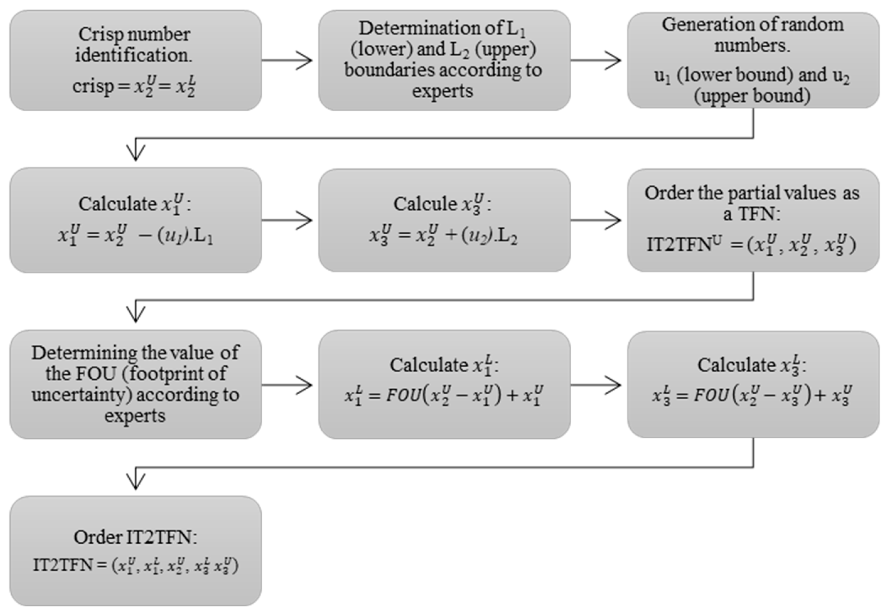
3.1. Fuzzification Method

The fuzzification method occurs in a similar way to the methods proposed by [23,24]. They used random variables to transform crisp numbers into fuzzy numbers. Uniformly distributed random variables were obtained using a random number generator herein. These variables are used to multiply lower and upper bounds (L₁ and L₂), respectively, and this process can also be used to transform crisp numbers into type-1 fuzzy numbers.

Type-1 fuzzy values should be coupled with a convenient value of FOU in order to obtain a type-2 fuzzy number (according to experts).

Crisp numbers were transformed into IT2TFN (interval type-2 triangular fuzzy numbers), where IT2TFN = (${\mathrm{x}}_1^{\mathrm{U}}$, ${\mathrm{x}}_1^{\mathrm{L}}$, ${\mathrm{x}}_2^{\mathrm{U}},{ \mathrm{x}}_3^{\mathrm{L}}$, ${\mathrm{x}}_3^{\mathrm{U}}$), as illustrated in Figure 4:

3.2. Type Reduction and Defuzzification Method

The transformation process from an IT2TFN into a crisp value is performed through a couple of steps according to Figure 5.

Firstly, type reduction occurs by transforming a type-2 into type-1 fuzzy set by means of a type-reducing method. Subsequently, a defuzzification method is applied to obtain a crisp number.

The defuzzification method for interval type-2 triangular fuzzy numbers proposed by [26] is used herein to generate a crisp value in order to facilitate the plotting of sample observations, maintain the traditional control chart format and decide whether the monitored process is in or out of statistical control.

Let $\tilde{\mathrm{A}}=(a_1^U$, $a_1^L$, $a_2^U$=$a_2^L$, $a_3^L$, $a_3^U)$ be an IT2TFN. The defuzzification method can be applied using Equation (17):

$${\mathrm{D}}_{\mathrm{TriT}}=\frac{\frac{\left(a_{\mathrm{i}3}^{\mathrm{U}}-a_{\mathrm{i}1}^{\mathrm{U}}\right)+\left(a_{\mathrm{i}2}^{\mathrm{U}}-a_{\mathrm{i}1}^{\mathrm{U}}\right)}{3}+a_{\mathrm{i}1}^{\mathrm{U}}+\mathrm{H}\left({ \tilde{\mathrm{A}}}^{\mathrm{L}}\right)\left[\frac{\left(a_{\mathrm{i}3}^{\mathrm{L}}-a_{\mathrm{i}1}^{\mathrm{L}}\right)+\left(a_{i2}^L-a_{\mathrm{i}1}^{\mathrm{L}}\right)}{3}\right]}{2}$$

(17)

In order to compare $\overline{\mathrm{X}}$ and R interval type-2 fuzzy control charts (IT2TFN) with traditional $\overline{\mathrm{X}}$ and R control charts, there must be type reduction followed by defuzzification.

As calculated values are similar to crisp values, the interval type-2 fuzzy control charts for triangular fuzzy numbers generated by these methods are similar to traditional control charts. Therefore, the presented reduction and defuzzification methods can evaluate the process as being “in control” and “out of control” in the same way as the traditional (statistical) method. The defuzzification method proposed by [26] allows finding the plotted parameters which can be defuzzied by Equations (18) and (19):

$${ \overline{\mathrm{x}} \mathrm{D}}_{\mathrm{TriT}}=\frac{\frac{\left({ \overline{\mathrm{x}}}_{\mathrm{i}3}^{\mathrm{U}}-{ \overline{\mathrm{x}}}_{\mathrm{i}1}^{\mathrm{U}}\right)+\left({ \overline{\mathrm{x}}}_{\mathrm{i}2}^{\mathrm{U}}-{ \overline{\mathrm{x}}}_{\mathrm{i}1}^{\mathrm{U}}\right)}{3}+{ \overline{\mathrm{x}}}_{\mathrm{i}1}^{\mathrm{U}}+\mathrm{H}\left({ \tilde{\mathrm{A}}}^{\mathrm{L}}\right)\left[\frac{\left({ \overline{\mathrm{x}}}_{\mathrm{i}3}^{\mathrm{L}}-{ \overline{\mathrm{x}}}_{\mathrm{i}1}^{\mathrm{L}}\right)+\left({ \overline{\mathrm{x}}}_{\mathrm{i}2}^{\mathrm{L}}-{ \overline{\mathrm{x}}}_{\mathrm{i}1}^{\mathrm{L}}\right)}{3}\right]}{2}$$

(18)

$${\mathrm{RD}}_{\mathrm{TriT}}=\frac{\frac{\left({\mathrm{R}}_{\mathrm{i}3}^{\mathrm{U}}-{\mathrm{R}}_{\mathrm{i}1}^{\mathrm{U}}\right)+\left({\mathrm{R}}_{\mathrm{i}2}^{\mathrm{U}}-{\mathrm{R}}_{\mathrm{i}1}^{\mathrm{U}}\right)}{3}+{\mathrm{R}}_{\mathrm{i}1}^{\mathrm{U}}+\mathrm{H}\left({ \tilde{\mathrm{A}}}^{\mathrm{L}}\right)\left[\frac{\left({\mathrm{R}}_{\mathrm{i}3}^{\mathrm{L}}-{\mathrm{R}}_{\mathrm{i}1}^{\mathrm{L}}\right)+\left({\mathrm{R}}_{\mathrm{i}2}^{\mathrm{L}}-{\mathrm{R}}_{\mathrm{i}1}^{\mathrm{L}}\right)}{3}\right]}{2}$$

(19)

Performing the defuzzification of control limits of IT2TFN $\overline{\mathrm{X}}$results in Equations (20)–(22):

$${\mathrm{UCL}}_{\mathrm{IT}2\mathrm{TFN}}=\frac{{\stackrel{=}{\mathrm{x}}}_1^{\mathrm{U}}+{\stackrel{=}{\mathrm{x}}}_2^{\mathrm{U}}+{\stackrel{=}{\mathrm{x}}}_3^{\mathrm{U}}+{\mathrm{A}}_2\left({ \overline{\mathrm{R}}}_1^{\mathrm{U}}+{ \overline{\mathrm{R}}}_2^{\mathrm{U}}+{ \overline{\mathrm{R}}}_3^{\mathrm{U}}\right)}{6}+ \mathrm{H}\left({ \tilde{\mathrm{A}}}^{\mathrm{L}}\right)\left[\frac{{\stackrel{=}{\mathrm{x}}}_1^{\mathrm{L}}+{\stackrel{=}{\mathrm{x}}}_2^{\mathrm{L}}+{\stackrel{=}{\mathrm{x}}}_3^{\mathrm{L}}+{\mathrm{A}}_2\left({ \overline{\mathrm{R}}}_1^{\mathrm{L}}+{ \overline{\mathrm{R}}}_2^{\mathrm{L}}+{ \overline{\mathrm{R}}}_3^{\mathrm{L}}\right)}{6}\right]$$

(20)

$${\mathrm{CL}}_{\mathrm{IT}2\mathrm{TFN}}=\frac{{\stackrel{=}{\mathrm{x}}}_1^{\mathrm{U}}+{\stackrel{=}{\mathrm{x}}}_2^{\mathrm{U}}+{\stackrel{=}{\mathrm{x}}}_3^{\mathrm{U}}}{6}+ \mathrm{H}\left({ \tilde{\mathrm{A}}}^{\mathrm{L}}\right)\left[\frac{{\stackrel{=}{\mathrm{x}}}_1^{\mathrm{L}}+{\stackrel{=}{\mathrm{x}}}_2^{\mathrm{L}}+{\stackrel{=}{\mathrm{x}}}_3^{\mathrm{L}}}{6}\right]$$

(21)

$${\mathrm{LCL}}_{\mathrm{IT}2\mathrm{TFN}}=\frac{{\stackrel{=}{\mathrm{x}}}_1^{\mathrm{U}}+{\stackrel{=}{\mathrm{x}}}_2^{\mathrm{U}}+{\stackrel{=}{\mathrm{x}}}_3^{\mathrm{U}}-{\mathrm{A}}_2\left({ \mathrm{R} ¯}_1^{\mathrm{U}}+{ \overline{\mathrm{R}}}_2^{\mathrm{U}}+{ \overline{\mathrm{R}}}_3^{\mathrm{U}}\right)}{6}+ \mathrm{H}\left({ \tilde{\mathrm{A}}}^{\mathrm{L}}\right)\left[\frac{{\stackrel{=}{\mathrm{x}}}_1^{\mathrm{L}}+{\stackrel{=}{\mathrm{x}}}_2^{\mathrm{L}}+{\stackrel{=}{\mathrm{x}}}_3^{\mathrm{L}}-{\mathrm{A}}_2\left({ \overline{\mathrm{R}}}_1^{\mathrm{L}}+{ \overline{\mathrm{R}}}_2^{\mathrm{L}}+{ \overline{\mathrm{R}}}_3^{\mathrm{L}}\right)}{6}\right]$$

(22)

Similarly, the control limits for IT2TFN R they can be calculated by Equations (23)–(25):

$${\mathrm{UCL}}_{\mathrm{IT}2\mathrm{TFN}}=\frac{D_4\left({ \overline{\mathrm{R}}}_1^{\mathrm{U}}+{ \overline{\mathrm{R}}}_2^{\mathrm{U}}+{ \overline{\mathrm{R}}}_3^{\mathrm{U}}\right)}{6}+ \mathrm{H}\left({ \tilde{\mathrm{A}}}^{\mathrm{L}}\right)\left[\frac{D_4\left({ \overline{\mathrm{R}}}_1^{\mathrm{L}}+{ \overline{\mathrm{R}}}_2^{\mathrm{L}}+{ \overline{\mathrm{R}}}_3^{\mathrm{L}}\right)}{6}\right]$$

(23)

$${\mathrm{CL}}_{\mathrm{IT}2\mathrm{TFN}}=\frac{{ \overline{\mathrm{R}}}_1^{\mathrm{U}}+{ \overline{\mathrm{R}}}_2^{\mathrm{U}}+{ \overline{\mathrm{R}}}_3^{\mathrm{U}}}{6}+ \mathrm{H}\left({ \tilde{\mathrm{A}}}^{\mathrm{L}}\right)\left[\frac{{ \overline{\mathrm{R}}}_1^{\mathrm{L}}+{ \overline{\mathrm{R}}}_2^{\mathrm{L}}+{ \overline{\mathrm{R}}}_3^{\mathrm{L}}}{6}\right]$$

(24)

$${\mathrm{LCL}}_{\mathrm{IT}2\mathrm{TFN}}=\frac{D_3\left({ \overline{\mathrm{R}}}_1^{\mathrm{U}}+{ \overline{\mathrm{R}}}_2^{\mathrm{U}}+{ \overline{\mathrm{R}}}_3^{\mathrm{U}}\right)}{6}+ \mathrm{H}\left({ \tilde{\mathrm{A}}}^{\mathrm{L}}\right)\left[\frac{D_3\left({ \overline{\mathrm{R}}}_1^{\mathrm{L}}+{ \overline{\mathrm{R}}}_2^{\mathrm{L}}+{ \overline{\mathrm{R}}}_3^{\mathrm{L}}\right)}{6}\right]$$

(25)

Figure 6 and Figure 7 graphically illustrate the construction of the IT2TFN $\overline{\mathrm{X}}$-R control charts after defuzzification of the control limits and their sample observations.

The proposed model can be used in real processes whose parameters are unknown. However, for comparison purposes with traditional control charts, it is possible that its performance can be measured using known parameters.

4. Control Chart Performance Measures

In situations where processes are stabilized, i.e., free of special causes, ARL₀ is defined as the main performance measure. The ARL₀ reveals the number of samples required until there is a false alarm. This implies that a control chart indicates when a sample is out of control while it is supposedly in control [27]. According to [20], ARL₀ is the inverse of a type I error (α) as in Equation (26):

$${\mathrm{ARL}}_0=\frac{1}{\mathsf{\alpha }}$$

(26)

Another important measure concerning the performance analysis of control charts is the standard deviation of the run length (SDRL). For a better performance analysis of control charts, [28,29] state that it is important to use a performance measure associated with dispersion coupled with ARL, since ARL presents high variability. The value of SDRL₀, i.e., the expected value for a process free of special causes, can be calculated as in Equation (27):

$${\mathrm{SDRL}}_0=\frac{\sqrt{1-\mathsf{\alpha }}}{\mathsf{\alpha }}$$

(27)

From simulated RL values, it is possible to perform other statistical analyses, such as RL percentiles. Proposed by [30], RL percentiles are used to complement the ARL and SDRL analysis, since it is capable of demonstrating variation in false alarms given by control charts under study.

According to [31], an exclusive use of ARL as a performance measure may not provide a complete picture of chart performance, since both in-control and out-of-control distributions are largely skewed. The RL percentile is a robust measure of control chart performance. The 100th percentile (0 < q < 1) can be given by Equation (28):

$$1-{\beta }^m=\frac{\mathrm{q}}{100}$$

(28)

In order to compare the proposed control charts to traditional control charts, the control factor (k) of each chart must be initially adjusted individually so that when the process is under control, the two charts reach approximate values of ARL₀. Once ARL₀ values are very close, the difference in δ standard deviations of the process mean and the displacement of λ in the process range are simulated so as to compare ARL values found through a traditional control chart with those of the proposed fuzzy control chart. The one with the lowest ARL value is the most efficient for a given situation. Therefore, the most efficient graphs should reach high ARL₀ values, i.e., few false alarms and low ARL values, so as to quickly detect variations in the process mean and range [32].

Thus, according to [33,34], control charts mainly aim to monitor any random cause changing the value of the process mean in control µ₀ to µ₁ = µ₀ ± δ${\mathsf{\sigma }}_{ \overline{\mathrm{x}}}$ and/or those increasing the standard deviation in control σ₀ to σ₁ = λσ₀, where λ is the magnitude of variability increase.

The fuzzy sets used in control charts by [8] allowed performing a fuzzification method using random variables, and the performance of type-1 fuzzy $\overline{\mathrm{X}}$-R control charts was measured using the average run length (ARL) and the extra quadratic loss (EQL).

On the other hand, [9] evaluated the performance of exponentially weighted moving average (EWMA) control charts using ARLs for traditional and fuzzy control charts. Considering a process whose mean is 0 and standard deviation equals 1, triangular fuzzy numbers are subsequently found through a fuzzification method.

In this work, the ARL, SDRL and RL percentile values are simulated as performance measures. The simulation algorithm, considering known parameters, can be seen in Figure 8.

In order to obtain the ARL, SDRL and RL percentile measurements, the $\overline{\mathrm{X}}$-R control charts were considered together. According to [20], the $\overline{\mathrm{X}}$ and R control charts should be applied together in such a way that both the mean and variability of processes can be monitored. Once a sample is shown to be out of control, either by means of the $\overline{\mathrm{X}}$ or R control chart, the process must be stopped so that corrective action can be taken.

5. Results and Discussion

To simulate ARL, SDRL and RL percentiles of IT2TFN $\overline{\mathrm{X}}$ and R control charts, sample size n = 5, process mean 0.0 and standard deviation 1.0 were selected. L₁ = L₂ = 0.05 and FOU = 0.30 were used in the fuzzification process according to experts, as they provide a fast response while at the same time reducing overshoots according to [18].

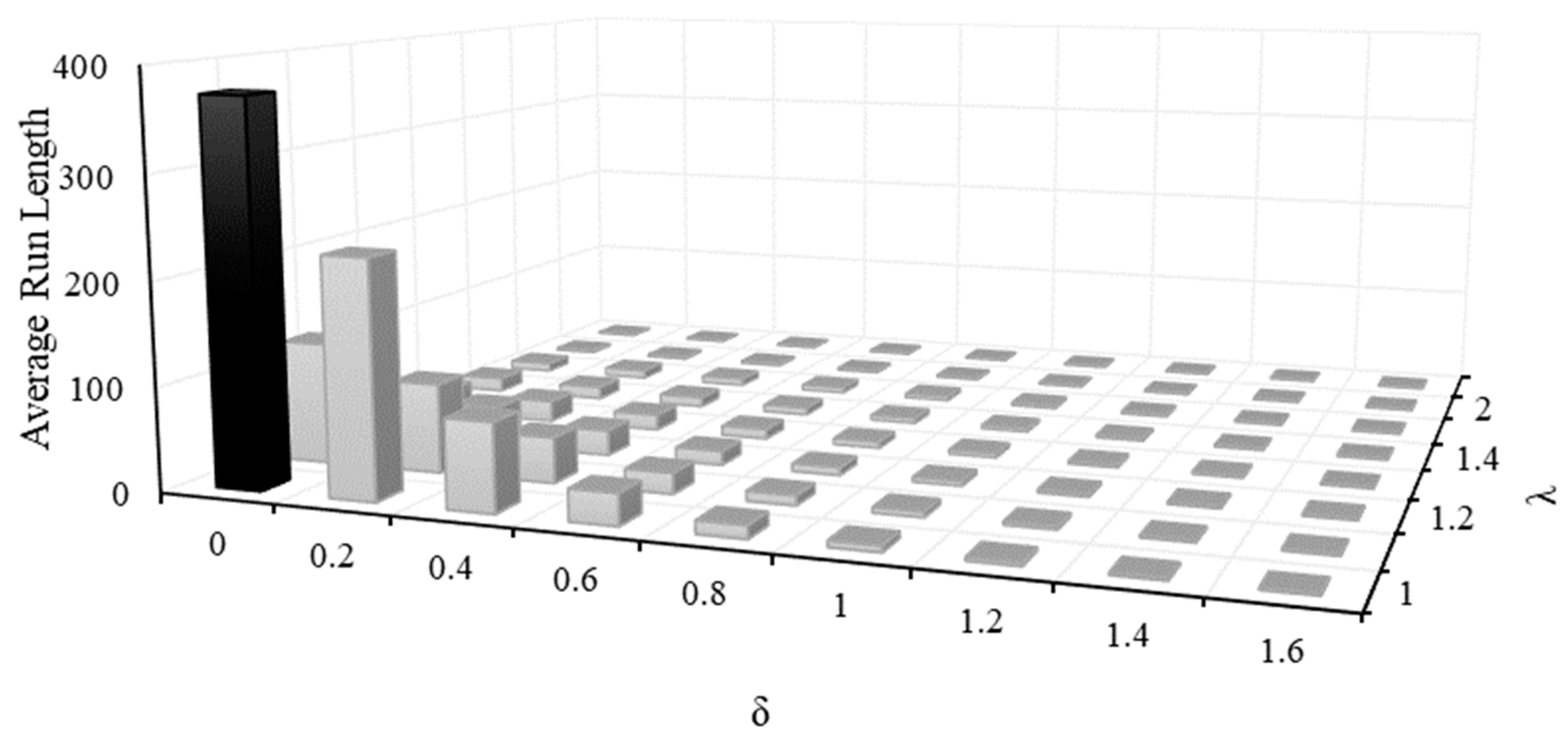
5.1. Average Run Length (ARL) and Standard Deviation Run Length (SDRL) for $\overline{X}$-R Control Charts

The values of δ range from 0 to 1.6 with successive increments of 0.2, and λ ranges from 1 to 2.5. According [34], 10,000 iterations were performed in the simulation in order to reach a more accurate result.

Table 2. Theoretical values of ARL and SDRL found for traditional $\overline{\mathrm{X}}$ and R control charts.

Traditional $\overline{X}$-R Control Chart ARL
λ	δ (Shift)
#	0.0	0.2	0.4	0.6	0.8	1.0	1.2	1.4	1.6
1.0	370.5	228.0	84.9	30.8	12.6	6.0	3.3	2.1	1.5
1.1	119.2	88.2	44.1	20.1	9.7	5.2	3.1	2.1	1.6
1.2	48.8	40.3	25.0	13.8	7.7	4.5	2.9	2.1	1.6
1.3	24.2	21.3	15.3	9.8	6.2	4.0	2.8	2.0	1.6
1.4	13.9	12.8	10.1	7.2	5.0	3.5	2.6	2.0	1.6
1.5	8.9	8.4	7.1	5.5	4.2	3.1	2.4	1.9	1.6
2.0	2.6	2.5	2.4	2.3	2.1	1.9	1.7	1.5	1.4
2.5	1.6	1.6	1.5	1.5	1.5	1.4	1.4	1.3	1.2
	Traditional $\overline{X}$-R Control Chart SDRL
λ	δ (Shift)
#	0.0	0.2	0.4	0.6	0.8	1.0	1.2	1.4	1.6
1.0	370.0	227.5	84.4	30.2	12.1	5.5	2.8	1.5	0.9
1.1	118.7	87.7	43.6	19.6	9.2	4.7	2.6	1.5	1.0
1.2	48.3	39.8	24.4	13.3	7.1	4.0	2.4	1.5	1.0
1.3	23.7	20.8	14.8	9.3	5.6	3.5	2.2	1.4	1.0
1.4	13.4	12.2	9.5	6.7	4.5	3.0	2.0	1.4	1.0
1.5	8.4	7.9	6.5	5.0	3.6	2.6	1.8	1.3	1.0
2.0	2.0	2.0	1.8	1.7	1.5	1.3	1.1	0.9	0.8
2.5	0.9	0.9	0.9	0.9	0.8	0.8	0.7	0.6	0.6

presents the theoretical values of ARL and SDRL performance measures found for traditional control charts. It is observed that the SDRL value is very close to that of ARL, which explains the high variability of ARL as a performance measure.

Although not starting from an ARL = 370.50, IT2TFN control charts showed an average reduction by 0.31% and 0.33% in ARL and SDRL values, respectively, when compared to values found using traditional control charts.

ARL values whose δ = 0.8 showed 1.37% lower values (on average) with respect to the same δ value simulated in traditional control charts. Regarding λ, ARL values were found when λ = 1.40 and showed 0.76% lower ARL considering the same λ value simulated in traditional control charts, as shown in

Table 3. Simulated values of ARL and SDRL found for IT2TFN $\overline{\mathrm{X}}$ and R control charts.

IT2TFN $\overline{X}$-R Control Chart ARL
λ	δ (Shift)
#	0.0	0.2	0.4	0.6	0.8	1.0	1.2	1.4	1.6
1.0	372.45	228.54	85.32	30.43	12.55	5.93	3.35	2.11	1.56
1.1	118.56	87.10	44.23	20.32	9.56	5.17	3.11	2.10	1.59
1.2	48.54	39.54	24.89	13.77	7.67	4.54	2.95	2.08	1.58
1.3	24.10	21.09	15.45	9.71	6.14	4.03	2.76	2.00	1.60
1.4	13.91	12.61	9.77	7.27	4.99	3.50	2.56	1.97	1.60
1.5	8.70	8.33	7.06	5.52	4.10	3.08	2.41	1.92	1.59
2.0	2.56	2.50	2.42	2.29	2.05	1.87	1.70	1.54	1.42
2.5	1.57	1.55	1.54	1.50	1.45	1.40	1.36	1.29	1.26
IT2TFN $\overline{X}$-R Control Chart SDRL
λ	δ (Shift)
#	0.0	0.2	0.4	0.6	0.8	1.0	1.2	1.4	1.6
1.0	371.141	226.537	84.860	29.844	12.081	5.298	2.807	1.515	0.942
1.1	119.090	85.087	43.340	19.960	9.167	4.605	2.551	1.528	0.972
1.2	47.318	39.034	24.456	13.138	7.122	3.997	2.400	1.491	0.964
1.3	23.366	20.641	14.992	9.222	5.628	3.549	2.208	1.407	0.968
1.4	13.220	12.266	9.299	6.628	4.510	3.012	1.981	1.397	0.987
1.5	8.180	7.808	6.506	4.924	3.534	2.526	1.880	1.346	0.964
2.0	2.042	1.975	1.879	1.735	1.482	1.296	1.094	0.910	0.774
2.5	0.938	0.938	0.918	0.869	0.827	0.742	0.697	0.614	0.576

.

For SDRL, there is an average reduction by 2.13% considering δ = 1.6, but 0.98% in SRDL when λ = 1.2 in comparison with traditional control charts. Such reductions in ARL and SDRL demonstrate that IT2TFN $\overline{\mathrm{X}}$ and R control charts are capable of detecting out-of-control points more accurately than traditional control charts. Thus, the presently proposed model has superior performance.

A rapid response is observed when the purpose of process monitoring is to detect defects from a quality characteristic, which is a variable able to be obtained by a measurement system in the case under study.

Regarding the behavior of RLs, [29] reports that ARL and SDRL values at every δ and λ value should be close, since ARL and SDRL performance metrics are in accordance with a geometric distribution. Figure 9 and Figure 10 illustrate the values of ARL and SDRL as a function of δ and λ, respectively. It is worth mentioning that they are quite similar in terms of shape and numerical scale.

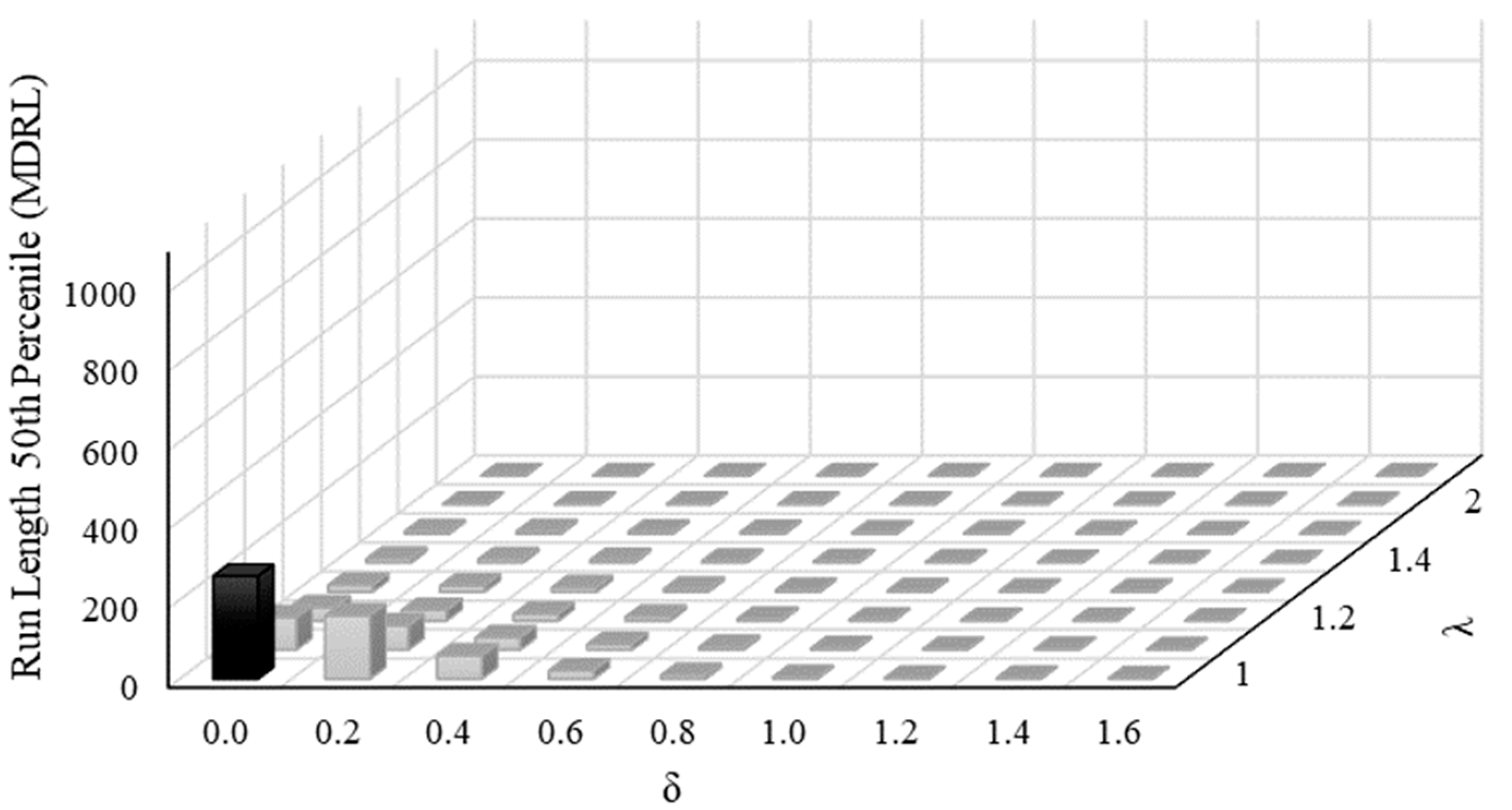
5.2. Run Length Percentile Analysis for $\overline{X}$-R Control Charts

Table 4. Theoretical values of RL Percentiles (5th, 25th, 50th, 75th and 95th) found for traditional $\overline{\mathrm{X}}$ and R control charts. The percentiles are divided into sub-tables.

5th	λ	δ (Shift)									25th	λ	δ (Shift)
	#	0.0	0.2	0.4	0.6	0.8	1.0	1.2	1.4	1.6		#	0.0	0.2	0.4	0.6	0.8	1.0	1.2	1.4	1.6
	1.0	19	12	5	2	1	1	1	1	1		1.0	107	66	25	9	4	2	1	1	1
	1.1	7	5	3	2	1	1	1	1	1		1.1	35	26	13	6	3	2	1	1	1
	1.2	3	3	2	1	1	1	1	1	1		1.2	14	12	8	4	3	2	1	1	1
	1.3	2	2	1	1	1	1	1	1	1		1.3	7	6	5	3	2	2	1	1	1
	1.4	1	1	1	1	1	1	1	1	1		1.4	4	4	3	2	2	1	1	1	1
	1.5	1	1	1	1	1	1	1	1	1		1.5	3	3	2	2	2	1	1	1	1
	2.0	1	1	1	1	1	1	1	1	1		2.0	1	1	1	1	1	1	1	1	1
	2.5	1	1	1	1	1	1	1	1	1		2.5	1	1	1	1	1	1	1	1	1
50th (MDRL)	λ	δ (Shift)
	#	0.0	0.2	0.4	0.6	0.8	1.0	1.2	1.4	1.6
	1.0	257	158	59	21	9	4	2	2	1
	1.1	83	61	31	14	7	4	2	2	1
	1.2	34	28	17	10	5	3	2	2	1
	1.3	17	15	11	7	4	3	2	2	1
	1.4	10	9	7	5	4	3	2	1	1
	1.5	6	6	5	4	3	2	2	1	1
	2.0	2	2	2	2	2	1	1	1	1
	2.5	1	1	1	1	1	1	1	1	1
75th	λ	δ (Shift)									95th	λ	δ (Shift)
	#	0.0	0.2	0.4	0.6	0.8	1.0	1.2	1.4	1.6		#	0.0	0.2	0.4	0.6	0.8	1.0	1.2	1.4	1.6
	1.0	513	316	117	42	17	8	4	3	2		1.0	1109	682	253	91	37	17	9	5	3
	1.1	165	122	61	28	13	7	4	3	2		1.1	356	263	131	59	28	14	8	5	3
	1.2	67	56	34	19	10	6	4	3	2		1.2	145	120	74	40	22	13	8	5	4
	1.3	33	29	21	13	8	5	4	3	2		1.3	72	63	45	28	17	11	7	5	4
	1.4	19	17	14	10	7	5	3	2	2		1.4	41	37	29	21	14	10	7	5	4
	1.5	12	11	10	7	6	4	3	2	2		1.5	26	24	20	15	11	8	6	5	4
	2.0	3	3	3	3	3	2	2	2	2		2.0	7	6	6	6	5	4	4	3	3
	2.5	2	2	2	2	2	2	2	1	1		2.5	3	3	3	3	3	3	3	3	2

presents the theoretical values of RL percentiles found for the traditional control chart. It should be noted that the 50th percentile for the in-control situation, i.e., considering δ = 0.0 and λ = 1.0, indicates that there is a false alarm within the first 257 samples, at least half the time. The initial 5th percentile for δ = 0.0 and λ = 1.0 allowed evidencing early false alarms. There is a 5% probability that there will be a first false alarm in less than 19 measurements.

Table 5. Simulated values of RL Percentiles (5th, 25th, 50th, 75th and 95th) for IT2TFN $\overline{\mathrm{X}}$ and R control charts. The percentiles are divided into sub-tables.

5th	λ	δ (Shift)									25th	λ	δ (Shift)
	#	0.0	0.2	0.4	0.6	0.8	1.0	1.2	1.4	1.6		#	0.0	0.2	0.4	0.6	0.8	1.0	1.2	1.4	1.6
	1.0	20	13	5	2	1	1	1	1	1		1.0	107	67	25	9	4	2	1	1	1
	1.1	7	5	3	2	1	1	1	1	1		1.1	34	26	13	6	3	2	1	1	1
	1.2	3	2	2	1	1	1	1	1	1		1.2	15	12	8	4	3	2	1	1	1
	1.3	2	2	1	1	1	1	1	1	1		1.3	7	6	5	3	2	2	1	1	1
	1.4	1	1	1	1	1	1	1	1	1		1.4	4	4	3	3	2	1	1	1	1
	1.5	1	1	1	1	1	1	1	1	1		1.5	3	3	2	2	2	1	1	1	1
	2.0	1	1	1	1	1	1	1	1	1		2.0	1	1	1	1	1	1	1	1	1
	2.5	1	1	1	1	1	1	1	1	1		2.5	1	1	1	1	1	1	1	1	1
50th (MDRL)	λ	δ (Shift)
	#	0.0	0.2	0.4	0.6	0.8	1.0	1.2	1.4	1.6
	1.0	260	160	59	21	9	4	2	2	1
	1.1	82	61	31	14	7	4	2	2	1
	1.2	34	27	17	10	5	3	2	2	1
	1.3	17	15	11	7	4	3	2	2	1
	1.4	10	9	7	5	4	3	2	1	1
	1.5	6	6	5	4	3	2	2	1	1
	2.0	2	2	2	2	2	1	1	1	1
	2.5	1	1	1	1	1	1	1	1	1
75th	λ	δ (Shift)									95th	λ	δ (Shift)
	#	0.0	0.2	0.4	0.6	0.8	1.0	1.2	1.4	1.6		#	0.0	0.2	0.4	0.6	0.8	1.0	1.2	1.4	1.6
	1.0	517	317	118	42	17	8	4	3	2		1.0	1098	682	258	91	37	17	9	5	3
	1.1	164	122	61	28	13	7	4	3	2		1.1	358	257	130	60	28	14	8	5	4
	1.2	67	55	34	19	10	6	4	3	2		1.2	142	118	75	41	22	12.1	8	5	4
	1.3	33	29	21	13	8	5	4	3	2		1.3	71	62	46	28	17	11	7	5	4
	1.4	19	17	13	10	7	5	3	2	2		1.4	41	37	29	20	14	9	7	5	4
	1.5	12	11	10	8	5	4	3	2	2		1.5	25	24	20	15	11	8	6	5	3
	2.0	3	3	3	3	3	2	2	2	2		2.0	7	6	6	6	5	4	4	3	3
	2.5	2	2	2	2	2	2	2	1	1		2.5	3	3	3	3	3	3	3	3	2

presents the simulated values of RL percentiles found for IT2TFN control charts. It should be noted that MDRL (50th percentile) considering a scenario which is in control, i.e., δ = 0.0 and λ = 1.0, indicates that there is a false alarm within the first 260 samples at least half the time. The initial 5th percentile for δ = 0.0 and λ = 1.0 allowed evidencing early false alarm. There is a 5% probability that there will be a first false alarm in less than 20 measurements.

In contrast, it was observed that RL percentile values for IT2TFN $\overline{\mathrm{X}}$ and R control charts are quite similar to those found through traditional control charts. However, on an overall average, small reductions in RL percentile values shown by the proposed charts demonstrate a slightly greater propensity for false alarms.

For situations in which the process is in control, the proposed charts generally take longer to reveal false alarms if compared to traditional control charts. Figure 11 illustrates the 50th percentile, i.e., the MDRL.

Thus, IT2TFN $\overline{\mathrm{X}}$ and R control charts offer several overwhelming advantages over traditional $\overline{\mathrm{X}}$ and R control charts.

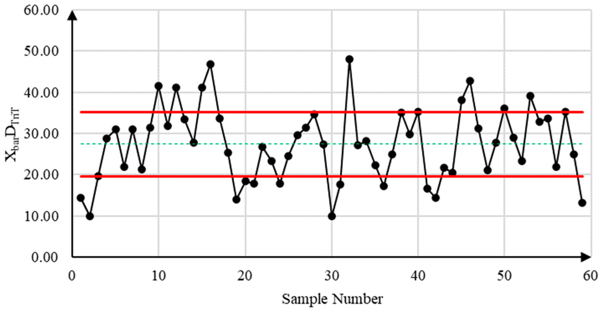
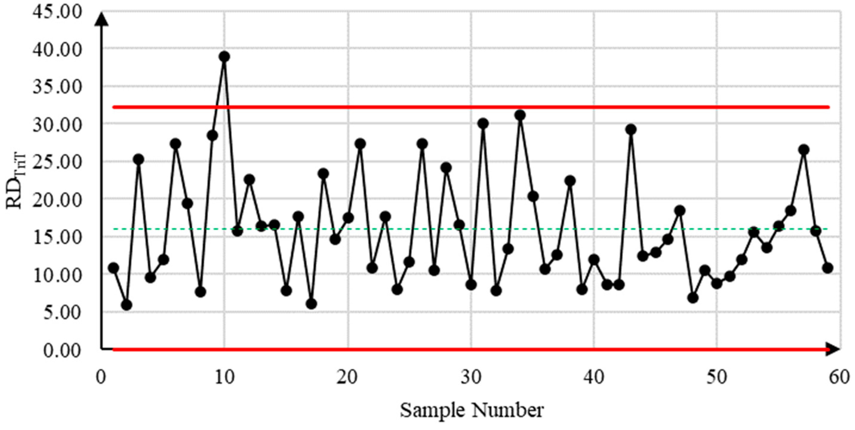
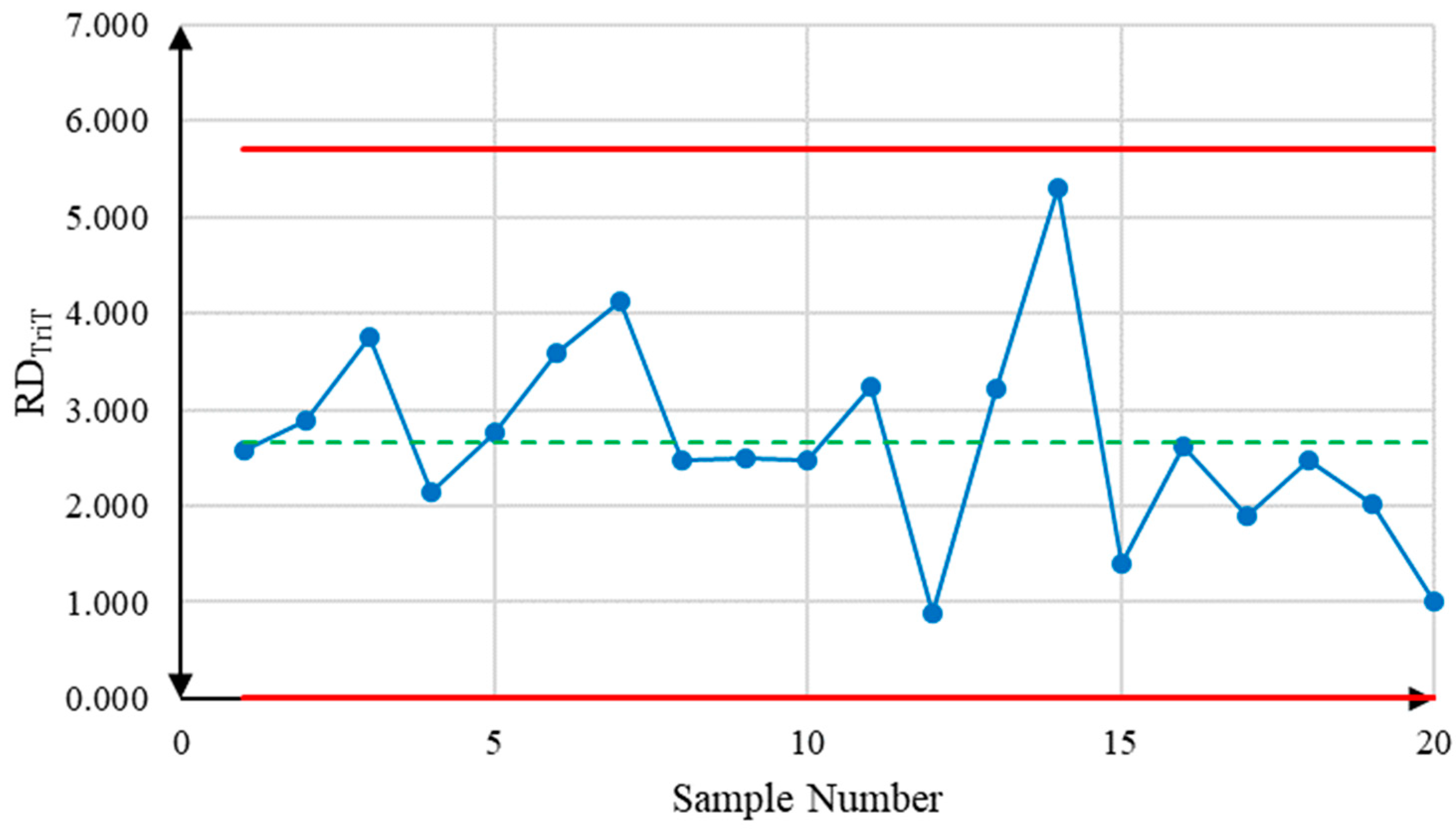
5.3. Illustrative Example

After the performance analysis, in order to understand how the proposed model can be implemented in real processes, we use an illustrative example. Considering a process whose mean is 0 and standard deviation is 1, 20 samples are randomly generated whose sample subgroups have a size of 5. Using the control limit equations for the traditional $\overline{X}$ and R control charts, as can be seen in [18], we obtain: LCL = −1.477 and UCL = 1.480 for $\overline{\mathrm{X}}$; and LCL = 0 and UCL = 5.417 for R.

Table 6. Example for traditional $\overline{X}$ and R control charts (normal distribution, µ = 0.0 and σ = 1.0.

Sample Number	Measures (Crisp Values)					Variables		Decision
	x1	x2	x3	x4	x5	$\overline{\mathbf{x}}$	R
1	−0.547	−0.551	1.866	−0.418	−0.706	−0.071	2.572	In control
2	−0.382	0.075	−1.504	1.395	−0.152	−0.114	2.899	In control
3	0.694	−0.444	−1.559	1.975	−1.800	−0.227	3.776	In control
4	0.050	−0.520	−1.425	−0.194	0.721	−0.273	2.146	In control
5	1.368	0.014	−0.207	0.518	−1.400	0.059	2.769	In control
6	1.615	0.706	−0.783	−0.620	−1.980	−0.212	3.595	In control
7	−2.426	1.077	0.569	1.686	−0.859	0.009	4.112	In control
8	1.824	0.195	−0.659	−0.415	−0.581	0.073	2.483	In control
9	0.646	−0.241	−1.400	−1.045	1.090	−0.190	2.490	In control
10	1.101	−0.685	1.772	0.372	−0.337	0.445	2.457	In control
11	0.259	−2.005	1.247	1.204	0.223	0.186	3.252	In control
12	−0.104	−0.320	−0.968	−0.484	−0.337	−0.443	0.864	In control
13	−2.235	−0.614	0.234	0.991	−0.096	−0.344	3.226	In control
14	2.216	−0.527	−3.062	0.176	0.155	−0.208	5.278	In control
15	0.960	0.729	0.772	0.304	1.699	0.893	1.395	In control
16	−0.199	2.435	0.528	0.906	0.547	0.843	2.634	In control
17	1.416	−0.461	−0.244	0.202	−0.058	0.171	1.878	In control
18	1.633	−0.748	−0.642	−0.832	0.872	0.056	2.465	In control
19	0.064	0.758	−0.515	1.516	0.671	0.499	2.031	In control
20	0.292	−0.551	−0.362	0.309	0.449	0.027	1.000	In control

shows the situation described, together with the $\overline{\mathrm{X}}$ and R parameters.

As can be seen in Table 6, all the samples are in control, which indicates that the process is stable. Applying the proposed fuzzification method, considering the lower and upper bounds L₁ = L₂ = 0.05, according to experts, FOU equals 0.30 and considering H(${\tilde{A}}^U$) = H(${\tilde{A}}^L$) = 1. The crisp numbers obtained for the traditional $\overline{\mathrm{X}}$ and R control charts was used with $x_2^U$ = $x_2^L$ (center value) and is used as a basis for obtaining the other interval type−2 fuzzy values. After the fuzzification process, as can be seen in Figure 4, we calculate the sample means ${ \overline{\mathrm{x}}}_{\mathrm{IT}2\mathrm{TFN}}=\left({ \overline{\mathrm{x}}}_{\mathrm{i}1}^{\mathrm{U}},{ \overline{\mathrm{x}}}_{\mathrm{i}1}^{\mathrm{L}},{ \overline{\mathrm{x}}}_{\mathrm{i}2}^{\mathrm{U}},{ \overline{\mathrm{x}}}_{\mathrm{i}3}^{\mathrm{L}},{ \overline{\mathrm{x}}}_{\mathrm{i}3}^{\mathrm{U}}\right)$ and sample ranges $R_{IT2TFN}=\left(R_{i1}^U,R_{i1}^L, R_{i2}^U, R_{i3}^L, R_{i3}^U\right)$, where i is the number of the measurements obtained (

Table 7. Fuzzified numbers of illustrative example on an interval type−2 triangular fuzzy number approach.

Sample Number	x1					x2					x3					x4					x5
	${\mathbf{x}}_{11}^{\mathbf{U}}$	${\mathbf{x}}_{11}^{\mathbf{L}}$	${\mathbf{x}}_{12}^{\mathbf{U}}$	${\mathbf{x}}_{13}^{\mathbf{L}}$	${\mathbf{x}}_{13}^{\mathbf{U}}$	${\mathbf{x}}_{21}^{\mathbf{U}}$	${\mathbf{x}}_{21}^{\mathbf{L}}$	${\mathbf{x}}_{22}^{\mathbf{U}}$	${\mathbf{x}}_{23}^{\mathbf{L}}$	${\mathbf{x}}_{23}^{\mathbf{U}}$	${\mathbf{x}}_{31}^{\mathbf{U}}$	${\mathbf{x}}_{31}^{\mathbf{L}}$	${\mathbf{x}}_{32}^{\mathbf{U}}$	${\mathbf{x}}_{33}^{\mathbf{L}}$	${\mathbf{x}}_{33}^{\mathbf{U}}$	${\mathbf{x}}_{41}^{\mathbf{U}}$	${\mathbf{x}}_{41}^{\mathbf{L}}$	${\mathbf{x}}_{42}^{\mathbf{U}}$	${\mathbf{x}}_{43}^{\mathbf{L}}$	${\mathbf{x}}_{43}^{\mathbf{U}}$	${\mathbf{x}}_{51}^{\mathbf{U}}$	${\mathbf{x}}_{51}^{\mathbf{L}}$	${\mathbf{x}}_{52}^{\mathbf{U}}$	${\mathbf{x}}_{53}^{\mathbf{L}}$	${\mathbf{x}}_{53}^{\mathbf{U}}$
1	−0.587	−0.575	−0.547	−0.526	−0.517	−0.566	−0.561	−0.551	−0.535	−0.528	1.838	1.846	1.866	1.890	1.900	−0.461	−0.448	−0.418	−0.391	−0.380	−0.736	−0.727	−0.706	−0.696	−0.692
2	−0.418	−0.407	−0.382	−0.349	−0.335	0.028	0.042	0.075	0.078	0.080	−1.534	−1.525	−1.504	−1.485	−1.477	1.346	1.361	1.395	1.406	1.411	−0.177	−0.170	−0.152	−0.144	−0.140
3	0.687	0.689	0.694	0.698	0.700	−0.466	−0.459	−0.444	−0.410	−0.395	−1.608	−1.593	−1.559	−1.556	−1.555	1.932	1.945	1.975	1.996	2.004	−1.817	−1.812	−1.800	−1.770	−1.758
4	0.008	0.021	0.050	0.079	0.091	−0.538	−0.532	−0.520	−0.488	−0.474	−1.428	−1.427	−1.425	−1.402	−1.392	−0.209	−0.204	−0.194	−0.167	−0.155	0.690	0.700	0.721	0.743	0.752
5	1.341	1.349	1.368	1.372	1.374	−0.025	−0.013	0.014	0.041	0.053	−0.241	−0.231	−0.207	−0.205	−0.204	0.482	0.493	0.518	0.537	0.545	−1.406	−1.404	−1.400	−1.377	−1.367
6	1.607	1.609	1.615	1.624	1.628	0.661	0.674	0.706	0.726	0.735	−0.822	−0.810	−0.783	−0.749	−0.734	−0.623	−0.622	−0.620	−0.599	−0.589	−1.989	−1.986	−1.980	−1.967	−1.961
7	−2.475	−2.460	−2.426	−2.409	−2.401	1.067	1.070	1.077	1.112	1.127	0.537	0.547	0.569	0.576	0.579	1.664	1.671	1.686	1.701	1.708	−0.866	−0.864	−0.859	−0.849	−0.845
8	1.810	1.815	1.824	1.840	1.847	0.165	0.174	0.195	0.218	0.229	−0.673	−0.669	−0.659	−0.631	−0.618	−0.441	−0.433	−0.415	−0.412	−0.410	−0.611	−0.602	−0.581	−0.567	−0.561
9	0.626	0.632	0.646	0.646	0.647	−0.249	−0.247	−0.241	−0.232	−0.228	−1.409	−1.406	−1.400	−1.395	−1.393	−1.046	−1.046	−1.045	−1.024	−1.015	1.087	1.088	1.090	1.113	1.122
10	1.100	1.100	1.101	1.120	1.128	−0.724	−0.712	−0.685	−0.681	−0.679	1.737	1.748	1.772	1.796	1.806	0.323	0.338	0.372	0.381	0.385	−0.350	−0.346	−0.337	−0.321	−0.315
11	0.236	0.243	0.259	0.270	0.275	−2.014	−2.011	−2.005	−1.982	−1.973	1.206	1.218	1.247	1.254	1.257	1.201	1.202	1.204	1.222	1.230	0.220	0.221	0.223	0.252	0.265
12	−0.111	−0.109	−0.104	−0.076	−0.064	−0.341	−0.335	−0.320	−0.308	−0.303	−1.018	−1.003	−0.968	−0.940	−0.927	−0.502	−0.497	−0.484	−0.468	−0.461	−0.354	−0.349	−0.337	−0.312	−0.302
13	−2.281	−2.267	−2.235	−2.203	−2.189	−0.662	−0.648	−0.614	−0.609	−0.607	0.197	0.208	0.234	0.265	0.279	0.973	0.979	0.991	1.006	1.012	−0.112	−0.107	−0.096	−0.088	−0.085
14	2.214	2.215	2.216	2.246	2.259	−0.569	−0.556	−0.527	−0.508	−0.501	−3.088	−3.080	−3.062	−3.061	−3.061	0.140	0.150	0.176	0.206	0.218	0.150	0.151	0.155	0.184	0.197
15	0.950	0.953	0.960	0.971	0.975	0.680	0.695	0.729	0.744	0.750	0.763	0.766	0.772	0.797	0.808	0.263	0.276	0.304	0.309	0.312	1.656	1.669	1.699	1.703	1.705
16	−0.244	−0.230	−0.199	−0.176	−0.166	2.389	2.403	2.435	2.444	2.447	0.499	0.508	0.528	0.538	0.543	0.878	0.886	0.906	0.913	0.917	0.524	0.531	0.547	0.576	0.589
17	1.401	1.405	1.416	1.450	1.465	−0.494	−0.484	−0.461	−0.439	−0.430	−0.286	−0.274	−0.244	−0.242	−0.242	0.160	0.172	0.202	0.217	0.223	−0.101	−0.088	−0.058	−0.032	−0.021
18	1.632	1.632	1.633	1.633	1.634	−0.780	−0.771	−0.748	−0.714	−0.699	−0.659	−0.654	−0.642	−0.622	−0.613	−0.844	−0.840	−0.832	−0.827	−0.825	0.855	0.860	0.872	0.896	0.906
19	0.015	0.030	0.064	0.098	0.113	0.740	0.745	0.758	0.774	0.781	−0.521	−0.519	−0.515	−0.490	−0.480	1.491	1.498	1.516	1.546	1.559	0.650	0.656	0.671	0.703	0.717
20	0.269	0.276	0.292	0.295	0.297	−0.575	−0.568	−0.551	−0.549	−0.548	−0.412	−0.397	−0.362	−0.352	−0.347	0.278	0.288	0.309	0.343	0.358	0.420	0.429	0.449	0.457	0.461

).

In order to compare IT2TFN $\overline{\mathrm{X}}$ and R control charts with the traditional control charts, it is important that the fuzzified values of ${ \overline{\mathrm{X}}}_{\mathrm{IT}2\mathrm{TFN}}$ and ${\mathrm{R}}_{\mathrm{IT}2\mathrm{TFN}}$ are defuzzied, according to Equations (18) and (19). The defuzzied$\overline{\mathrm{X}}$D_TriT and RD_TriT values are plotted in the control charts. The fuzzified and defuzzied data can be seen in

Table 8. Fuzzified and defuzzied values of $\overline{\mathrm{X}}$ and R from an illustrative example on an interval type−2 triangular fuzzy number approach.

Sample Number	$\mathbf{Mean} {\overline{\mathbf{X}}}_{\mathbf{I}\mathbf{T}2\mathbf{T}\mathbf{F}\mathbf{N}}$					$\mathbf{Range} {\mathbf{R}}_{\mathbf{I}\mathbf{T}2\mathbf{T}\mathbf{F}\mathbf{N}}$					Defuzzified
	${\overline{\mathbf{X}}}_1^{\mathbf{U}}$	${\overline{\mathbf{X}}}_1^{\mathbf{L}}$	${\overline{\mathbf{X}}}_2^{\mathbf{U}}$	${\overline{\mathbf{X}}}_3^{\mathbf{L}}$	${\overline{\mathbf{X}}}_3^{\mathbf{U}}$	${\mathbf{R}}_1^{\mathbf{U}}$	${\mathbf{R}}_1^{\mathbf{L}}$	${\mathbf{R}}_2^{\mathbf{U}}$	${\mathbf{R}}_3^{\mathbf{L}}$	${\mathbf{R}}_3^{\mathbf{U}}$	$\overline{\mathbf{X}}$DTriT	RDTriT
1	−0.102	−0.093	−0.071	−0.052	−0.043	2.529	2.542	2.572	2.617	2.636	−0.072	2.578
2	−0.151	−0.140	−0.114	−0.099	−0.092	2.822	2.846	2.899	2.931	2.945	−0.118	2.890
3	−0.254	−0.246	−0.227	−0.209	−0.201	3.690	3.715	3.776	3.808	3.821	−0.227	3.764
4	−0.295	−0.289	−0.273	−0.247	−0.235	2.082	2.101	2.146	2.170	2.180	−0.269	2.138
5	0.030	0.039	0.059	0.074	0.080	2.708	2.726	2.769	2.777	2.780	0.057	2.755
6	−0.233	−0.227	−0.212	−0.193	−0.184	3.568	3.576	3.595	3.610	3.617	−0.210	3.594
7	−0.014	−0.007	0.009	0.026	0.033	4.065	4.079	4.112	4.161	4.183	0.009	4.119
8	0.050	0.057	0.073	0.090	0.097	2.429	2.445	2.483	2.510	2.521	0.073	2.478
9	−0.198	−0.196	−0.190	−0.179	−0.174	2.480	2.483	2.490	2.519	2.531	−0.188	2.499
10	0.417	0.426	0.445	0.459	0.465	2.417	2.429	2.457	2.508	2.530	0.443	2.466
11	0.170	0.175	0.186	0.203	0.211	3.179	3.201	3.252	3.265	3.271	0.188	3.236
12	−0.465	−0.459	−0.443	−0.421	−0.411	0.816	0.830	0.864	0.927	0.954	−0.440	0.876
13	−0.377	−0.367	−0.344	−0.326	−0.318	3.162	3.181	3.226	3.273	3.293	−0.346	3.227
14	−0.231	−0.224	−0.208	−0.187	−0.177	5.275	5.276	5.278	5.327	5.347	−0.206	5.297
15	0.863	0.872	0.893	0.905	0.910	1.344	1.360	1.395	1.428	1.442	0.889	1.394
16	0.809	0.820	0.843	0.859	0.866	2.555	2.579	2.634	2.674	2.691	0.840	2.628
17	0.136	0.146	0.171	0.191	0.199	1.831	1.845	1.878	1.934	1.959	0.169	1.887
18	0.041	0.045	0.056	0.073	0.081	2.457	2.459	2.465	2.474	2.477	0.059	2.466
19	0.475	0.482	0.499	0.526	0.538	1.970	1.988	2.031	2.065	2.080	0.503	2.028
20	−0.004	0.006	0.027	0.039	0.044	0.968	0.978	1.000	1.025	1.035	0.023	1.001

.

Since the values of $\stackrel{=}{\mathrm{X}}$ = (0.033, 0.041, 0.059, 0.077, 0.084) and$\overline{\mathrm{R}}$ = (2.617, 2.632, 2.666, 2.700, 2.715), and considering the variables A₂ = 0.577, D₃ = 0.000 and D₄ = 2.114, it is possible to calculate the defuzzied IT2TFN$\overline{\mathrm{X}}$ and R control limits.

Based on the data presented in Table 8, one can calculate the control limits for the IT2TFN$\overline{\mathrm{X}}$ control chart using Equations (20)–(22). Similarly, to calculate the control limits of the IT2TFN R control chart, we use Equations (23)–(25). The IT2TFN$\overline{\mathrm{X}}$ and IT2TFN R control charts are illustrated in Figure 12 and Figure 13, respectively.

The control limits illustrated in the IT2TFN$\overline{\mathrm{X}}$ control chart (Figure 12) are: LCL = −1.479, CL = 0.059 and UCL = 1.597. For the IT2TFN control chart R (Figure 13): LCL = 0.000, CL = 2.666 and UCL = 5.716. In this case, the control limits can be considered valid because there are no out-of-control points, thus concluding phase I of statistical control and beginning phase II, which is monitoring.

Visually, the proposed control charts have the same appearance as traditional control charts, which makes them easy to implement in industry. The illustrative example was intended to demonstrate the application of the proposed model in such a way that it can be extended to cases where the parameters are unknown. Although the construction of the limits of the IT2TFN $\overline{\mathrm{X}}$ and R control charts is more complex, the proposed model proves to be more efficient in detecting defects and more flexible due to the fuzzy variables, can increase response speed or reduce overshoots (false alarms) as required by the process.

6. Conclusions

This paper aimed at evaluating the performance of $\overline{\mathrm{X}}$ and R control charts coupled with an interval type-2 fuzzy approach. The present fuzzification and defuzzification methods proved feasible to be implemented using real data. The choice of the L₁ and L₂ bounds, as well as the FOU in the fuzzification process, allowed making the model more flexible and robust, increase speed response, reduce overshoots and add further information than traditional control charts.

Thus, IT2TFN $\overline{\mathrm{X}}$ and R control charts have greater capacity to detect out-of-control samples compared to traditional $\overline{\mathrm{X}}$ and R control charts. ARL was 0.83% lower on average and SDRL was 0.06% lower than traditional control charts when used in stable processes; ARL and SDRL can be 1.37% lower and 1.79% lower in other process-instability cases.

Although values were very close, RL percentiles showed that the proposed control charts tend to reveal fewer false alarms than traditional control charts in situations where the process is in control. MDRL (50th percentile) shows that for δ = 0.0 and λ = 1.0, half the time the false alarm is given for sample 260, while they are given slightly earlier in traditional control charts for sample 257.

The illustrative example was able to demonstrate how the model can be applied to any type of process and be visually identical to classic control charts, requiring no specific knowledge of process monitoring. In addition, the model complexity is reduced by applying IT2TFN and by the equations of control limits presented, which makes its application feasible in various production systems.

As future research, it is suggested to evaluate the performance of $\overline{\mathrm{X}}$ and S control charts using interval type-2 fuzzy sets.

References

1. Oakland, J.; Oakland, R. Statistical Process Control, 7th ed.; Routledge: New York, NY, USA, 2019. [Google Scholar]
2. Stapenhurst, T. Mastering Statistical Process Control, 1st ed.; Elsevier Butterwoth-Heinemann: Oxford, UK, 2005. [Google Scholar]
3. Zadeh, L.A. Fuzzy Sets. Inf. Control 1965, 8, 338–353. [Google Scholar] [CrossRef]
4. Ozdemir, A. Development of fuzzy X ¯ -S control charts with unbalanced fuzzy data. Soft Comput. 2021, 25, 4015–4025. [Google Scholar] [CrossRef]
5. Zadeh, L.A. Fuzzy sets as a basis for a theory of possibility. Fuzzy Sets and Systems 1978, 1, 3–28. [Google Scholar] [CrossRef]
6. Mendel, J.M. Uncertain Rule-Based Fuzzy Logic Systems—Introduction and New Directions, 1st ed.; Prentice Hall: Hoboken, NJ, USA, 2001. [Google Scholar]
7. JCGM (Joint Commettee for Guides in Metrology). Evaluation of Measurement Data—Guide to the Expression of Uncertainty in Measurement, 1st ed.; BIPM (Bureau International des Poids et Mesures): Sèvres, France, 2008. [Google Scholar]
8. Mendes, A.S.; Machado, M.A.G.; Rocha Rizol, P.M.S. Fuzzy control chart for monitoring mean and range of univariate processes. Pesqui. Oper. 2019, 39, 339–357. [Google Scholar] [CrossRef]
9. Khan, M.Z.; Khan, M.F.; Aslam, M.; Mughal, A.R. A study on average run length of fuzzy EWMA control chart. Soft Comput. 2022, 26, 9117–9124. [Google Scholar]
10. Mendel, J.M.; John, R.I.B. Type-2 Fuzzy Sets Made Simple. IEEE Trans. Fuzzy Syst. 2002, 10, 117–127. [Google Scholar] [CrossRef]
11. Kaya, I.; Turgut, A. Design of variable control charts based on type-2 fuzzy sets with real case study. Soft Comput. 2021, 25, 613–633. [Google Scholar]
12. Chen, C.; Shen, Q. Transformation-Based Fuzzy Rule Interpolation Using Interval Type-2 Fuzzy Sets. Algorithms 2017, 10, 91. [Google Scholar] [CrossRef]
13. Javanmard, M.; Nehi, H.M. Solving interval type-2 fuzzy linear programming problem with a new ranking function method. In Proceedings of the Iranian Joint Congress on Fuzzy and Intelligent Systems (CFIS), Qazvin, Iran, 7–9 March 2017. [Google Scholar]
14. Teksen, H.E.; Anagün, A.S. Different methods to fuzzy X ¯ -R control charts used in production: Interval type-2 fuzzy set example. J. Enterp. Inf. Manag. 2018, 31, 848–866. [Google Scholar]
15. Karnik, N.N.; Mendel, J.M. Introduction to Type-2 Fuzzy Logic Systems. In Proceedings of the IEEE FUZZ Conference, Anchorage, AK, USA, 4–9 May 1998. [Google Scholar]
16. Karnik, N.N.; Mendel, J.M.; Liang, Q. Type-2 fuzzy logic systems. IEEE Trans. Fuzzy Syst. 1999, 7, 643–658. [Google Scholar] [CrossRef]
17. Raj, R.; Yang, J.-M. Analytical Structure and Performance of Interval Type-2 Fuzzy Two-Term Controllers with Varying Footprint of Uncertainty. Int. J. Comput. Intell. Syst. 2022, 15, 106. [Google Scholar]
18. Zhang, C.; Zhou, H.; Li, Z.; Ju, X.; Tan, S.; Duan, J. Analysis of the difference between footprints of uncertainty for interval type-2 fuzzy PI controllers. Soft Comput. 2022, 26, 9993–10005. [Google Scholar]
19. Costa, A.F.B.; Rahim, M.A. A Synthetic Control Chart for Monitoring the Mean and Variance. J. Qual. Maint. Eng. 2006, 12, 81–88. [Google Scholar] [CrossRef]
20. Montgomery, D.C. Introduction to Statistical Quality Control, 7th ed.; John Wiley & Sons: Hoboken, NJ, USA, 2012. [Google Scholar]
21. Gulbay, M.; Kahraman, C. An alternative approach to fuzzy control charts: Direct fuzzy approach. Inf. Sci. 2007, 177, 1463–1480. [Google Scholar] [CrossRef]
22. Sentürk, S.; Erginel, N. Development of fuzzy X ¯ -R and X ¯ -S control charts using α-cuts. Inf. Sci. 2009, 179, 1542–1551. [Google Scholar] [CrossRef]
23. Hesamian, G.; Akbari, M.G.; Ranjbar, E. Exponentially Weighted Moving Average Control Chart Based on Normal Fuzzy Random Variables. Int. J. Fuzzy Syst. 2019, 21, 1187–1195. [Google Scholar]
24. Zabihinpour, M.; Ariffin, M.K.A.; Tang, S.H.; Azfanizam, A.S. Construction of fuzzy X ¯ -S control charts with an unbiased estimation of standard deviation for a triangular fuzzy random variables. J. Intell. Fuzzy Syst. 2015, 28, 2735–2747. [Google Scholar] [CrossRef]
25. Castillo, O.; Melin, P. Type-2 Fuzzy Logic: Theory and Applications. In Proceedings of the IEEE International Conference on Granular Computing (GRC), San Jose, CA, USA, 2–4 November 2007. [Google Scholar]
26. Kahraman, C.; Oztaysi, B.; Sari, I.U.; Turanoglu, E. Fuzzy Analytic Hierarchy Process with Interval Type-2 Fuzzy Sets. Knowl. Based Syst. 2014, 59, 48–57. [Google Scholar] [CrossRef]
27. Jensen, W.A.; Jones-Farmer, L.A.; Champ, C.W.; Woodall, W.H. Effects of parameter estimation on control chart properties: A literature review. Int. J. Qual. Technol. 2006, 38, 349–364. [Google Scholar]
28. Chen, G. The Mean and Standard Deviation of the Run Length Distribution of Charts when Control Limits are Estimated. Stat. Sin. 1997, 7, 789–798. [Google Scholar]
29. Saleh, N.A.; Mahmoud, M.A.; Keefe, M.J.; Woodall, W.H. The Difficulty in Designing Shewhart X-bar and X Control Charts with Estimated Parameters. J. Qual. Technol. 2015, 47, 127–138. [Google Scholar] [CrossRef]
30. Chakraborti, S. Run Length Distribution and Percentiles: The Shewhart Chart with Unknown Parameters. Qual. Eng. 2007, 19, 119–127. [Google Scholar] [CrossRef]
31. Khoo, M.B.C. Performance measures for the Shewhart X ¯ control chart. Qual. Eng. 2004, 16, 585–590. [Google Scholar] [CrossRef]
32. Fang, J.; Wang, H.; Deng, W. Design of EWMA Control Charts for Assuring Predetermined Production Process Quality. Res. J. Appl. Sci. 2013, 5, 3010–3014. [Google Scholar] [CrossRef]
33. Costa, A.F.B.; Magalhães, M.S.; Epprecht, E.K. Monitoring the process mean and variance using synthetic control chart with two-stage testing. Int. J. Prod. Res. 2009, 47, 5067–5086. [Google Scholar]
34. Domangue, R.; Patch, S.C. Some omnibus exponentially weighted moving average statistical process monitoring schemes. Technometrics 1991, 33, 299–313. [Google Scholar] [CrossRef]
Figure 1. Interval type-2 triangular fuzzy number (3, 8, 12, 15, 18) in a three-dimensional space.
Applsci 13 11594 g001
Figure 2. Interval type-2 triangular fuzzy number and the membership functions. Adapted from [12].
Applsci 13 11594 g002
Figure 3. Interval type-2 triangular fuzzy number and the footprint of uncertainty and H A ˜ L . Adapted from [12].
Applsci 13 11594 g003
Figure 4. Steps of a fuzzification process for IT2TFN.
Applsci 13 11594 g004
Figure 5. Defuzzification method. Adapted from [25].
Applsci 13 11594 g005
Figure 6. IT2TFN   X ¯ control chart example. The type-2 fuzzy mean   x ¯ =   x ¯ 1 U ,   x ¯ 1 L ,   x ¯ 2 U ,   x ¯ 3 3 ,   x ¯ 3 U is transformed into mean   X ¯ DTriT. The red lines correspond to the upper and lower control limits, respectively, while the dashed green line is the center line.
Applsci 13 11594 g006
Figure 7. IT2TFN R control chart example. The type-2 fuzzy mean R = R 1 U , R 1 L , R 2 U , R 3 3 , R 3 U is transformed into range RDTriT. The red lines correspond to the upper and lower control limits, respectively, while the dashed green line is the center line.
Applsci 13 11594 g007
Figure 8. Simulation algorithm for calculating the ARL, SDRL and RL percentile parameters for the IT2TFN X ¯ and R control charts.
Applsci 13 11594 g008
Figure 9. Average run length, highlighting the scenario in which the process is in control (δ = 0.0 and λ = 1.0).
Applsci 13 11594 g009
Figure 10. Standard deviation of the run length, highlighting the scenario in which the process is in control (δ = 0.0 and λ = 1.0).
Applsci 13 11594 g010
Figure 11. Run length for the 50th percentile, highlighting the scenario in which the process is in control (δ = 0.0 and λ = 1.0).
Applsci 13 11594 g011
Figure 12. IT2TFN X ¯ control chart for illustrative example.
Applsci 13 11594 g012
Figure 13. IT2TFN R control chart for illustrative example.
Applsci 13 11594 g013