Hierarchical Episodic Control

Abstract

Deep reinforcement learning is one of the research hotspots in artificial intelligence and has been successfully applied in many research areas; however, the low training efficiency and high demand for samples are problems that limit the application. Inspired by the rapid learning mechanisms of the hippocampus, to address these problems, a hierarchical episodic control model extending episodic memory to the domain of hierarchical reinforcement learning is proposed in this paper. The model is theoretically justified and employs a hierarchical implicit memory planning approach for counterfactual trajectory value estimation. Starting from the final step and recursively moving back along the trajectory, a hidden plan is formed within the episodic memory. Experience is aggregated both along trajectories and across trajectories, and the model is updated using a multi-headed backpropagation similar to bootstrapped neural networks. This model extends the parameterized episodic memory framework to the realm of hierarchical reinforcement learning and is theoretically analyzed to demonstrate its convergence and effectiveness. Experiments conducted in four-room games, Mujoco, and UE4-based active tracking highlight that the hierarchical episodic control model effectively enhances training efficiency. It demonstrates notable improvements in both low-dimensional and high-dimensional environments, even in cases of sparse rewards. This model can enhance the training efficiency of reinforcement learning and is suitable for application scenarios that do not rely heavily on exploration, such as unmanned aerial vehicles, robot control, computer vision applications, and so on.

1. Introduction

Training slowness has long been an inherent challenge in reinforcement learning [1]. However, reinforcement learning frameworks based on episodic memory have, to some extent, addressed this issue. Episodic reinforcement learning (ERL) [2,3,4] introduces a non-parametric memory mechanism in reinforcement learning, which relies on stored memory data for value function learning or decision making. This approach to some extent addresses the issue of the large sample requirements that were challenging for the first-generation deep reinforcement learning models [1]. In cognitive science and neuroscience research, episodic memory is a form of “autobiographical” subjective memory [5]. Episodic memory is a type of long-term memory, and, in neuroscience, memories lasting for more than two weeks are considered long-term. Episodic memory involves the recollection of personal experiences, events that occurred at a specific time and place. For instance, we often remember the content of a presentation from a previous meeting, which constitutes an episodic memory tied to a particular time, place, and individual’s personal experience. Another type of long-term memory is semantic memory, which pertains to organized facts and is independent of time and space. For example, the memory that “Nanjing is the capital of Jiangsu” is a semantic memory. Semantic memories are stored in neural networks formed within the hippocampus, medial temporal lobe, and thalamus.

The medial temporal lobe, including the hippocampus and the anterior temporal cortex, is involved in forming new episodic memories [5,6]. Patients with damage to the medial temporal lobe struggle to remember past events. Patients with bilateral hippocampal damage exhibit significant impairment in forming new memories of both their experiences and new events. Damage to the anterior temporal cortex can lead to a lack of time or location information in memories. Some researchers believe that episodic memories are always stored in the hippocampus, while others suggest that the hippocampus stores them briefly before they are consolidated into the neocortex for long-term storage. The latter perspective is supported by recent evidence, suggesting that neurogenesis in the hippocampal region of adults might contribute to removing old memories and enhancing the efficiency of forming new ones.

Recent research indicates that the hippocampus plays a significant role in value-based decisions (the term “value-based decisions” as referred to in the cited literature corresponds to model-free reinforcement learning). It supports adaptive functioning and serves value-based decisions, reflecting how memories are encoded and utilized. The principles of episodic memory offer a framework for understanding and predicting the factors influencing decision making. The hippocampus’s influence on decision making can occur unconsciously, allowing for automatic and internal impacts on behavior. In value-based decision making, interactions between the hippocampus and the striatum, as well as other decision-related brain regions, like the orbitofrontal and prefrontal cortices, are crucial [5].

Hierarchical reinforcement learning (HRL) applies an “abstraction” mechanism to traditional reinforcement learning [7]. It decomposes the overall task into subtasks at different levels, allowing each subtask to be solved in a smaller problem space. The policies learned for these subtasks can be reused, thus accelerating the problem-solving process. In this article, we introduce hierarchical episodic control, which combines the advantages of episodic memory and the option-critic architecture [8] to further enhance the efficiency of reinforcement learning. The model utilizes a hierarchical implicit memory planning approach to estimate the value of counterfactual trajectories. It recursively traverses from the last step to the first step along trajectories, forming a hidden planning scheme within episodic memory. Experiences are aggregated both along trajectories and across trajectories, and updates are propagated through reverse propagation for model improvement. This model extends the episodic memory framework to the field of hierarchical reinforcement learning and provides theoretical analysis, demonstrating the model’s convergence. Finally, the effectiveness of the algorithm is verified through experiments [9].

Hierarchical reinforcement learning abstracts the state space, decomposing complex tasks into hierarchical subtasks, allowing each subtask to be solved in smaller problem spaces and enabling the reuse of subtask policies, thereby accelerating problem solving. In this paper, we investigate how to further improve sample utilization and training efficiency in the context of hierarchical reinforcement learning using episodic memory. We introduce the hierarchical episodic control model (option episodic memory/OptionEM) for the first time. This model employs a hierarchical implicit memory planning approach for estimating the value of counterfactual trajectories. It recursively processes trajectories from the final step to the first step, forming an implicit plan in episodic memory. It aggregates experiences along trajectories and across trajectories and utilizes a multi-head backpropagation approach similar to bootstrapped neural networks for model updates. This model extends the parameterized episodic memory framework to the field of hierarchical reinforcement learning. We also conduct theoretical analyses to demonstrate the model’s convergence and effectiveness.

2. Related Work

2.1. Episodic Control

Blundell and colleagues introduced the model-free episodic control (MFEC) algorithm [2] as one of the earliest episodic reinforcement learning algorithms. Compared to traditional parameter-based deep reinforcement learning methods, MFEC employs non-parametric episodic memory for value function estimation, which results in a higher sample efficiency compared to DQN algorithms. Neural episodic control (NEC) [3] introduced a differentiable neural dictionary to store episodic memories, allowing for the estimation of state-action value functions based on the similarity between stored neighboring states.

Savinov et al. [10] utilized episodic memory to devise a curiosity-driven exploration strategy. The episodic memory DQN (EMDQN) [4] combined parameterized neural networks with non-parametric episodic memory, enhancing the generalization capabilities of episodic memory. Generalizable episodic memory (GEM) [11] parameterized the memory module using neural networks, further bolstering the generalization capabilities of episodic memory algorithms. Additionally, GEM extended the applicability of episodic memory to continuous action spaces.

These algorithms represent significant advancements in the field of episodic reinforcement learning, offering improved memory and learning strategies that contribute to more effective and efficient training processes.

2.2. Hierarchical Reinforcement Learning

Reinforcement learning improves policies through trial-and-error interaction with the environment. Its characteristics of self-learning and online learning make it an essential branch of machine learning research. Typical reinforcement learning algorithms represent behavior policies using state-action pairs, leading to the “curse of dimensionality” phenomenon where the number of learning parameters exponentially grows with the dimensionality of the state variables. Traditional methods to tackle the curse of dimensionality include state clustering, finite policy space search, value function approximation, and hierarchical reinforcement learning.

Hierarchical reinforcement learning introduces an “abstraction” mechanism to traditional reinforcement learning by decomposing the overall task into subtasks at different levels [7,12,13]. Each subtask is solved in a smaller problem space, and the policies learned for subtasks can be reused, accelerating the problem-solving process [14].

The option is a hierarchical reinforcement learning approach proposed by Sutton [15], which abstracts learning tasks into options. Each option can be understood as a sequence of actions executed with a certain policy defined on a specific substate space to complete a subtask. Each action can be either a basic primitive action or another option. Hierarchical control structures are formed by invoking lower-level options or primitive actions through higher-level options. In the hierarchical reinforcement learning system, these options are added as a special kind of “action” to the original action set. Options can be predetermined by designers based on expert knowledge or generated automatically.

Consider the call-and-return option execution model, where the agent first selects an option $\omega$ based on the option policy ${\pi }_{\mathsf{\Omega }}$ then selects an action policy based on the option’s intra-policy ${\pi }_{\omega }$, and when the termination function value ${\beta }_{\omega }$ equals 1, the option terminates, and the control returns to the higher-level policy to select a new option. The parameters of the intra-policy and termination function of option $\omega$ are parameterized as ${\pi }_{\omega ,\theta }$ and ${\beta }_{\omega ,\eta }$, where $\theta$ and $\eta$ are trainable model parameters [8]. The update of the policy is performed using policy gradients, and the return value is denoted as $\rho \left(\mathsf{\Omega },\theta ,\eta ,s_0,{\omega }_0\right)={\mathbb{E}}_{\mathsf{\Omega },\theta ,\omega }\left[{\sum }_{t=0}^{\infty }{\gamma }^t{r}_{t+1}\mid s_0,{\omega }_0\right]$. Compared to the original policy gradient, here $(s_0,{\omega }_0)$ is used instead of $s_0$, where $(s_0,{\omega }_0)$ is an augmented state corresponding to $s_0$.

Within the option-critic framework [8], various value functions are defined. The option-state value function is defined as corresponding to $V\left(s\right)$, and the expected return when selecting option $\omega$ in state s is as follows:

$$Q_{\mathsf{\Omega }}(s,\omega )=\sum _a{\pi }_{\omega ,\theta }(a\mid s)Q_U(s,\omega ,a)$$

(1)

The state–option pairs $(s,\omega )$ can be seen as an augmented state space, and $Q_U:\mathcal{S}\times \mathsf{\Omega }\times \mathcal{A}\to \mathbb{R}$ represents the action-value function within the option.

The intra-policy action-value function (corresponding to $Q(s,a)$) when choosing action a in state s and option $\omega$ is as follows:

$$Q_U(s,\omega ,a)=r(s,a)+\gamma \sum _{s^{\prime }}\mathrm{P}\left(s^{\prime }\mid s,a\right)U\left(\omega ,s^{\prime }\right)$$

(2)

Here, $U:\mathsf{\Omega }\times \mathcal{S}\to \mathbb{R}$ represents the option value function upon arrival, analogous to $V\left(s^{\prime }\right)$ in standard reinforcement learning. The value function upon arrival (corresponding to $V\left(s^{\prime }\right)$) represents the expected return when entering state $s^{\prime }$ after executing option $\omega$:

$$U\left(\omega ,s^{\prime }\right)=\left(1-{\beta }_{\omega ,\eta }\left(s^{\prime }\right)\right)Q_{\mathsf{\Omega }}\left(s^{\prime },\omega \right)+{\beta }_{\omega ,\eta }\left(s^{\prime }\right)V_{\mathsf{\Omega }}\left(s^{\prime }\right)$$

(3)

Here, $V_{\mathsf{\Omega }}:\mathcal{S}\to \mathbb{R}$ represents the value function for state s, and $V_{\mathsf{\Omega }}\left(s^{\prime }\right)={\sum }_{{\omega }^{\prime }}{\pi }_{\mathsf{\Omega }}({\omega }^{\prime }\mid s^{\prime })Q_{\mathsf{\Omega }}(s^{\prime },{\omega }^{\prime })$.

For the intra-policy model parameter $\theta$, the gradient of the expected return at the initial condition $(s_0,{\omega }_0)$ with respect to $\theta$ is as follows:

$$\frac{\partial Q_{\mathsf{\Omega }}\left(s_0,{\omega }_0\right)}{\partial \theta }=\sum _{s,\omega }{\mu }_{\mathsf{\Omega }}\left(s,\omega \mid s_0,{\omega }_0\right)\sum _a\frac{\partial {\pi }_{\omega ,\theta }(a\mid s)}{\partial \theta }{Q}_U(s,\omega ,a)$$

(4)

Here, ${\mu }_{\mathsf{\Omega }}\left(s,\omega \mid s_0,{\omega }_0\right)$ is the discounted factor of state–option pairs starting from $(s_0,{\omega }_0)$, and it represents the weighting of each augmented state when calculating the derivative. This means that the effect of changing $\theta$ has different impacts on different $(s,\omega )$ combinations, and when calculating the gradient the probabilities of occurrence for these augmented states are used as weights, similar to the role of $\mu \left(s\right)$ in the original policy gradient. This gradient describes how small changes in the policy affect the overall discounted return.

For the termination function (termination function) of options, with model parameters $\eta$, the gradient of the value function at initial condition $(s_1,{\omega }_0)$ with respect to $\eta$ is as follows:

$$\frac{\partial U\left({\omega }_0,s_1\right)}{\partial \eta }=-\sum _{s^{\prime },\omega }{\mu }_{\mathsf{\Omega }}\left(s^{\prime },\omega \mid s_1,{\omega }_0\right)\frac{\partial {\beta }_{\omega ,\eta }\left(s^{\prime }\right)}{\partial \eta }{A}_{\mathsf{\Omega }}\left(s^{\prime },\omega \right)$$

(5)

Here, ${\mu }_{\mathsf{\Omega }}\left(s^{\prime },\omega \mid s_1,{\omega }_0\right)$ represents the discounted factor of state–option pairs starting from $(s_1,{\omega }_0)$, and it is used to calculate the weighting for each augmented state. $A_{\mathsf{\Omega }}\left(s^{\prime },\omega \right)=Q_{\mathsf{\Omega }}\left(s^{\prime },\omega \right)-V_{\mathsf{\Omega }}\left(s^{\prime }\right)$ represents the advantage function. In non-hierarchical policy gradient algorithms, the advantage function is used to reduce the variance in the gradient estimate. In hierarchical policy gradient algorithms, the advantage function determines the result of the policy gradient. If the value of the current option is lower than the average, the advantage function is negative, which increases the probability of termination, and if the value is higher than the average, the advantage function is positive, which tends to continue the option.

During training, the model uses two different time scales for updates: learning the value function on a faster time scale and learning the intra-policy and termination function on a slower time scale [11].

3. Hierarchical Episodic Control

In this section, we elaborate on the hierarchical reinforcement learning with episodic memory proposed in this paper and conduct analyses regarding its convergence properties and non-overestimation characteristics.

3.1. Hierarchical Implicit Memory Planning

Episodic memory utilizes hierarchical implicit memory-based planning to leverage the analogical reasoning capacity of parameterized memories, estimating the value associated with the best possible rollout for each state–option-action pair. The update of hierarchical episodic memory is based on implicit memory planning to estimate the optimal rollout value for each state-action pair. At each step, the best cumulative reward along the trajectory up to that point is compared with the value obtained from the memory module, and the maximum of the two is taken. The memory module associated with an option includes an option value memory module and an option internal memory module, and the value to choose between them is determined by the termination equation. $M_{\theta }$ and $M_{\mathsf{\Omega },\alpha }$ are induced from similar experiences, representing value estimations for counterfactual trajectories related to options. This process recursively forms an implicit planning scheme in the episodic memory, aggregating experience along and across trajectories. The entire backpropagation process can be expressed in the form of Equation (6). Figure 1 depicts an instance of hierarchical implicit memory planning, showcasing two trajectories that represent different values of $R_t$ based on various termination function values, and the red-colored optimal path among other trajectories represents the best trajectory stored in memory, while the green-colored optimal path among the trajectory signifies the current trajectory’s optimal policy.

$$R_t=\left\{\begin{array}{cc}{r}_t+\gamma max\left(R_{t+1},M_{\theta }\left(s_{t+1},{\omega }_{t+1},a_{t+1}\right)\right)\hfill & \mathrm{if}t<T,{\beta }_{\omega ,\eta }\left(s_{t+1}\right)=0\hfill \\ r_t+\gamma max\left(R_{t+1},M_{\mathsf{\Omega },\alpha }\left(s_{t+1},\omega \right)\right)\hfill & \mathrm{if}t<T,{\beta }_{\omega ,\eta }\left(s_{t+1}\right)=1\hfill \\ r_t\hfill & \mathrm{if}t=T\hfill \end{array}\right.$$

(6)

where t denotes the step along the trajectory and T represents the episode length. The backpropagation process in Equation (6) can be expanded and rewritten as Equation (7).

$$\begin{array}{cc}\hfill V_{t,h}& =\left\{\begin{array}{cc}{r}_t+\gamma V_{t+1,h-1}\hfill & \mathrm{if}h>0\hfill \\ M_{\mathsf{\Omega },\alpha }\left(s_{t+1},\omega \right)\hfill & \mathrm{if}h=0,\beta =1\hfill \\ M_{\theta }\left(s_t,{\omega }_t,a_t\right)\hfill & \mathrm{if}h=0,\beta =0\hfill \end{array}\right.\hfill \\ \hfill R_t& =V_{t,h^{*}}\hfill \end{array}$$

(7)

where $h^{*}=\underset{h>0}{argmax}{V}_{t,h}$.

3.2. Option Episodic Memory Model

In the option episodic memory (OptionEM) model, a parameterized neural network $M_{\theta }$ is used to represent the parameterized option internal memory, and a parameterized neural network $M_{\alpha }$ is used to represent the parameterized option memory, both learned from a tabular memory M. To utilize the generalization capability of $M_{\theta }$ and $M_{\alpha }$, an enhanced reward is propagated along the trajectories using the value estimates from $M_{\theta }$ and $M_{\alpha }$, as well as the true rewards from M, to obtain the best possible value over all possible rollouts. The enhanced target is regressed during training to train the generalizable memories $M_{\theta }$ and $M_{\alpha }$, with the value chosen based on the termination equation. This enhanced target is then used to guide policy learning and establish new objectives for learning OptionEM.

One crucial issue with this learning approach is the overestimation caused by obtaining the best value along the trajectory. During backpropagation along the trajectory, overestimated values tend to persist and hinder learning efficiency. To mitigate this issue, a twin network similar to the double Q-learning idea is employed for the backpropagation of value estimation. Vanilla reinforcement learning algorithms with function approximation are known to exhibit a tendency to overestimate values, making reducing overestimation critical. To address this problem, the twin network structure is used to make value estimates from $M_{\theta }$ more conservative. The training uses three different time scales to update the memory network, the termination function, and the option policy.

3.3. Theoretical Analysis

In this section, a theoretical analysis of the OptionEM algorithm is presented. The focus is on the convergence and non-overestimation properties of the algorithm.

3.3.1. Non-Overestimation Property

The algorithm’s attribute of not overestimating value estimation errors during the bidirectional propagation process is investigated as a fundamental concept in value-based methods. Theorem 1 demonstrates that the OptionEM method does not overestimate the true maximum in expectations.

Theorem 1.

Given an independent unbiased estimation

$${\stackrel{\sim }{M}}_{\theta }^{(1,2)}\left(s_{t+h},{\omega }_{t+h},a_{t+h}\right)=M^{\pi }\left(s_{t+h},{\omega }_{t+h},a_{t+h}\right)+{ϵ}_h^{(1,2)}$$

(8)

and

$${\stackrel{\sim }{M}}_{\mathsf{\Omega },\alpha }^{(1,2)}\left(s_{t+h},{\omega }_{t+h})\right)=M_{\mathsf{\Omega }}^{\pi }\left(s_{t+h},{\omega }_{t+h}\right)+{ϵ}_h^{(1,2)}$$

(9)

$${\mathbb{E}}_{\tau ,ϵ}\left[R_t^{(1,2)}\left(s_t\right)\right]\le {\mathbb{E}}_{\tau }\left[\underset{0\le h<T-t}{max}{Q}_{t,h}^{\pi }\left(s_t,{\omega }_t,a_t\right)\right]$$

(10)

$$M_{t,h}^{\pi }(s,\omega ,a)=\sum _{i=0}^h{\gamma }^i{r}_{t+i}+\left\{\begin{array}{cc}{\gamma }^{h+1}{M}^{\pi }\left(s_{t+h+1},{\omega }_{t+h+1},a_{t+h+1}\right),\hfill & \mathit{if}h<T-t,{\beta }_{t+h+1}=0\hfill \\ {\gamma }^{h+1}{M}_{\mathsf{\Omega }}^{\pi }\left(s_{t+h+1},{\omega }_{t+h+1}\right),\hfill & \mathit{if}h<T-t,{\beta }_{t+h+1}=1\hfill \\ 0,\hfill & \mathit{if}h=T-t\hfill \end{array}\right.$$

(11)

$\tau =\left\{(s_t,{\omega }_t,a_t,r_t,s_{t+1},{\omega }_{t+1})\right\}$ is a trajectory.

Appendix A gives the proof of Theorem 1. The bidirectional propagation process maintains the non-overestimation property of the double DQN, ensuring the reliability of the proposed value propagation mechanism. The subsequent analysis further demonstrates the convergence property of the OptionEM algorithm.

3.3.2. Convergence Analysis

In addition to analyzing the statistical properties of value estimation, the convergence of the algorithm is also examined. Consistent with the environmental assumptions of Van et al. [16] and Hu et al. [11] in their respective studies, we first derive convergence guarantees for the algorithm under deterministic scenarios.

Theorem 2.

In a finite Markov Decision Process with a discount factor less than 1, the parameterized memory of Algorithm 1 converges to $Q^{*}$ under the following conditions:

(1) 

${\sum }_t{\alpha }_t(s,\omega ,a)=\infty ,{\sum }_t{\alpha }_t^2(s,\omega ,a)<\infty$;

(2) 

Given that the environment’s state transition function is completely deterministic.

while ${\alpha }_t\in (0,1)$ is the learning rate.

The proof of Theorem 2 is an extension of the work by van Hasselt et al. [16] and can be seen in Appendix B. This theorem is applicable only to deterministic scenarios, which is a common assumption in episodic memory-based algorithms [2]. To establish a more precise characterization, we consider a broader class of MDPs, known as approximately deterministic MDPs.

Algorithm 1 Option episodic memory (OptionEM)

Initializes the episodic memory network and option network Initializes the target network parameters ${\theta }_{\left(1\right)}^{\prime }\leftarrow {\theta }_{\left(1\right)},{\theta }_{\left(2\right)}^{\prime }\leftarrow {\theta }_{\left(2\right)},{\alpha }_{\left(1\right)}^{\prime }\leftarrow {\alpha }_{\left(1\right)},{\alpha }_{\left(2\right)}^{\prime }\leftarrow {\alpha }_{\left(2\right)},{\varphi }^{\prime }\leftarrow \varphi ,{\zeta }^{\prime }\leftarrow \zeta ,{\eta }^{\prime }\leftarrow \eta$ Initializes the episodic memory $\mathbb{M}$ for  $t=1,\dots ,T$  do     Choose Option $\omega$, execute action a     receive reward r and next state $s^{\prime }$     store tuple $(s,\omega ,a,r,s^{\prime },{\omega }^{\prime },\beta )$ in memory $\mathbb{M}$     for $iin\{1,2\}$ do         sample N tuples $(s,a,r,s^{\prime },\beta ,R_t^i)$ from memory $\mathbb{M}$         if $\beta =0$ then            update ${\theta }_{\left(i\right)}\leftarrow {min}_{{\theta }_{\left(i\right)}}\sum {\left(R_t^{\left(i\right)}-M_{\theta }^i(s,\omega ,a)\right)}^2$         else            update ${\alpha }_{\left(i\right)}\leftarrow {min}_{{\alpha }_{\left(i\right)}}\sum {\left(R_t^{\left(i\right)}-M_{\alpha }^i(s,\omega )\right)}^2$         end if       end for       if $tmodu=0$ then         ${\theta }_{\left(i\right)}^{\prime }\leftarrow \tau {\theta }_{\left(i\right)}+(1-\tau ){\theta }_{\left(i\right)}^{\prime }$         ${\alpha }_{\left(i\right)}^{\prime }\leftarrow \tau {\alpha }_{\left(i\right)}+(1-\tau ){\alpha }_{\left(i\right)}^{\prime }$         ${\eta }_{\left(i\right)}^{\prime }\leftarrow \tau {\eta }_{\left(i\right)}+(1-\tau ){\eta }_{\left(i\right)}^{\prime }$         ${\varphi }_{\left(i\right)}^{\prime }\leftarrow \tau {\varphi }_{\left(i\right)}+(1-\tau ){\varphi }_{\left(i\right)}^{\prime }$         update Episodic Memory according Algorithm 2       end if       if $tmodp=0$ then         update $\varphi$, ${\nabla }_{\varphi }J\left(\varphi \right)={\left.{\nabla }_a{M}_{{\theta }_1}(s,\omega ,a)\right|}_{\omega ={\pi }_{\omega },a={\pi }_{\varphi }\left(s\right)}{\nabla }_{\varphi }{\pi }_{\varphi \left(s\right)}$ according policy gradient         update $\zeta$, ${\nabla }_{\zeta }J\left(\zeta \right)={\left.{\nabla }_{\omega }{M}_{{\alpha }_1}(s,\omega )\right|}_{\omega ={\pi }_{\omega }}{\nabla }_{\zeta }{\pi }_{\zeta \left(s\right)}$ according policy gradient       end if       if $tmodq=0$  then         update $\eta$, $\frac{\partial M_{\alpha }\left({\omega }_0,s_1\right)}{\partial \eta }=-{\sum }_{s^{\prime },\omega }{\mu }_{\mathsf{\Omega }}\left(s^{\prime },\omega \mid s_1,{\omega }_0\right)\frac{\partial {\beta }_{\omega ,\eta }\left(s^{\prime }\right)}{\partial \eta }{A}_{\mathsf{\Omega }}\left(s^{\prime },\omega \right)$ according policy gradient      end if end for

Algorithm 2 Update memory

for stored trajectories $\tau$ do     for one of the trajectory $\tau$: $t=T\to 1$ do         according current chosen Option $\omega$, executing ${\stackrel{\sim }{a}}_{t+1}\sim {\pi }_{\omega ,\theta }(a\mid s)$         if $\beta =0$ then            computing $M_{\theta }^{(1,2)}(s_{t+1},\omega ,a_{t+1})$         else            computing $M_{\mathsf{\Omega },\alpha }^{(1,2)}\left(s_{t+1},\omega \right)$         end if         For $h=0:T-t$ computing $V_{t,h,\omega }^{(1,2)}$ according (6)         computing $R_{t,h,\omega }^{(1,2)}$ according (7)         saved into the memory      end for end for

Definition 1.

Define $M_{max}(s_0,{\omega }_0,a_0)$ as the maximum value obtained from the trajectory, which starts from the point $(s_0,{\omega }_0,a_0)$:

$$M_{max}\left(s_0,{\omega }_0,a_0\right):=\underset{\begin{array}{c}\left(s_1,\cdots ,s_T\right),\left({\omega }_1,\cdots ,{\omega }_T\right),\left(a_1,\cdots ,a_T\right)\\ s_{i+1}\in supp\left(P\left(·\mid s_i,{\omega }_i,a_i\right)\right)\end{array}}{max}\sum _{t=0}^T{\gamma }^{t}r\left(s_t,{\omega }_t,a_t\right)$$

(12)

${\mu }_1,{\mu }_2$ are parameters of this nearly deterministic Markov Decision Process (MDP)

$$M_{max}(s,\omega ,a)\le M^{*}(s,\omega ,a)+{\mu }_1$$

(13)

$$M_{\mathsf{\Omega },max}(s,\omega )\le M_{\mathsf{\Omega }}^{*}(s,\omega )+{\mu }_2$$

(14)

where μ is a threshold that depends on the constraint of environmental randomness.

Based on the definition of nearly deterministic MDPs, the performance guarantee of the method is formulated as follows:

Lemma 1.

The value functions $M(s,\omega ,a)$ and $M_{\mathsf{\Omega }}(s,\omega )$ computed from Algorithm 1 satisfy the following inequalities:

$$s\in \mathcal{S},\omega \in \mathsf{\Omega },a\in \mathcal{A},M^{*}(s,\omega ,a)\le M(s,\omega ,a)\le M_{max}(s,\omega ,a)$$

(15)

$$s\in \mathcal{S},\omega \in \mathsf{\Omega },M_{\mathsf{\Omega }}^{*}(s,\omega ,a)\le M_{\mathsf{\Omega }}(s,\omega )\le M_{\mathsf{\Omega },max}(s,\omega )$$

(16)

s satisfies Theorem 2.

Theorem 3.

In the nearly deterministic environment, the value function of OptionEM satisfies the following:

$$V^{\stackrel{\sim }{\pi }}\left(s\right)\ge V^{*}\left(s\right)-\frac{2\mu }{1-\gamma },s\in \mathcal{S}$$

(17)

Theorem 3 ensures the applicability of the OptionEM method in nearly deterministic environments, which closely resemble real-world scenarios.The proof can be seen in Appendix C.

4. Experimental Results and Analysis

4.1. Four-Room Game

In the classic four-room reinforcement learning environment, the agent navigates a maze of four rooms connected by four gaps in the walls. In order to receive a reward, the agent must reach the green target square. Both the agent and the goal square are randomly placed in any of the four rooms. The environment is contained in the minigrid [17] library, which contains a collection of 2D grid world environments that contain goal-oriented tasks. The agents in these environments are red triangular agents with discrete action spaces. These tasks include solving different maze maps and interacting with different objects (e.g., doors, keys, or boxes). The experimental parameter settings for the four-room game are presented in

Table 1. Experimental parameter settings for four-room game.

Parameter	Value
AC learning rate	$2\times {10}^{-1}$
OC learning rate	$8\times {10}^{-1}$
OptionEM learning rate	$8\times {10}^{-1}$
$\eta$	$0.3$
Number of episodes	500
Max steps per episode	1000

.

In the four-room game environment, a single-layer fully connected neural network is employed to estimate the value function. The input dimension is 3, the hidden layer has 100 units, and the output dimension is 4. The neural network is trained using the error backpropagation method. Based on Martin Klissarov’s work [18], five different values of $\eta =0.2,0.3,0.5,0.7,1.0$ were tested. The experimental results indicated that the best performance was achieved with $\eta =0.3$. Therefore, this parameter value is used directly in this study.

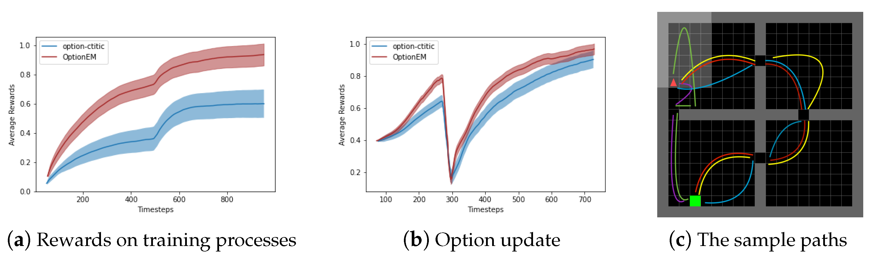
In Figure 2, assuming that options have been provided and are kept fixed throughout the learning process, the only element being updated is the option-value function $Q_{\mathsf{\Omega }}(s,\omega )$. The option policy uses this function for selecting among options. The multi-option update rule from Equation (3) is compared to the case of updating only the sampled option in the state. Four options designed by Sutton et al. are used in this scenario. In this case, the OptionEM method achieves a significantly better sample efficiency, demonstrating how the proposed method accelerates learning the utility of a suitable set of options.

For the case of learning all option parameters, the learning process is conducted using Equation (4). In this setting, the OptionEM method is compared against the option-critic (OC) algorithm and the actor-critic (AC) algorithm. Both the OC and AC algorithms outperform the baseline algorithm in terms of hierarchical agent performance. However, the agent is able to achieve similar performance to the OC algorithm in approximately half the number of episodes. Additionally, it is noteworthy that OptionEM exhibits lower variance across different runs, which is consistent with the anticipated reduction in variance effect of the expected updates from prior research. Figure 2 displays five paths taken by the agent in the game, with fixed start and goal points. Training and exploration processes showcase the comparison experiments between OptionEM and the option-critic algorithm. The option-critic algorithm exhibits some imbalance among options, where a single option is consistently preferred by the policy. This imbalance is more pronounced when using tabular value functions, leading to the degradation of the option-critic algorithm into a regular actor-critic algorithm. However, this imbalance is mitigated when using neural networks for value function approximation. Due to the shared information among options, the robustness of learning strategies on both the environment’s stochasticity and option policy learning process is improved, allowing the OptionEM algorithm to achieve a balanced performance based on state space separation.

The Figure 3 illustrates the option intentions of the OptionEM algorithm and the option-critic algorithm during the testing phase. In order to effectively showcase the learning process of different options, we have chosen to set the game’s background to a white color. In the figure, the green color represents the target location, and the blue portion indicates the current option’s position and distribution. It can be observed that the option-critic algorithm exhibits a noticeable imbalance in the use of options, which might lead to the degradation of the option-critic algorithm into an actor-critic algorithm. The options learned by the OptionEM, using the twin network mechanism, are more balanced compared to the option-critic algorithm. However, there still exists some degradation in option 0 within OptionEM.

4.2. Mujoco

MuJoCo [19] (multi-joint dynamics with contact) is a physics simulator for research and development in robotics, biomechanics, graphics and animation, machine learning, and other fields that require fast and accurate simulation of the interaction of articulated structures with their environment. The default Mujoco games do not effectively demonstrate the subgoal or option characteristics of hierarchical reinforcement learning. Therefore, in this section, the Ant-Maze and Ant-Wall environments are used for training and testing. The Ant-Maze game environment utilizes open-source code from GitHub (environment source code: https://github.com/kngwyu/mujoco-maze.git, accessed on 27 August 2023), while the Ant-Wall game environment is custom-built, featuring randomly initialized walls. In addition to training actions for the ant agent itself, the agent also needs to learn path planning strategies to navigate through mazes or around obstacles/walls. This represents a typical scenario for hierarchical reinforcement learning.

Table 2. MuJoCo game experiment parameters.

	Ant-Maze	Ant-Wall
Learning rate	$2e-4$	$2e-4$
$\gamma$	$0.99$	$0.99$
$\lambda$	$0.95$	$0.95$
$\eta$	$0.95$	$0.95$
Batch size	32	32
Entropy coefficient	$0.0$	$0.0$
Max length	1000	1000

presents the parameter settings for the Mujoco games in this section. When the number of options is set to 2, it is evident that, for both the Ant-Maze and Ant-Wall environments, the agent employs one option when it is far from obstacles/walls and another option when it approaches obstacles/walls. Learning methods based on options provide valuable insights for the agent’s long-term learning/planning in such scenarios.

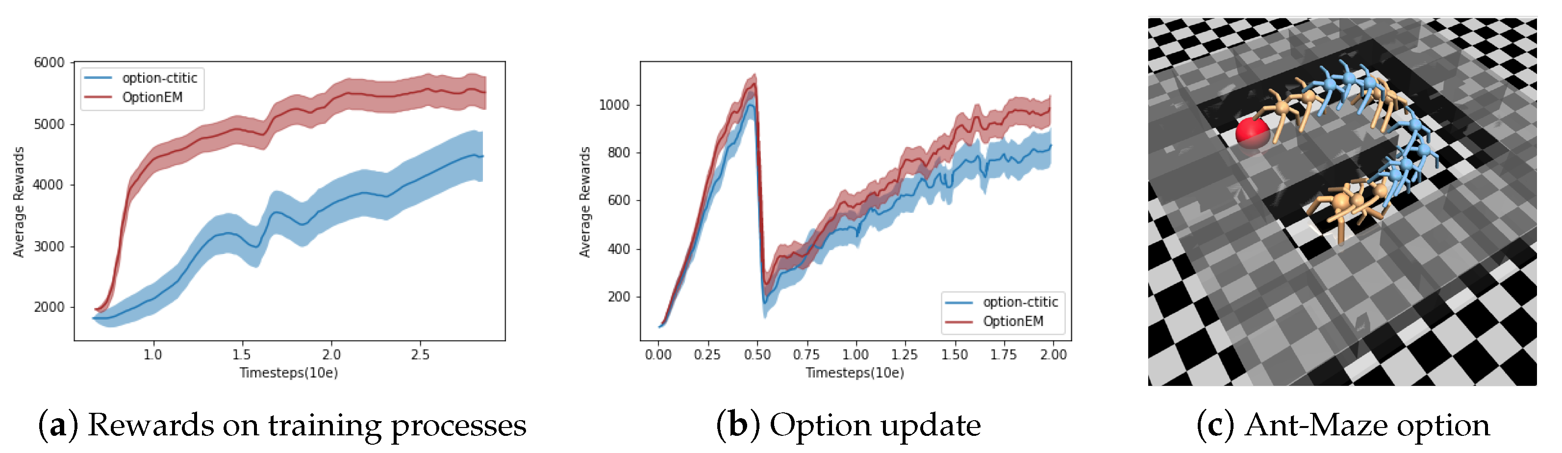
Observing the similarity in path planning between the Ant-Wall and Ant-Corridor games, an attempt was made to transfer the model trained in the Ant-Wall environment to the Ant-Corridor environment. Figure 4 and Figure 5 present the qualitative results of the agent’s learned option categories. In this experiment, the performances from six independent runs were averaged. Additionally, the OptionEM algorithm was compared with two option-based algorithm frameworks, and the results for different numbers of options were compared. In

Table 3. Different numbers of options in Mujoco Ant-Maze game.

Algrithms	2 Options	4 Options	8 Options
OC	$343\left(72\right)$	$291\left(82\right)$	$207\left(61\right)$
Flexible OC	$601\left(93\right)$	$\mathbf{582}\left(\mathbf{73}\right)$	$539\left(86\right)$
OptionEM	$\mathbf{612}\left(\mathbf{110}\right)$	$571\left(102\right)$	$\mathbf{558}\left(\mathbf{97}\right)$

, it is noteworthy that when using eight options the performance eventually drops significantly. This could be attributed to the lower-dimensional environment of the Mujoco experiments and the simplicity of the environment, making such a high number of options unnecessary and decreasing the sample efficiency. One way to validate this is to apply the same algorithm in a continuous learning environment. Furthermore, due to the distinct update rules of the OptionEM algorithm compared to OC baseline and flexible OC algorithms, it can effectively utilize limited sample data, resulting in a better performance.

4.3. UE4-Based Active Tracking

The UE4-based target tracking experiment is mainly designed to verify the generalization of the episodic memory module. A highly realistic virtual environment based on Unreal Engine 4 (UE4) is used for independent learning. The virtual environment has a three-layer structure. The bottom layer consists of simulation scenes based on Unreal 4, which contains a rich variety of scene instances, and provides a general communication interaction interface based on UnrealCV [20], which realizes the communication between the external program and the simulation scene. The agent–environment interaction interface is defined by the specific task, along with the relevant environment elements, such as the reward function, action-state space, etc. The interaction interface design specification is compatible with the OpenAI Gym [21] environment.

The agent actively controls the movement of the camera based on visual observations in order to follow the target and ensure that it appears in the center of the frame at the appropriate size. A successful tracking is recorded only if the camera continues to follow the target for more than 500 steps. During the tracking process, a collision or disappearance of the target from the frame is recognized as a failed tracking. Accurate camera control requires recognition and localization of the target and reasonable prediction of its trajectory. Each time the environment is reset, the camera will be placed anywhere in the environment and the target counterpart will be placed 3 m directly in front of the camera.

The specific tracker reward is as follows:

$$r=A-\left(\frac{\sqrt{x^2+{(y-d)}^2}}{c}+\lambda \left|\omega \right|\right)$$

(18)

For $A>0,c>0,d>0,\lambda >0$, c is set as a normalized distance. The environment defines the maximum reward to a position where the target is directly in front of the tracker (the tracker is parallel to the target character’s shoulders) at a distance of d. With a constant distance, if the target rotates sideways, the tracker needs to turn behind the target to obtain the maximum reward.

In order to enhance the generalization ability of the model, it is necessary to increase the diversity of the surrounding environment and the target itself as much as possible during the training process. In response to the diversity of the surrounding environment, the environment enhancement in UE4 can be used to easily modify the texture, lighting conditions, and other elements of the surrounding environment, specifically, randomly selecting images from a common image dataset deployed on the surface of the environment and objects to modify the texture and randomly deploy the position, intensity, color, and direction of the light source in the environment to change the scene lighting conditions. The randomization of texture and illumination prevents the tracker from overfitting the specific appearance of the target and background. The diversity requirements of the target itself can be realized by varying the target’s trajectory and speed of movement. The start and end position coordinates of the target can be randomly generated, and the corresponding trajectories are generated using the UE4 engine’s built-in navigation module (the trajectories generated by the built-in navigation module automatically avoid obstacles and do not crash into walls). The motion speed of the target is randomly sampled within the range of (0.1 m/s, 1.5 m/s). The randomization of the target motion trajectory and motion velocity allows the bootstrapped sequence encoder to learn the target motion mode and implicitly encode the motion features, avoiding the situation of a single motion pattern. For the training process, at the beginning of each episode, the target character walks along the planned trajectory from a randomly set start position toward the end position, and the tracker starts walking from a position 3 m directly behind the target character, and the tracker needs to adjust the position and camera parameters to make the target always in the center of the tracker screen. For the testing process, the target character’s movement speed is randomly sampled in the range of (0.5 m/s, 1.0 m/s) to test the generalization ability of the model.

The agent is trained and compared with the A3C [22] algorithm adopted by Zhong, Fangwei et al. in the paper [23].The hyper-parameter settings in the experiments are kept the same as in that paper in order to facilitate the comparison. Each game is trained in parallel for six episodes. The seed of the environment is randomly set. The agents are trained from scratch, and, during the training process, the validation is unfolded in parallel. the validation environment is set up in the same way as the training, and the game process with the highest score in the validation environment is selected to report the results for experimental comparison.

An end-to-end conv-lstm network structure is adopted to the tracker agent, which is consistent with the network structure adopted by Luo, Wenhan, Zhong, Fangwei et al. in their paper [23,24]. The convolutional layer and the temporal sequencing layer (LSTM) [25] are not connected by a fully connected layer. The convolutional layer portion uses four layers of convolution and the temporal layer portion uses a single LSTM layer, each containing an ReLU activation layer. The network parameters were updated using the shared Adam optimizer. The observed frame is adjusted to an RGB image of $84\times 84\times 3$ dimensions, which is input to the conv-lstm network, where the convolutional layer extracts features from the input image, and the fully connected layer transforms the feature representation into a 256-dimensional feature vector. Each layer contains a ReLU activation layer. The sequence encoder is a 256-unit single-layer LSTM that encodes the image features temporally. The output of the previous time step is used as part of the input of the next time step, so that the current time step contains the feature information from all previous time steps.

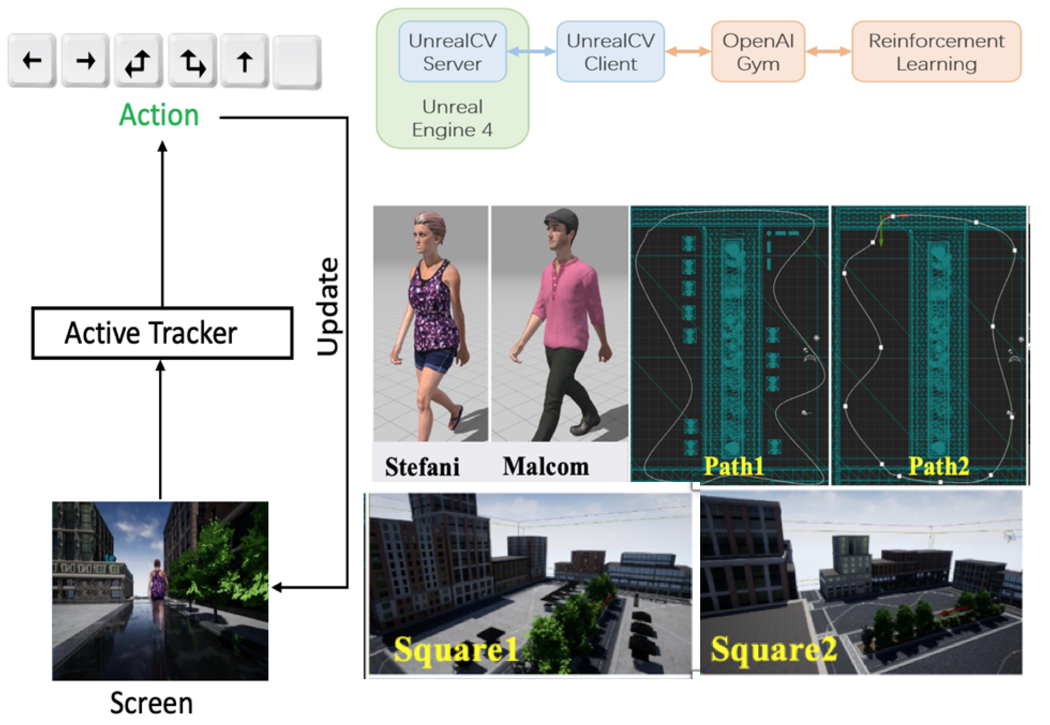
The environment of the tracking game is directly adopted from the environment setting of Zhong, F. et al. in their paper [23], as shown in Figure 6. The game environment consists of a random combination of three elements: character, path, and square.

The effectiveness of the algorithm was tested in four different environments with the combinations S1SP1: Square1StefaniPath1; S1MP1: Square1MalcomPath1; S1SP2: Square1StefaniPath2; and S2MP2: Square2MalcomPath2 and compared with Luo, Wenhan Zhong, Fangwei et al.’s tracker, which was used in their paper [23] (in their paper, the A3C algorithm was used to train the agents).

The comparison experiments were conducted using bootstrappedEM and OptionEM with the A3C method. The options in OptionEM were set to 4 and 8, denoted as OptionEM(4), OptionEM(8), respectively.

Based on the results in

Table 4. Rewards in experiments on UE4 tracking.

Environment	A3C	BootstrappedEM	OptionEM(4)	OptionEM(8)
S1SP1	$2495.7 \pm 12.4$	$2653.1 \pm 2.7$	$\mathbf{2791.4} \mathbf{\pm } \mathbf{20.1}$	$2488.1 \pm 3.0$
S1MP1	$2106.0 \pm 29.3$	$2345.8 \pm 21.6$	$\mathbf{2539.4} \mathbf{\pm } \mathbf{23.1}$	$2142.4 \pm 71.1$
S1SP2	$2162.5 \pm 48.5$	$2401.0 \pm 33.8$	$\mathbf{2519.5} \mathbf{\pm } \mathbf{54.0}$	$2097.3 \pm 45.8$
S2MP2	$740.0 \pm 577.4$	$1624.9 \pm 11.3$	$\mathbf{1741.2} \mathbf{\pm } \mathbf{21.4}$	$1672.4 \pm 42.6$

, the following conclusions can be drawn.

Compared with S1SP1, S1MP1 changes the target role, and all three algorithms perform well on the generalization results of changing the target appearance. Compared with S1SP1, S1SP2 changes the path, and all three algorithms perform well on the generalization result of changing the path. Compared with S1SP1, S2MP2 changes the map, target, and path at the same time, and the generalization results of all three algorithms for this are slightly insufficient compared to the previous two but can still track the target relatively stably, and the model has some generalization potential, which may need to be improved by migration learning or more environmental enhancements. In most cases, the trackers trained by the bootstrappedEM algorithm and the OptionEM algorithm outperform those trained by A3C. The experimental results of the OptionEM(4) algorithm outperformed OptionEM(8), and the performance of the model was instead reduced with eight options, which also indicates that four options is a more appropriate setting in tracking scenarios.

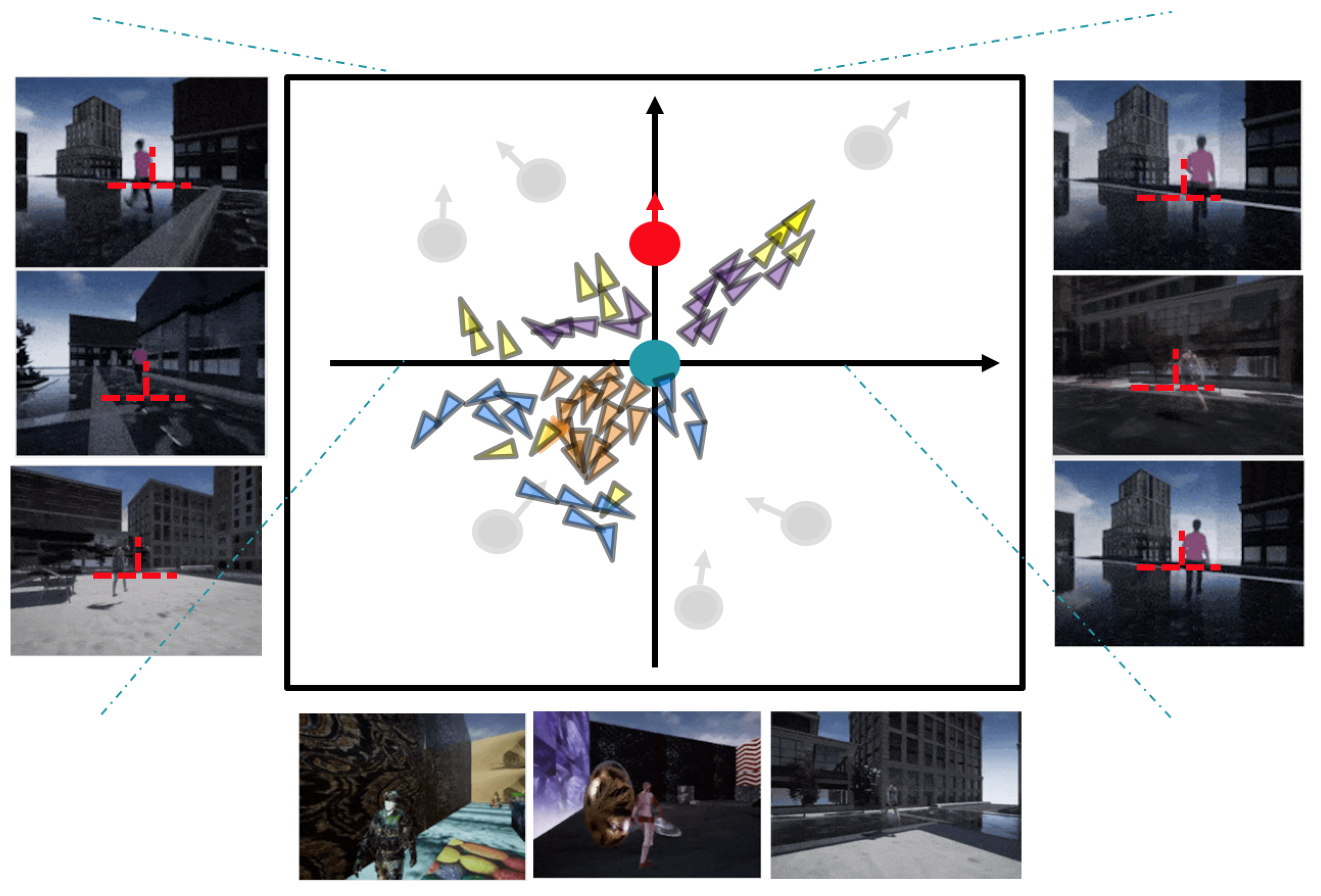
Figure 7 shows the distribution of options learned by the OptionEM algorithm when the number of options is set to four. Observation reveals that the distribution of options can be roughly described as follows: When the target has its back to the tracker and is at a distance, the option with purple marking is selected; when the target has its back to the tracker and is at a closer distance, the option with yellow marking is selected; and when the target is not in the screen or is facing the tracker, there are two possible options. The option with orange marking bootstrapped the tracker to perform a self-rotating motion, while the option with blue marking appears more randomly and the action has no obvious law to be summarized. The model options trained by OptionEM are able to distinguish more clearly between the situation where the target is in the field of view and the situation where the target is lost; when the tracker loses the target in its field of view, the trained options can control the tracker to perform a rotational movement in order to find the lost target as soon as possible. Overall, the distribution of these four options is somewhat consistent with the logic of humans conducting target tracking in real scenes.

Table 5. Training time consumption for UE4-based active tracking.

Baseline	GPU	Time Consumption
A3C	NVIDIA GeForce RTX 2080	2 Days
GEM	NVIDIA GeForce RTX 2080	2 Days
BootstrapEM [26]	NVIDIA GeForce RTX 2080	2 Days
OptionEM	NVIDIA GeForce RTX 2080	28 h

displays OptionEM alongside other baselines in the UE4-based active tracking task, showcasing the time required to train an agent to achieve a cumulative reward of 800. In comparison to the classical A3C algorithm and other episodic memory algorithms, the proposed OptionEM algorithm demonstrates improved efficiency.

5. Summary

In this article, we introduce a hierarchical episodic control model, which employs a hierarchical implicit memory planning approach for value estimation of counterfactual trajectories. The planning process starts from the last step and recursively moves backward along the trajectory, forming an implicit plan in the episodic memory. Experiences are aggregated both along trajectories and across trajectories, and the model is updated using a multi-headed backpropagation mechanism similar to bootstrapped neural networks. This model extends the episodic memory framework to the field of hierarchical reinforcement learning and is theoretically analyzed to demonstrate its convergence and effectiveness.

The results from various experiments, including the four-room game, Mujoco, and UE4 target tracking, indicate that the hierarchical episodic control model effectively enhances training efficiency. It demonstrates significant improvements in both low-dimensional and high-dimensional environments, as well as performing well in sparse environments. Additionally, a summary of the average training times for episodic memory models and hierarchical episodic control models is provided across 57 Atari games and the UE4 tracking game. This summary underscores how the proposed algorithms in this paper can effectively improve training efficiency and reduce the required training time across diverse games and practical applications.

References

1. Botvinick, M.; Ritter, S.; Wang, J.X.; Kurth-Nelson, Z.; Blundell, C.; Hassabis, D. Reinforcement learning, fast and slow. Trends Cogn. Sci. 2019, 23, 408–422. [Google Scholar] [CrossRef] [PubMed]
2. Blundell, C.; Uria, B.; Pritzel, A.; Li, Y.; Ruderman, A.; Leibo, J.Z.; Rae, J.; Wierstra, D.; Hassabis, D. Model-free episodic control. arXiv 2016, arXiv:1606.04460. [Google Scholar]
3. Pritzel, A.; Uria, B.; Srinivasan, S.; Badia, A.P.; Vinyals, O.; Hassabis, D.; Wierstra, D.; Blundell, C. Neural episodic control. In Proceedings of the International Conference on Machine Learning, Sydney, Australia, 6–11 August 2017; pp. 2827–2836. [Google Scholar]
4. Lin, Z.; Zhao, T.; Yang, G.; Zhang, L. Episodic memory deep q-networks. arXiv 2018, arXiv:1805.07603. [Google Scholar]
5. Tulving, E. Episodic memory: From mind to brain. Annu. Rev. Psychol. 2002, 53, 1–25. [Google Scholar] [CrossRef] [PubMed]
6. Tulving, E. What is episodic memory? Curr. Dir. Psychol. Sci. 1993, 2, 67–70. [Google Scholar] [CrossRef]
7. Jing, S. Research on Hierarchical Reinforcement Learning. Ph.D. Thesis, Harbin Engining University, Harbin, China, 2006. [Google Scholar]
8. Bacon, P.L.; Harb, J.; Precup, D. The option-critic architecture. In Proceedings of the AAAI Conference on Artificial Intelligence, San Francisco, CA, USA, 4–9 February 2017; Volume 31. [Google Scholar]
9. Zhang, S.; Whiteson, S. DAC: The double actor-critic architecture for learning options. Adv. Neural Inf. Process. Syst. 2019, 32. [Google Scholar]
10. Savinov, N.; Raichuk, A.; Marinier, R.; Vincent, D.; Pollefeys, M.; Lillicrap, T.; Gelly, S. Episodic curiosity through reachability. arXiv 2018, arXiv:1810.02274. [Google Scholar]
11. Hu, H.; Ye, J.; Zhu, G.; Ren, Z.; Zhang, C. Generalizable episodic memory for deep reinforcement learning. arXiv 2021, arXiv:2103.06469. [Google Scholar]
12. Kulkarni, T.D.; Narasimhan, K.; Saeedi, A.; Tenenbaum, J. Hierarchical deep reinforcement learning: Integrating temporal abstraction and intrinsic motivation. In Proceedings of the Advances in Neural Information Processing Systems, Barcelona, Spain, 5–10 December 2016; pp. 3675–3683. [Google Scholar]
13. Levy, A.; Platt, R.; Saenko, K. Hierarchical actor-critic. arXiv 2017, arXiv:1712.00948. [Google Scholar]
14. Li, A.C.; Florensa, C.; Clavera, I.; Abbeel, P. Sub-policy Adaptation for Hierarchical Reinforcement Learning. arXiv 2019, arXiv:1906.05862. [Google Scholar]
15. Sutton, R.S.; Precup, D.; Singh, S. Between MDPs and semi-MDPs: A framework for temporal abstraction in reinforcement learning. Artif. Intell. 1999, 112, 181–211. [Google Scholar] [CrossRef]
16. Van Hasselt, H.; Guez, A.; Silver, D. Deep reinforcement learning with double q-learning. In Proceedings of the Thirtieth AAAI Conference on Artificial Intelligence, Phoenix, AZ, USA, 12–17 February 2016. [Google Scholar]
17. Chevalier-Boisvert, M.; Dai, B.; Towers, M.; de Lazcano, R.; Willems, L.; Lahlou, S.; Pal, S.; Castro, P.S.; Terry, J. Minigrid & Miniworld: Modular & Customizable Reinforcement Learning Environments for Goal-Oriented Tasks. arXiv 2023, arXiv:2306.13831. [Google Scholar]
18. Klissarov, M.; Precup, D. Flexible Option Learning. Adv. Neural Inf. Process. Syst. 2021, 34, 4632–4646. [Google Scholar]
19. Todorov, E.; Erez, T.; Tassa, Y. Mujoco: A physics engine for model-based control. In Proceedings of the 2012 IEEE/RSJ International Conference on Intelligent Robots and Systems, Vilamoura-Algarve, Portugal, 7–12 October 2012; pp. 5026–5033. [Google Scholar]
20. Qiu, W.; Yuille, A. Unrealcv: Connecting computer vision to unreal engine. In Proceedings of the 14th European Conference on Computer Vision, Amsterdam, The Netherlands, 11–14 October 2016; Springer: Berlin/Heidelberg, Germany, 2016; pp. 909–916. [Google Scholar]
21. Brockman, G.; Cheung, V.; Pettersson, L.; Schneider, J.; Schulman, J.; Tang, J.; Zaremba, W. Openai gym. arXiv 2016, arXiv:1606.01540. [Google Scholar]
22. Mnih, V.; Badia, A.P.; Mirza, M.; Graves, A.; Lillicrap, T.; Harley, T.; Silver, D.; Kavukcuoglu, K. Asynchronous methods for deep reinforcement learning. In Proceedings of the International Conference on Machine Learning, New York, NY, USA, 19–24 June 2016; pp. 1928–1937. [Google Scholar]
23. Luo, W.; Sun, P.; Zhong, F.; Liu, W.; Zhang, T.; Wang, Y. End-to-end active object tracking via reinforcement learning. In Proceedings of the International Conference on Machine Learning, Stockholm, Sweden, 10–15 July 2018; pp. 3286–3295. [Google Scholar]
24. Zhong, F.; Sun, P.; Luo, W.; Yan, T.; Wang, Y. Ad-vat+: An asymmetric dueling mechanism for learning and understanding visual active tracking. IEEE Trans. Pattern Anal. Mach. Intell. 2019, 43, 1467–1482. [Google Scholar] [CrossRef]
25. Hochreiter, S.; Schmidhuber, J. Long short-term memory. Neural Comput. 1997, 9, 1735–1780. [Google Scholar] [CrossRef] [PubMed]
26. Zhou, R.; Wang, Y.; Zhang, X.; Wang, C. Exploration for Countering the Episodic Memory. Comput. Intell. Neurosci. 2022, 2022, 7286186. [Google Scholar] [CrossRef] [PubMed]
Figure 1. Hierarchical implicit memory planning.
Applsci 13 11544 g001
Figure 2. Four-room game experiments.
Applsci 13 11544 g002
Figure 3. Samples of the options in the four-room game.
Applsci 13 11544 g003
Figure 4. Mujoco Ant-Maze game.
Applsci 13 11544 g004
Figure 5. Mujoco Ant-Wall game.
Applsci 13 11544 g005
Figure 6. UE4 environment and settings. Source image: End-to-end Active Object Tracking and Its Real-world Deployment via Reinforcement Learning [23].
Applsci 13 11544 g006
Figure 7. Option samples in UE4 tracking.
Applsci 13 11544 g007