

An Improved Vicsek Model of Swarms Based on a New Neighbor Strategy Considering View and Distance


Abstract
:1. Introduction
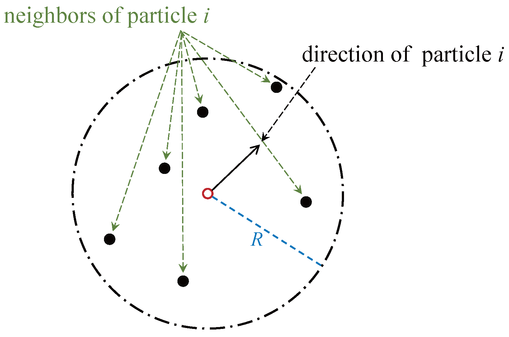
2. The Vicsek Model
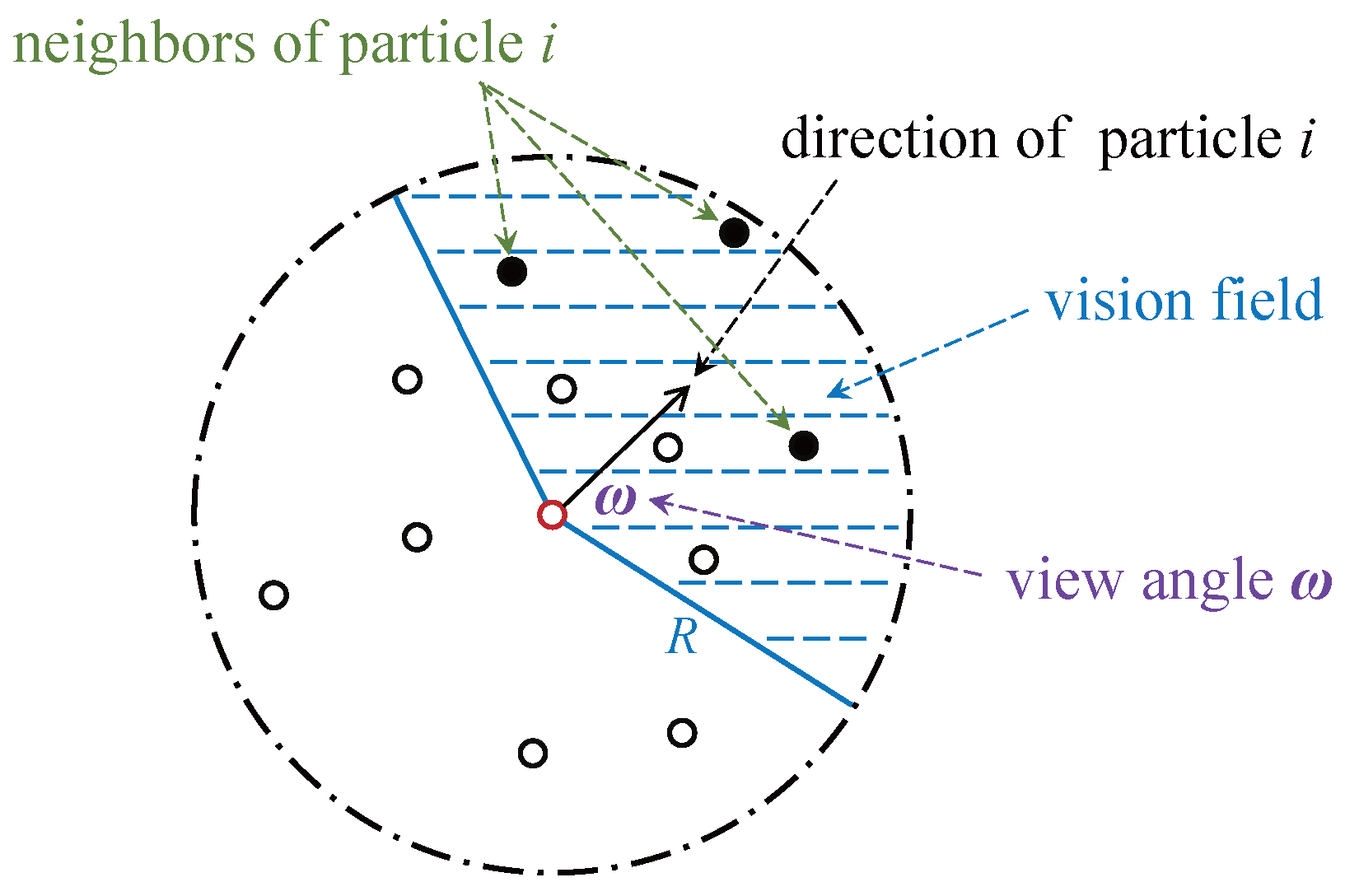
3. The Framework of the Proposed VM
3.1. The Improved SPVM
3.2. The Improved DPVM
4. Simulation and Experiments
4.1. Parameter Settings of Experiments
4.2. Evaluation Indicators of Model Performance
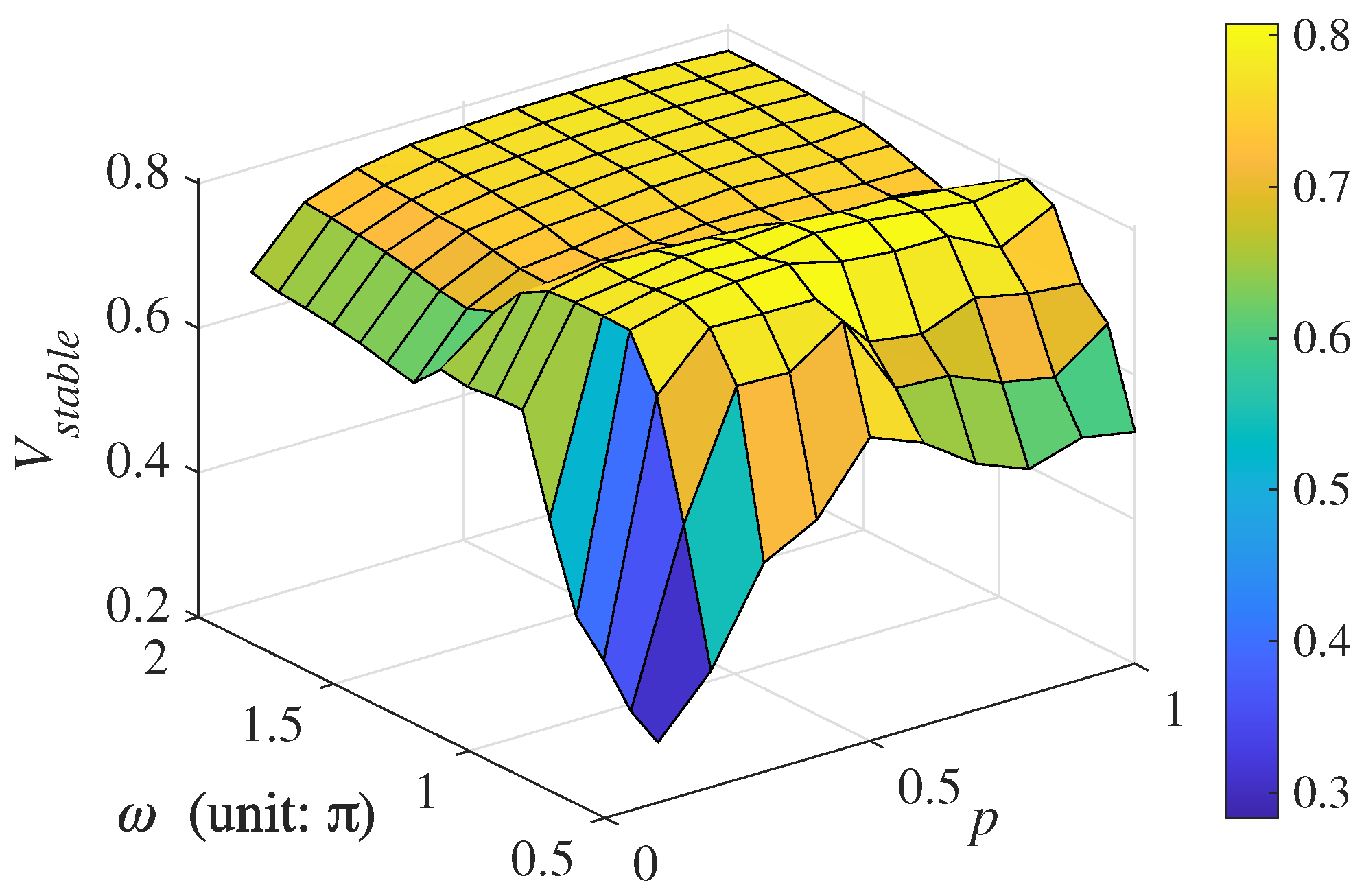
5. Results and Analysis
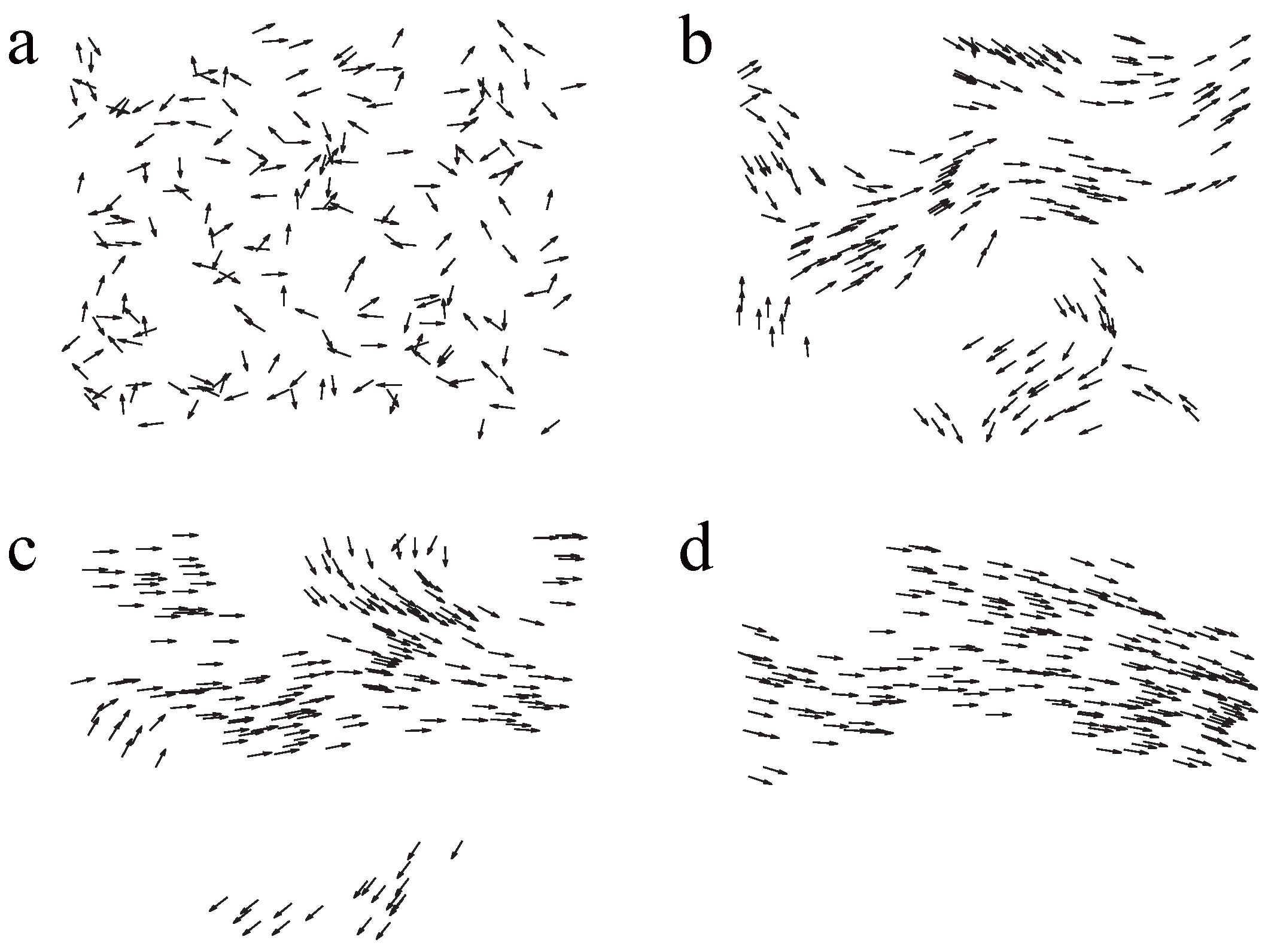
5.1. Simulation and Analysis of SPVM
- Simulation of SPVM under noiseless conditions
- Simulation of SPVM under noisy conditions
- SPVM(1):
- SPVM(2):
- SPVM(3):
- SPVM(4):
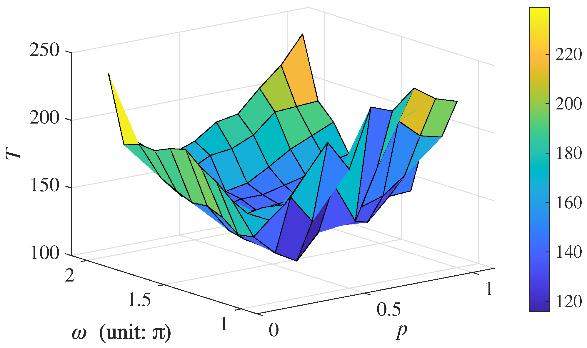
5.2. Simulation and Analysis of DPVM
6. Conclusions
Author Contributions
Funding
Institutional Review Board Statement
Informed Consent Statement
Data Availability Statement
Conflicts of Interest
References
- Attanasi, A.; Cavagna, A.; Del Castello, L.; Giardina, I.; Melillo, S.; Parisi, L.; Pohl, O.; Rossaro, B.; Shen, E.; Silvestri, E.; et al. Collective behaviour without collective order in wild swarms of midges. PLoS Comput. Biol. 2014, 10, e1003697. [Google Scholar] [CrossRef] [PubMed]
- Buhl, J.; Sumpter, D.J.T.; Couzin, I.D.; Hale, J.J.; Despland, E.; Miller, E.R.; Simpson, S.J. From disorder to order in marching locusts. Science 2006, 312, 1402–1406. [Google Scholar] [CrossRef] [PubMed]
- Bialek, W.; Cavagna, A.; Giardina, I.; Mora, T.; Silvestri, E.; Viale, M.; Walczak, A.M. Statistical mechanics for natural flocks of birds. Proc. Natl. Acad. Sci. USA 2012, 109, 4786–4791. [Google Scholar] [CrossRef] [PubMed]
- Bode, N.W.F.; Franks, D.W.; Wood, A.J. Limited interactions in flocks: Relating model simulations to empirical data. J. R. Soc. Interface 2011, 8, 301–304. [Google Scholar] [CrossRef] [PubMed]
- Herbert-Read, J.E.; Perna, A.; Mann, R.P.; Schaerf, T.M.; Sumpter, D.J.T.; Ward, A.J.W. Inferring the rules of interaction of shoaling fish. Proc. Natl. Acad. Sci. USA 2011, 108, 18726–18731. [Google Scholar] [CrossRef] [PubMed]
- Katz, Y.; Tunstrøm, K.; Ioannou, C.C.; Huepe, C.; Couzin, I.D. Inferring the structure and dynamics of interactions in schooling fish. Proc. Natl. Acad. Sci. USA 2011, 108, 18720–18725. [Google Scholar] [CrossRef] [PubMed]
- Hu, W.; Wen, G.; Rahmani, A.; Bai, J.; Yu, Y. Leader-following consensus of heterogenous fractional-order multi-agent systems under input delays. Asian J. Control 2020, 22, 2217–2228. [Google Scholar] [CrossRef]
- Innocente, M.; Grasso, P. Self-organising swarms of firefighting drones: Harnessing the power of collective intelligence in decentralised multi-robot systems. J. Comput. Sci. 2019, 34, 80–101. [Google Scholar] [CrossRef]
- Li, R.; Xiong, Y.; Zhang, T. Intelligent path planning algorithm for UAV group based on machine learning. J. Phys. Conf. Ser. 2021, 1865, 042118. [Google Scholar] [CrossRef]
- Ahad, M.A.; Ahmad, S.M. Investigation of a 2-DOF active magnetic bearing actuator for unmanned underwater vehicle thruster application. Actuators 2021, 10, 79. [Google Scholar] [CrossRef]
- Kim, J. Underwater guidance of distributed autonomous underwater vehicles using one leader. Asian J. Control 2022, 25, 2641–2654. [Google Scholar] [CrossRef]
- Reynolds, C.W. Flocks, herds and schools: A distributed behavioral model. ACM Siggraph Comput. Graph. 1987, 21, 25–34. [Google Scholar] [CrossRef]
- Vicsek, T.; Czirók, A.; Ben-Jacob, E.; Cohen, I.; Shochet, O. Novel type of phase transition in a system of self-driven particles. Phys. Rev. Lett. 1995, 75, 1226–1229. [Google Scholar] [CrossRef]
- Chaté, H. Dry Aligning Dilute Active Matter. Annu. Rev. Condens. Matter Phys. 2020, 11, 189–212. [Google Scholar] [CrossRef]
- Cai, L.B.; Chaté, H.; Ma, Y.Q.; Shi, X.Q. Dynamical subclasses of dry active nematics. Phys. Rev. E 2019, 99, 010601. [Google Scholar] [CrossRef]
- Ben-Jacob, E.; Shochet, O.; Tenenbaum, A.; Cohen, I.; Czirók, A.; Vicsek, T. Response of bacterial colonies to imposed anisotropy. Phys. Rev. E 1996, 53, 1835–1843. [Google Scholar] [CrossRef]
- Geiß, D.; Kroy, K.; Holubec, V. Signal propagation and linear response in the delay Vicsek model. Phys. Rev. E 2022, 106, 054612. [Google Scholar] [CrossRef]
- Serna, H.; Góźdź, W.T. The influence of obstacles on the collective motion of self-propelled objects. Phys. Stat. Mech. Appl. 2023, 625, 129042. [Google Scholar] [CrossRef]
- You, F.; Yang, H.X.; Li, Y.; Du, W.; Wang, G. A modified Vicsek model based on the evolutionary game. Appl. Math. Comput. 2023, 438, 127565. [Google Scholar] [CrossRef]
- Shang, L.; Xu, Z. Adaptive control strategy improves synchronization of self-propelled agents. Appl. Math. Comput. 2023, 454, 128102. [Google Scholar] [CrossRef]
- González-Albaladejo, R.; Carpio, A.; Bonilla, L.L. Scale-free chaos in the confined Vicsek flocking model. Phys. Rev. E 2023, 107, 014209. [Google Scholar] [CrossRef] [PubMed]
- Chatterjee, S.; Mangeat, M.; Woo, C.U.; Rieger, H.; Noh, J.D. Flocking of two unfriendly species: The two-species Vicsek model. Phys. Rev. E 2023, 107, 024607. [Google Scholar] [CrossRef] [PubMed]
- Zhang, X.; Fan, S.; Wu, W. Enhancing synchronization of self-propelled particles via modified rule of fixed number of neighbors. Phys. Stat. Mech. Appl. 2023, 629, 129203. [Google Scholar] [CrossRef]
- Xue, T.; Li, X.; Grassberger, P.; Chen, L. Swarming transitions in hierarchical societies. Phys. Rev. Res. 2020, 2, 042017. [Google Scholar] [CrossRef]
- Lu, X.; Zhang, C.; Huang, C.; Qin, B. Research on swarm consistent performance of improved Vicsek model with neighbors’ degree. Phys. A 2022, 588, 126567. [Google Scholar] [CrossRef]
- Gao, J.; Chen, Z.; Cai, Y.; Xu, X. Enhancing the convergence efficiency of a self-propelled agent system via a weighted model. Phys. Rev. E 2010, 81, 041918. [Google Scholar] [CrossRef]
- Chen, Y.R.; Zhang, X.X.; Yu, Y.S.; Ma, S.W.; Yang, B. Enhancing convergence efficiency of self-propelled agents using direction preference. Phys. A 2022, 586, 126415. [Google Scholar] [CrossRef]
- Li, W.; Wang, X. Adaptive velocity strategy for swarm aggregation. Phys. Rev. E 2007, 75, 021917. [Google Scholar] [CrossRef]
- Tian, B.M.; Yang, H.X.; Li, W.; Wang, W.X.; Wang, B.H.; Zhou, T. Optimal view angle in collective dynamics of self-propelled agents. Phys. Rev. E 2009, 79, 052102. [Google Scholar] [CrossRef]
- Zhang, X.; Jia, S.; Li, X. Improving the synchronization speed of self-propelled particles with restricted vision via randomly changing the line of sight. Nonlinear Dyn. 2017, 90, 43–51. [Google Scholar] [CrossRef]
- Lu, X.; Zhang, C.; Qin, B. An improved Vicsek model of swarm based on remote neighbors strategy. Phys. A 2022, 587, 126553. [Google Scholar] [CrossRef]
- Martin, G. Visual fields in woodcocks Scolopax rusticola (Scolopacidae; Charadriiformes). J. Comp. Physiol. A-Neuroethol. Sens. Neural Behav. Physiol. 1994, 174, 787–793. [Google Scholar] [CrossRef]
- Bajec, I.L.; Heppner, F.H. Organized flight in birds. Anim. Behav. 2009, 78, 777–789. [Google Scholar] [CrossRef]
- Wang, X.G.; Zhu, C.P.; Yin, C.Y.; Hu, D.S.; Yan, Z.J. A modified Vicsek model for self-propelled agents with exponential neighbor weight and restricted visual field. Phys. A Stat. Mech. Its Appl. 2013, 392, 2398–2405. [Google Scholar] [CrossRef]


| Category | Method |
|---|---|
| Providing more information | Hierarchical society [24], Neighbors’ degree [25] |
| Weight difference [26], Direction preference [27] | |
| Adaptive velocity [28] | |
| Providing less information | Evolutionary game theory [19], Line of sight [30] |
| RVFVM [29], RNSVM [31] | |
| The proposed new neighbor strategy |
| SPVM(1) | SPVM(4) | DPVM | |
|---|---|---|---|
| 0.7783 | 0.8032 | 0.7973 | |
| 55 | 1579 | 96 |
Disclaimer/Publisher’s Note: The statements, opinions and data contained in all publications are solely those of the individual author(s) and contributor(s) and not of MDPI and/or the editor(s). MDPI and/or the editor(s) disclaim responsibility for any injury to people or property resulting from any ideas, methods, instructions or products referred to in the content. |
© 2023 by the authors. Licensee MDPI, Basel, Switzerland. This article is an open access article distributed under the terms and conditions of the Creative Commons Attribution (CC BY) license (https://creativecommons.org/licenses/by/4.0/).
Share and Cite
Wang, X.; Zhao, H.; Li, L. An Improved Vicsek Model of Swarms Based on a New Neighbor Strategy Considering View and Distance. Appl. Sci. 2023, 13, 11513. https://doi.org/10.3390/app132011513
Wang X, Zhao H, Li L. An Improved Vicsek Model of Swarms Based on a New Neighbor Strategy Considering View and Distance. Applied Sciences. 2023; 13(20):11513. https://doi.org/10.3390/app132011513
Chicago/Turabian StyleWang, Xiaocheng, Hui Zhao, and Li Li. 2023. "An Improved Vicsek Model of Swarms Based on a New Neighbor Strategy Considering View and Distance" Applied Sciences 13, no. 20: 11513. https://doi.org/10.3390/app132011513
APA StyleWang, X., Zhao, H., & Li, L. (2023). An Improved Vicsek Model of Swarms Based on a New Neighbor Strategy Considering View and Distance. Applied Sciences, 13(20), 11513. https://doi.org/10.3390/app132011513