Observing Material Properties in Composite Structures from Actual Rotations

Abstract

The shear deflection effects are traditionally neglected in most structural system identification methods. Unfortunately, this assumption might lead to significant errors in some structures, like deep beams. Although some inverse analysis methods based on the stiffness matrix method, including shear deformation effects, have been presented in the literature, none of these methods are able to deal with actual rotations in their formulations. Recently, the observability techniques, one of the first methods for the inverse analysis of structures, included the shear effects into the system of equations. In this approach, the effects of the shear rotation are neglected. When actual rotations on-site are used to estimate the mechanical properties in the inverse analysis, it can result in serious errors in the observed properties. This characteristic might be especially problematic in structures such as deep beams where only rotations can be measured. To solve this problem and increase the observability techniques’ applicability, this paper proposes a new approach to include the shear rotations into the inverse analysis by observability techniques. This modification is based on the introduction of a new iterative process. To illustrate the applicability and potential of the proposed method, the inverse analysis of several examples of growing complexity is presented.

1. Introduction

Structural modeling is associated with the simulation of a structural response. This goal is traditionally achieved by transforming physical problems into mathematical ones based on a number of assumptions and hypotheses. Many studies are performed on the model of the beam structural response [1,2,3,4] and most of them are based on either Euler–Bernoulli’s beam theory [5] or Timoshenko’s beam theory (known as first-order shear deformation theory) [6]. Due to the plain section deformation assumption, shear deformations are neglected by Euler–Bernoulli’s beam theory [7,8]. This theory states that plane sections remain perpendicular to the neutral axis during and after bending deformation [9], and accordingly that shear forces and stresses are zero. Euler–Bernoulli’s beam theory only holds for cases wherein constant bending moments are applied alongside the structures. Therefore, Euler–Bernoulli’s beam theory is usually applied to slender beams with negligible shear deformations and in this approach, shear effects are considered modeling errors [10]. Nevertheless, in some structures (such as deep beams), the shear deformation cannot be neglected and it must be included into the formulation [11,12]. The definition of these deep beams might differ slightly from one code to the other. For example, on the one hand, Eurocode EN 1992-1-1 [13] characterizes deep beams as beams having a slenderness ratio where the span of the beam is one third or less of the total section depth. On the other hand, the ACI committee 318 [14] describes these beams as beams with spans equal to or less than four times the beam’s depth.

Timoshenko [15] was the first one who introduced the shear effects into beams with the so-called first-order shear deformation theory. It is a widely used engineering theory for analyzing the behavior of beams that are subjected to bending and shearing loads. The Timoshenko theory is particularly useful for analyzing beams that are relatively thin, long, or have open cross-sections, where shear deformation effects are more pronounced. It is often applied to problems involving beams in aerospace, civil, and mechanical engineering. This theory can handle a wide range of boundary conditions and loading scenarios, making it suitable for various practical engineering applications. Unlike the simpler Euler–Bernoulli beam theory, which neglects shear deformation, the Timoshenko theory considers both bending and shearing effects in the analysis of beams. The theory incorporates the effects of shear deformation, which means it considers the change in the angle of the cross-section during bending. In contrast, the Euler–Bernoulli theory assumes that cross-sections remain perpendicular to the longitudinal axis of the beam. In fact, unlike Euler–Bernoulli’s beam theory which only considers bending rotations (w_b), in Timoshenko’s beam theory (known as Timoshenko’s beam theory or first-order shear deformation theory) rotation due to the bending, w_b, and rotation due to the shear, w_r are considered separately and analyzed independently. In this theory, rotation between the cross-section and the bending line is allowed. The differences between methods in a simply supported beam with concentrated load, V, at the mid-span are presented in Figure 1, where Euler–Bernoulli’s beam theory (Figure 1b) and Timoshenko’s beam theory (Figure 1c) at the zoomed support of Figure 1a can be seen.

The finite element method (FEM) is a numerical technique employed in engineering and computational science to solve partial differential equations and simulate physical phenomena. This approach entails the subdivision of a complex problem or domain into smaller, more manageable subdomains or elements, with the approximation of the solution within each element. This technique is a common method for computer-based analysis in engineering [16]. The stiffness matrix method (SMM) is one of the major methods of the FEM approach for analyzing the structural response of beam-like structures. The literature review showed that a number of SMM approaches included shear rotation into their SMM formulations [17,18,19,20,21,22]. However, most of these methods fail to simulate structural cases with discontinuities in the cross-sections, with non-collinear elements, or with non-uniform loads. The only SMMs that are able to analyze these models are the FEMs in which nodal variables are the bending rotation and transverse displacement (the effects of shear rotation are neglected in this SMM formulation). Many works, for instance in Przemieniecki [23], contain a detailed formulation of the common Timoshenko beam theory SMM. The stiffness matrix presented in this approach overlooks the effect of the shear rotation. Emadi [24] highlighted the neglect of the shear rotation effects in some widely used commercial simulation software that rely on the stiffness matrix, such as SAP 2000, CSI 2016, and Midas Civil 2015. In fact, these programs only include the shear effects into the vertical deflections. However, it has been traditionally assumed that shear rotations have minimal practical significance in most structures. This assumption can introduce significant errors in the determination of the mechanical properties during the inverse analysis of structures that lack a unidimensional geometry, such as deep beams, laminated composite walls, or sandwich structures. In such cases, shear deformation can play a crucial role, and it is essential to incorporate its effects into the formulation.

System identification (SI) represents a modeling process for unknown variables in a certain system of equations used in numerous engineering fields [25,26,27]. The SI goal is to be able to characterize adequately the parameters of a certain system. Since its introduction, SI has been extended to most engineering fields [18,28]. Structural system identification (SSI) can be framed in the context of the SI that deals with the design of mathematical models for identifying structural parameters (such as the flexural or the axial stiffnesses) [29]. In the literature, many methods for SSI are proposed. Most of them are based on the SMM (see, e.g., [30,31,32,33,34]). The details of the main SSI methods are shown in the literature and addressed by [35]. Most SSI methods are not able to quantify correctly the structural parameters when shear effects are not negligible. This can be explained by the fact that most SSI methods based on SMM normally use Euler–Bernoulli’s beam theory (see, e.g., [36,37,38]), this assumption underestimates deflections and overestimates the natural frequencies since the shear effects are disregarded [39]. The effects of shear deformations in their SMM models are studied by some authors [8,40]. Although the assumption of neglecting shear rotations may lead to wrong estimations for mechanical properties in SSI methods, normally these effects are overlooked. Nevertheless, in some structures (such as deep beams) shear effects might play an important role. In these cases, shear effects should be introduced into the formulation in order to reduce the errors of SSI methods, and the inability of considering these effects should be considered a modeling error (error in the modeling of structures).

The observability method (OM) is an SSI method based on the system of equations of the SMM. In this procedure, the mechanical properties (e.g., flexural stiffness, EI) can be quantified from the deformations measured in static tests. The OM has proved its efficiency in different structural typologies (such as trusses, beams, frame structures, and cable-stayed bridges) [41,42]. The analysis of these structures is based on polynomial systems of equations, and it is not as simple as it may look due to the coupled equations. To solve this problem, a numerical optimization approach (constrained observability method (COM)) can be used to decouple the coupled linearized variables. Recently, Emadi et al. [43] included the effects of shear deformations into the COM. Unfortunately, this application (like other SSI methods based on SMM in the literature) is not able to take into account the actual rotations as the shear rotation effects are not included into the formulation. Because of the inability of this method to consider shear rotations in SMM, the COM is not able to observe the value of the mechanical properties correctly, when actual rotations are included into the measurement sets. For this reason, this procedure is not suitable for actual structures as wrong results are obtained even when noise-free measurements are considered.

This paper aims to fill this gap by presenting a new method based on the COM to observe the structural properties from the actual rotations measured on-site for any kind of structure (even in those where shear rotations are not negligible). To do so, the use of an iterative process is proposed. In this process, estimated shear rotations are subsequently subtracted from the actual rotations on site. Then, the normal COM can be performed in terms of bending rotations and bending and shear vertical deflections. Also, throughout iterative steps, the structural properties are successively updated from the inverse observations.

This article is organized as follows: In Section 2, a brief explanation of both the OM and the COM are presented and the importance of shear rotation is discussed. Also, a new method for analyzing the effects of the shear rotation in the COM is presented. In Section 3, different structures are analyzed to show the important role that shear rotations might play in some geometries. Moreover, the applicability and accuracy of the new method in different structures are presented. Finally, the conclusions obtained are drawn in Section 4.

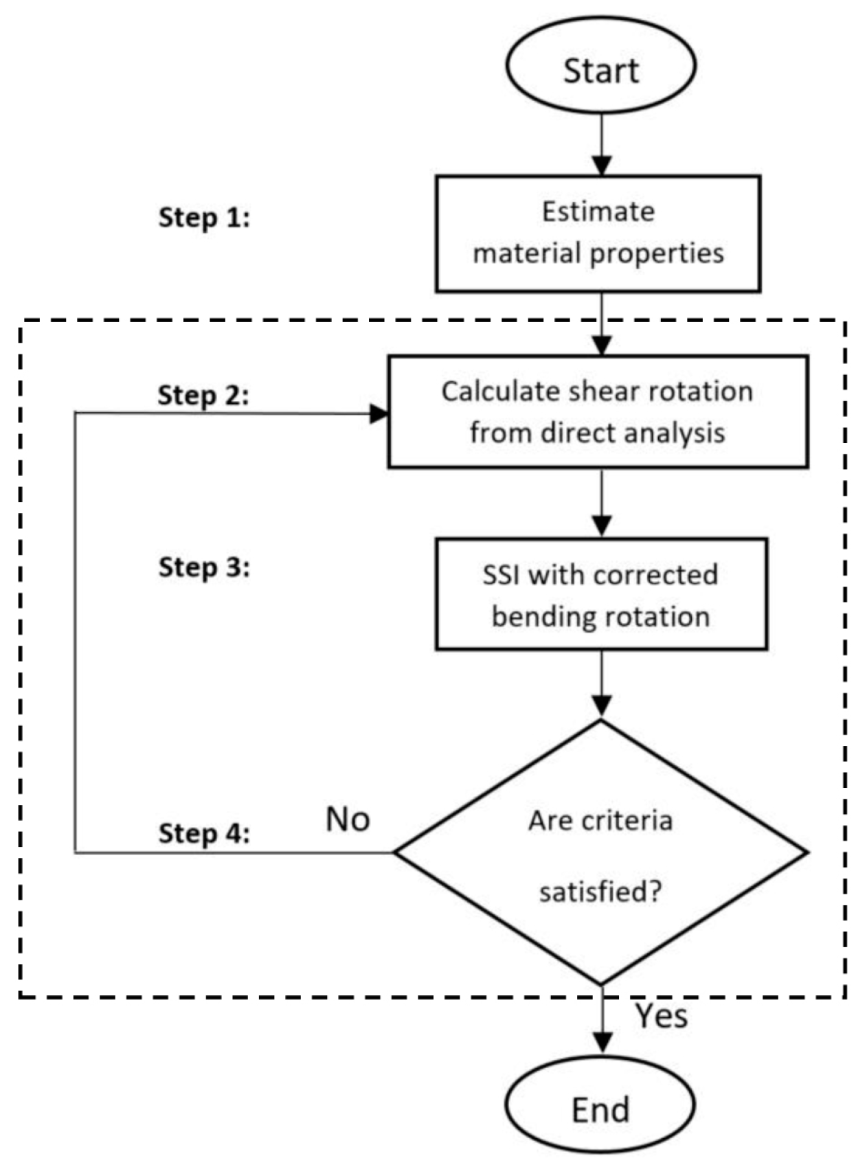
2. Materials and Methods

For the SMM, the equations of nodal equilibrium might be written as:

$$\left[\mathrm{K}\right]\cdot \{\delta \}=\{\mathrm{f}\},$$

(1)

where the horizontal u, vertical v, and rotational displacements w, are parts of {δ}, the stiffness matrix [K] covers information about axial stiffness EA, flexural stiffness EI, and the length of the element L. The horizontal forces, vertical forces, and moments are included in the external force vector {f}.

The main disadvantage of this method is that the complexity in the system of equations might lead to the following problems: (1) They are not able to include the effect of shear rotation into the SMM methods, so these methods are considered as common Timoshenko’s beam theory SMM (e.g., [23]). (2) Methods which consider the effects of shear rotation due to some assumptions, are not applicable in general complex structures [44]. In the OM, as in any inverse tool, some parameters of the nodal displacements {δ} are measured on-site to identify the unknown mechanical properties in the SMM when the geometry, the boundary conditions, and the load case in a certain static load test are determined. To do so, Equation (1) can be rewritten as presented in Equation (2), where all the known quantities are collected into the coefficient matrix [B] and the vector {D}. Therefore, [B] and {D} are known, while all the unknowns are placed into the vector {Z}. Equation (2) can be solved to observe unknown equations with the help of algebraic operations. For more information, readers are recommended to read [42].

$$\left[\mathrm{B}\right]\cdot \{z\}=\{\mathrm{D}\},$$

(2)

In the OM, the system is assumed to be linear, and coupled products of variables are considered single variables (such as Young’s modulus E, and inertia I are considered as a unique variable EI). Here, N_A is the unknown axial stiffnesses and N_F is the unknown flexural stiffnesses. Theoretically, the number of measurements should be at least equal to the number of unknowns; therefore, N_A + N_F measurements are expected to be enough to observe all unknown parameters. Lei et al. [42] found that due to the lack of nonlinear constraints among product variables in OM, in most cases, it is not able to observe the material properties with the minimum required measurements. Lei et al. [42] proposed a COM which solves the system of equations numerically after including the nonlinear constraints. This is to say that the COM does not provide any symbolic solution, as they are only based on the numerical solution of the system. In order to apply the optimization process, the objective function of the COM can be defined as follows:

$$\left\{\epsilon \right\}=\left[B\right]·\left\{Z\right\}-\left\{D\right\},$$

(3)

where {ε} is the residual of the equations which is a vector with the same number of rows as the original vector {Z}. The objective function of the optimization process is to minimize the square sum of the residuals, ε in Equation (3). MATLAB and Optimization Toolbox Release [45] are used to obtain the optimal solution of the objective function. Before starting the optimization process, the objective function should be normalized. The algorithm for SSI by COM is summarized as follows:

Step 1: Apply SSI by OM to check whether any variable is observed. If all unknown parameters are observed, there is no need to go to the COM process, otherwise, go to step 2.

Step 2: Obtain Equation (2) from the OM and generate the objective function.

Step 3: Obtain the normalized unknown parameters.

Step 4: Guess the unknown parameters’ initial values, apply bounds for the solution and solve the optimization process, in order to find the least acceptable value for vector {ε}.

A summary of the procedure is shown in the flow chart in Figure 2. For more information about the COM, the reader is directed to [42].

Since the COM method was based on Euler–Bernoulli’s SMM, it was not able to consider the effects of shear deflections. This problem was solved by Emadi et al. [43], who introduced the effects of shear deformation into the COM process. Due to a lack of considering the shear rotation in SMM, COM is not able to observe the value of the material properties correctly when rotations are included into the measurement sets. This method is not suitable for measuring rotations as wrong results are obtained even in noise-free measurements when these types of deformations are considered. Emadi studied the effects of this impotence in considering the shear rotations in SSI methods based on SMM [44]. It showed the effects of neglecting the shear rotation in the inverse analysis were not negligible, even in the cases where beams cannot be considered deep beams (based on Eurocode EN [13] and by the ACI Committee 318 [14]).

In this section, a new procedure is developed to take into account the effects of shear rotations in the SSI of two-dimensional structures modeled with beam elements.

Providing that a static load test is performed in a structure and measurements are taken from some nodal displacements (total deflections and rotations including bending and shear displacements and rotations), the first step will be trying to separate the bending and shear rotations. Then, the direct analysis is performed assuming those beam elements have their theoretical mechanical properties. Then, the shear rotation of each element is calculated based on the assumed mechanical properties. Equation (4) can be used to calculate shear rotation vs. in each element based on Timoshenko’s beam theory.

$${\mathrm{W}}_{\mathrm{s}}=\frac{Q}{A_v\ast G}$$

(4)

where A_v is the shear area, Q is the shear force, and the shear modulus G might be written as:

$$\mathrm{G}=\frac{\mathrm{E}}{2(1+\mathrm{v})}$$

(5)

where the coefficient v refers to the Poisson’s ratio. According to Equation (4), the shear rotation for each element only depends on shear forces, shear area, and shear modulus. On the other hand, shear area and shear modulus are directly obtained from the assumed mechanical properties of the structure, while the shear forces can be obtained from the results of the direct SMM analysis. By subtracting the value of shear rotation from the measured rotation of each node the bending rotation can be obtained (it is important to highlight that the measured rotation can be expressed as the sum of shear and bending rotations). Therefore, the COM process can be used as it is based on neglecting the shear rotation effects. Once COM provides an estimate of the mechanical properties of the structure, these can be used to calculate new shear rotations. In this way, an iterative process should be performed until the adequate structural response of all the elements is satisfied. In order to limit the computational cost of the optimization process, the stopping criteria are defined: (1) when the iterative process is performed more than 200 times without leading to an improvement of the solution, and (2) when the difference between the values of the observed structural properties in 2 subsequent iterative steps are less than 1 × 10⁻³.

The main steps of this procedure are described as follows:

Step 1: Assume the initial values of the structural properties as the theoretical ones

Step 2: Calculate the shear rotation of each element from the assumed structural properties and static loads. It is important to highlight that the stiffness properties can be obtained through either theoretical values (for the first time) or observed structural properties provided by the COM optimization (in the iterative process).

Step 3: Obtain the bending rotation from the calculated shear rotation in Step 2 and perform COM analysis. The value of the bending rotation for the measured nodes is calculated by subtracting the actual value (measured on-site) from the theoretical shear rotation calculated in Step 2.

Step 4: Check the stopping criteria. If one of them is satisfied, the process stops, otherwise, go to Step 2.

A summary of the procedure is shown in the flow chart in Figure 3. In the following section, a set of structures are analyzed to illustrate the applicability and potential of the proposed method. This will be called 2COM as COM is applied in two steps.

3. Results

To show the applicability of the new method, several demonstrative examples are analyzed in this section. It is important to highlight that in these simulations, no horizontal forces are considered, and therefore the axial resistant mechanisms are not studied as they are not excited. In addition, measurement errors are neglected in the simulations.

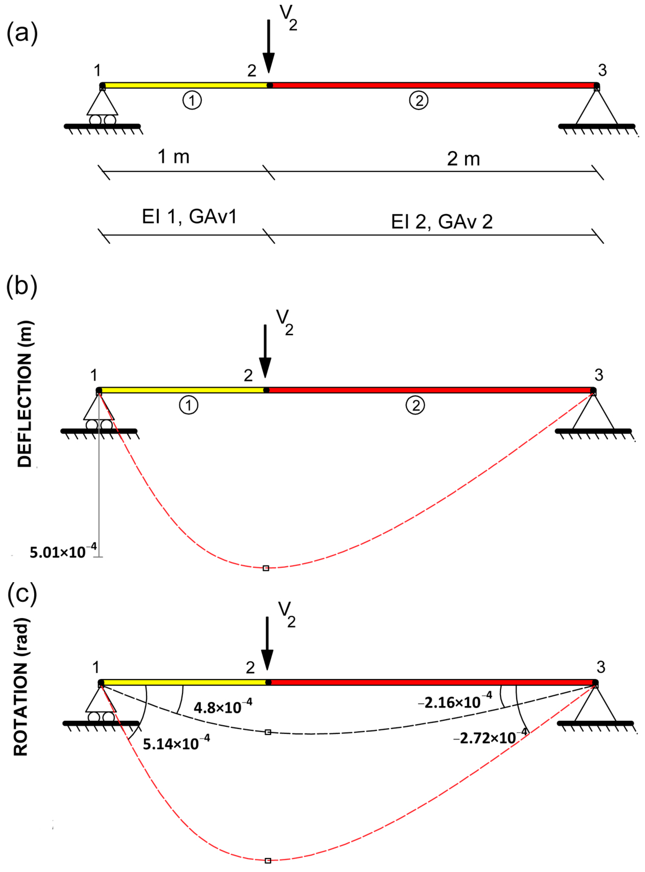
3.1. Example 1: Simply Supported Beam with Two-Iteration Processes

Consider the 3-m long and 0.2-m wide simply supported beam modeled with three nodes and two beam elements depicted in Figure 4a. A deformed shape with the value of bending vertical deformation and with bending and shear vertical deformation at node 2 can be seen in Figure 4b and a deformed shape with bending rotation and with bending and shear rotation at node 1 is illustrated in Figure 4c. This beam has a rectangular constant cross-section with a 1m² cross-sectional area. Its mechanical properties are listed in

Table 1. Properties of the FEM of the simply supported beam.

Properties	Value
axial stiffness [GPa·m2]	440.65
shear stiffness for node 1 [GPa·m2]	344.05
shear stiffness for node 2 [GPa·m2]	385
flexural stiffness for node 1 [GPa·m4]	1246.7
flexural stiffness for node 2 [GPa·m4]	1120

. The boundary conditions of the structure are horizontal and vertical displacements restricted in node 3 and vertical displacement is restricted in node 1 (this is to say v₁ = u₃ = v₃ = 0). The beam is subjected to a concentrated vertical force in node 2 of 100 kN (V₂ = 100 kN).

For the inverse analysis of the structure, the load V₂, the length of the elements, Poisson’s ratio, and Young’s modulus E are assumed as known, while the inertia I, and the shear area A_v for both elements are assumed as unknown. To identify the two unknown parameters (A_v and I) a measurement set of at least four rotations is required to identify the values of the unknowns. As explained in Section 2, the COM is based on the optimization application, therefore, all variables are always observed. Regardless of their accuracy. In order to ensure the reliability of the COM-based model, it is advised to perform a traditional OM which is based on the linear equation. The analysis of the traditional OM of this model proves that no set of four rotations in the OM enables the proper identification of the unknown parameters. Therefore, a set of vertical deflection and a rotation should be measured together (it is to say w₁, w₂, w₃ and v₂). The values of the measurement set obtained from Timoshenko’s beam theory simulation can be seen in Figure 4b,c.

To check the robustness of the method, a set of random values is chosen for the inertia and shear area to be used to calculate the hypothetical site measurements. A total of 50 different random sets of the initial value coefficients for the inertia and the shear area were randomly chosen between 0.8 and 1.2 of the theoretical values. These initial parameters are successively updated throughout the iterative process. From 50 analyses, in three analyses the optimization process was not convergent to the solution and no result was acquired. The normalized average, standard deviation, and coefficient of variation of the remaining results as well as the mode are presented in

Table 2. Obtained results from random initial values of example 1.

Parameter	Average	CoV	Standard Deviation
EI1	1.000	8.791 × 10−7	8.791 × 10−7
EI2	1.000	9.114 × 10−7	9.114 × 10−7
GAv1	1.000	0.000	0.000
GAv2	0.910	0.128	0.116

.

These results prove the adequate convergence of the proposed methodology in simply supported beams for random initial values of the inertia. The reason for the flaw in the observed value of GA_v2 is that the measurement on node 2 cannot provide sufficient information for covering the shear area of beam number 2. Therefore, the value of the shear area cannot be observed properly. It should be said that even in this situation the new method is able to observe inertia properly. For the same measurement set, the results of the traditional COM (without the ability to consider the shear rotations) in this example lack physical meaning. These values illustrate the inability of the traditional COM to identify the correct value of the parameters as it is not able to identify shear rotations.

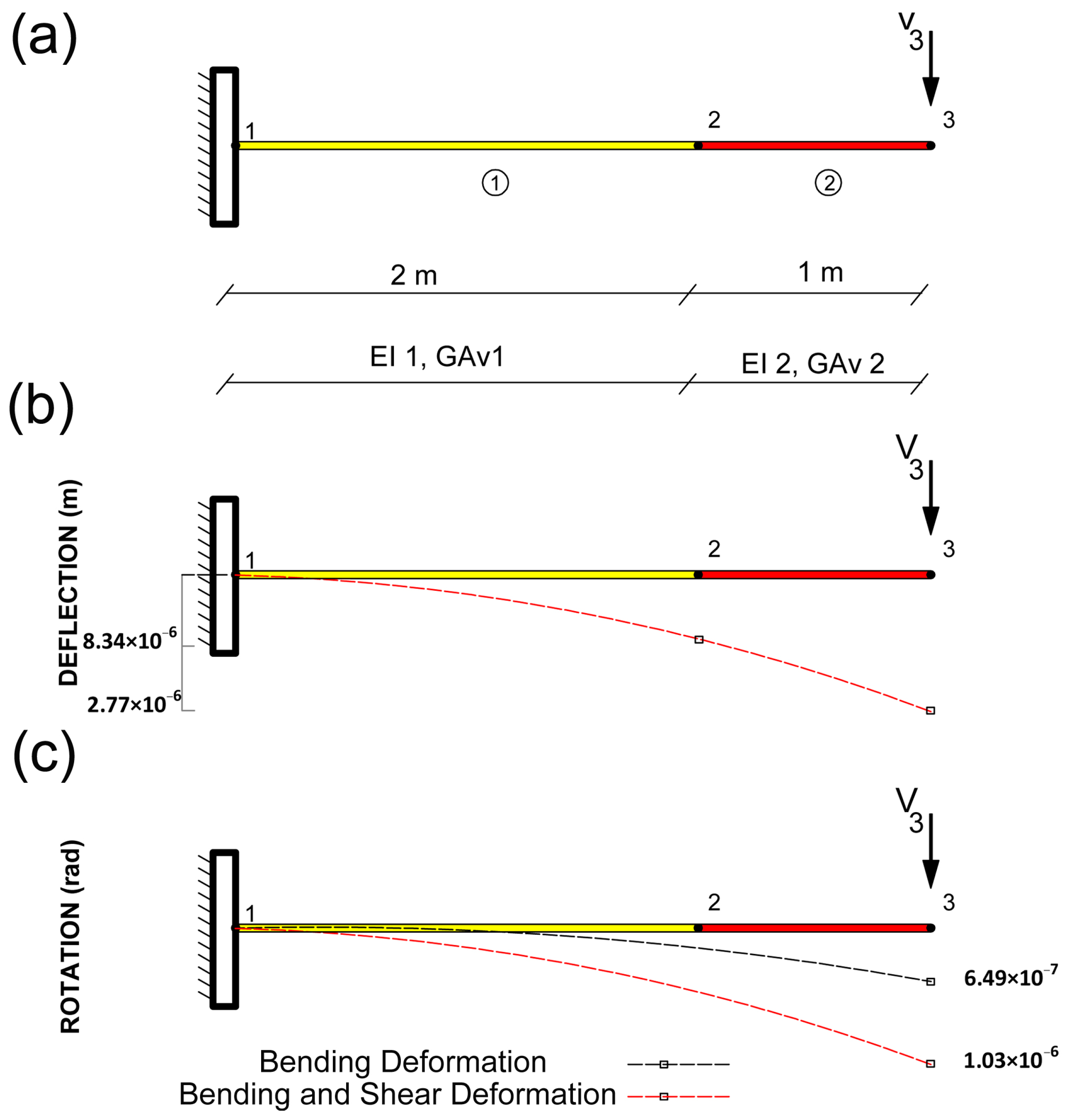
3.2. Example 2: Cantilever Beam with Two-Iteration Processes

Consider a cantilever beam with 3-m length, the same cross-section, and the same properties as in Example 3.1 modeled with one beam element and two nodes as presented in Figure 5. The boundary conditions of the structure are the total horizontal and vertical displacements and rotation due to bending restricted in node 1 (this is to say u₁ = v₁ = w_b1 = 0). The only external force applied is assumed as a concentrated vertical force in node 3 of 100 kN (V₃ = 100 kN). As in the previous example, the length of the elements L, the Poisson’s ratio, and the Young’s modulus E are assumed as known in the inverse analysis, while the inertia I, and the shear area A_v for elements 1 and 2 are assumed as unknown. To obtain these four unknown parameters, the measurement set should include at least four rotations. Nevertheless, the analysis of the traditional OM proves that no set of four rotations in the COM enables the proper identification of the unknown parameters. Therefore, a set of vertical deflection and rotation should be measured together in this example. To perform the COM2, a measurement set that consists of two rotations and two vertical deflections (w₂, w₃ and v₂, v₃) is employed. The rotations and the vertical deformations including the shear effects of this structure are presented in Figure 5.

To check the robustness of the method, a set of random values is chosen for the inertia and shear area to be used to calculate the hypothetical site measurements. A total of 50 different random sets of the initial value coefficients for the inertia and the shear area were randomly chosen between 0.8 and 1.2 of the theoretical values. Also, no matter what set of the initial value is chosen, in all circumstances, the obtained values of the two-iteration process have proper convergence to the real values of the mechanical properties. The normalized average, standard deviation, and coefficient of variation of the remaining results as well as the mode are presented in

Table 3. Obtained results from random initial values of example 2.

Parameter	Average	CoV	Standard Deviation
EI1	1.000	8.783 × 10−7	8.783 × 10−7
EI2	1.000	9.118 × 10−7	9.117 × 10−7
GAv1	1.000	0.000	0.000
GAv2	1.000	0.000	0.000

.

These results prove the adequate convergence of the proposed methodology in cantilever beams for random initial values of the unknown parameters. These results show the applicability of the proposed methodology in cantilever structures. It is important to highlight that the obtained results of the original COM process for this example lack physical meaning, as ratios of 0.562 and 3.000 were obtained for the inertia in I₁ and I₂, respectively.

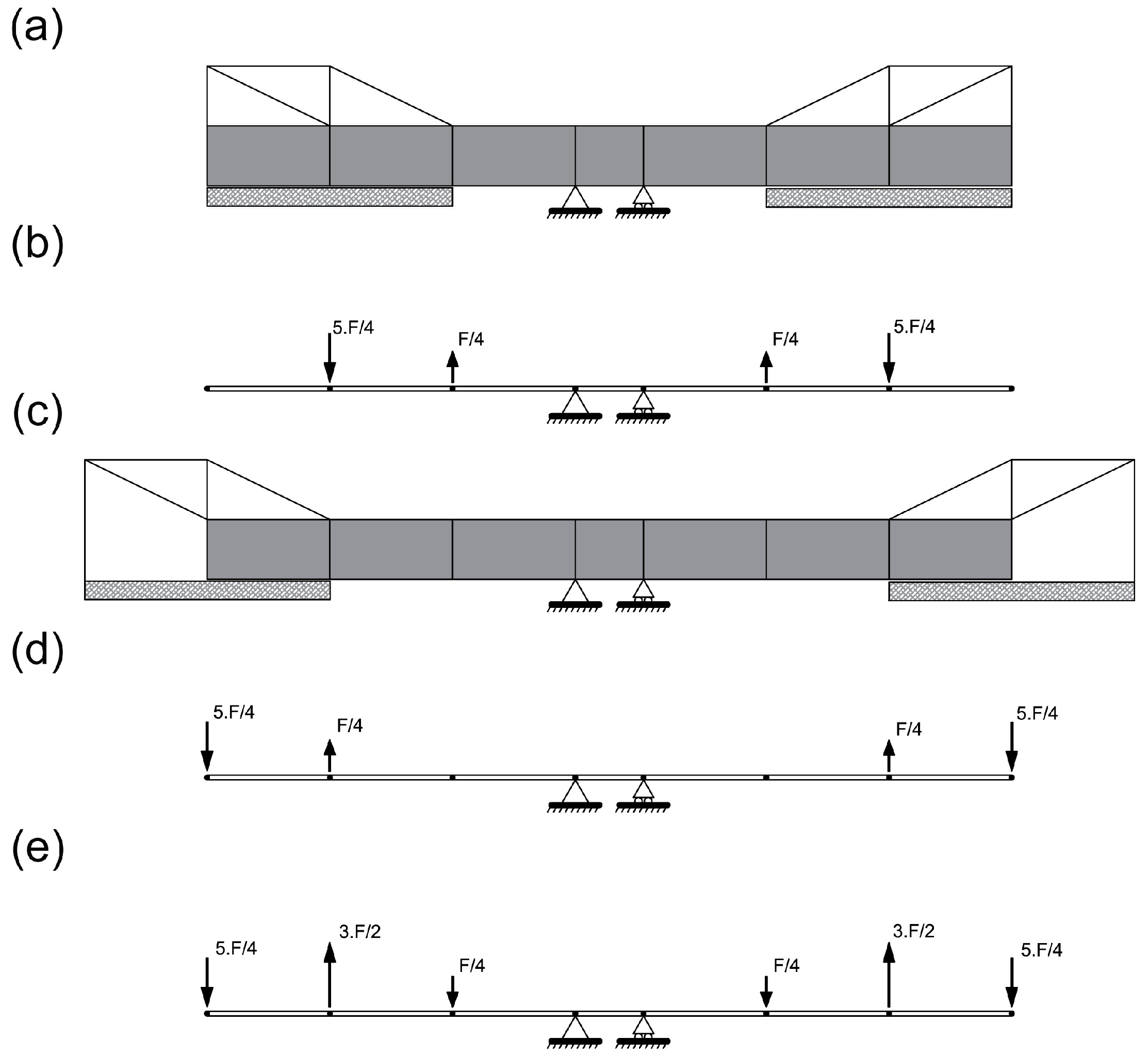
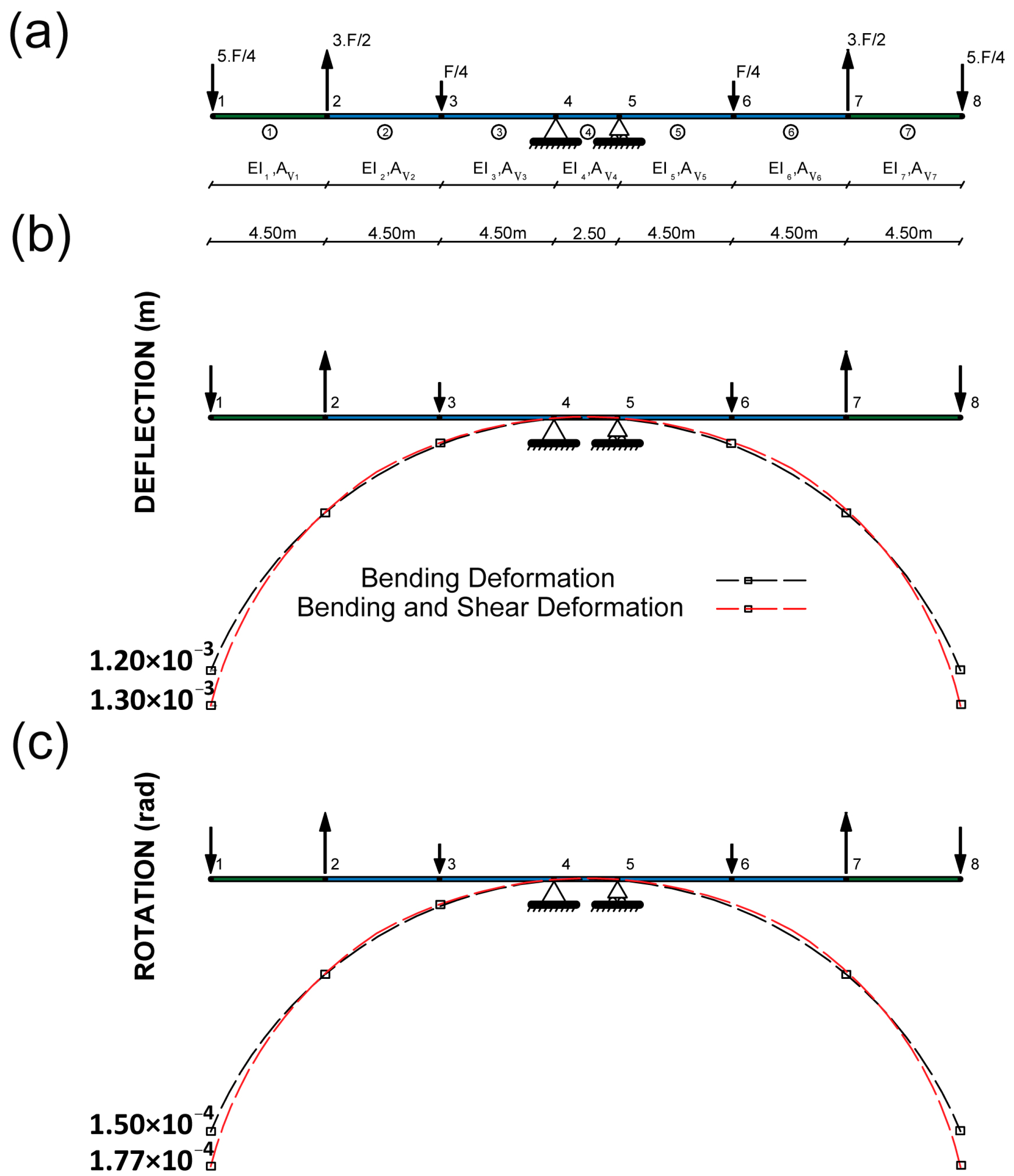
3.3. Example 3: Application to a Simplified Model of a Composite Bridge

To show the application of the proposed methodology to a real structure, the problem of the construction of a bridge by the balanced cantilever method is studied in Section 4.

In these structures, deflections should be anticipated in advance in order to calculate how to build the precamber structures in the different segments. To update this precamber structure for every step during its construction, complete topographic surveying is usually performed. Therefore, an inverse analysis can be employed for providing information for this model updating process. However, shear effects might not play a very important role for a fully developed cantilever; neglecting the effects of the shear rotation in the first segment will lead to the unreliable estimation of the bending stiffness. It is important to highlight that a simplified model of the Yunbao Bridge over the Yellow River in China (see Figure 6) is chosen to demonstrate the feasibility of the proposed methodology. Future research objectives include working with real on-site measurements to enhance the applicability of the method to real structures. Implementing this application will require the creation of more elaborate models. The structure span is 90 m long, but only an intermediate construction stage is considered in this example. The studied construction stage includes the construction of two symmetric cantilevers. The length of each deck segment is 4.5 m and the length of the segment over the pile is 2.5 m. The total length of the model is 29.5 m. The effects of creep and shrinkage in the concrete are overlooked. The connection between the concrete and the steel is assumed as rigid (total connection), and the relative slip between both materials is neglected. Hence, the steel sections of segments contribute very little to the axial and bending stiffness of the composite cross-section. Following Tomás’ assumptions for this structure [10] shear is transferred only by the steel webs. Therefore, the value of the Poisson’s ratio in this example is considered for steel and equal to 0.3. In addition, Young’s modulus is considered 35 GPa. It is important to emphasize that all measurements are generated in numerical form, and the representation of the bridge structure is a simplification. To validate the method’s applicability in monitoring real-world structures, on-site data from actual structures will be analyzed in the future. The mechanical and material properties of Example 3 by the method of the transformed section are listed in

Table 4. Properties of the Finite Element Model of the bridge.

Parameters	Elements 1 and 7	Elements 2 and 6	Elements 3 and 5	Element 4
area [m2]	12.385	12.520	12.670	12.75
shear area [m2]	8.17	9.29	10.62	11.37
inertia [m4]	38.346	48.347	67.98	60.921

[46].

Actual on-site data is not considered in this structure and the structural response is simulated numerically. The load test used simulates the movement of the formwork traveler (Figure 7). The weight F of the formwork traveler (weight of formwork included) is considered 60% of the weight of the segment (1041 kN). The effect of each form traveler in the deck is considered in two vertical forces. The values of these two forces are 0.25F and 1.25F (226 kN upwards and 1267 kN downwards). The load case of the bridge model is calculated by reducing the effects of stage i (Figure 7a), from stage i + 1 (Figure 7c), wherein the formwork traveler is moved forward to the next segment. The load cases of the stages i and i + 1 are expressed in Figure 7b,d, respectively. The consequent load case introduced in the simulation is shown in Figure 8e. It is important to highlight that the vertical resultant of such forces on each side of the cantilever is zero.

The simplified FEM of this structure is presented in Figure 8. This FEM includes seven elements and six concentrated loads. In this example, we exclusively analyzed the flexural and shear responses. Notably, the axial resistance mechanism was omitted since no axial forces were introduced in the applied loading scenario. Consequently, the values of the cross-sectional areas are not observed, given that they have no impact on the inverse analysis. As shear stiffness and bending stiffness from elements 2, 3, 4, 5 and 6 are supposed to be observed from the previous construction steps, such properties are considered as known. Hence, the shear and bending stiffness of the newly built elements (elements 1 and 7) are the targets of the analysis. This is to say I₁, I₇ and A_v1, A_v7 are assumed as unknowns.

In this example, there are four unknowns (it is to say EI₁, GA_v1 and EI₇, GA_v7). In order to identify the four unknown mechanical properties, a set of at least four measurements is required. The analysis of the OM proves that the COM is not able to observe any structural properties by only measuring the rotations in this example. To observe the structural parameters with the proposed methodology, the variation of deflection and rotation should be taken into account (that is to say w₁, v₂ and w₇, v₆). The value of the theoretical rotation and vertical deflection of node 1 are presented in Figure 8b,c. Timoshenko’s beam theory is used to calculate the values of measured variables in node number 1 (the value at node number 7 is the same).

The initial value coefficients of the unknown inertia and shear area (I₁, I₇ and A_v1, A_v7) were randomly chosen between a ratio of 0.8 and 1.2 of the theoretical values. The 50 analyzed random initial values are performed. Also, no matter what set of the initial value is chosen, in all circumstances the obtained values of the two-iteration processes have proper convergence to the real values of the inertia. The normalized average, standard deviation, and coefficient of variation of the remaining results as well as the mode are presented in

Table 5. Obtained results from random initial values of bridge example.

Parameter.	Average	CoV	Standard Deviation
EI1	1.000	8.237 × 10−7	8.237 × 10−7
EI7	1.000	8.903 × 10−7	8.903 × 10−7
GAv1	0.617	0.740	0.456
GAv7	0.256	0.305	0.078

.

These results prove the adequate convergence of the proposed methodology in a bridge structure for the random initial values of the unknown parameters. These results prove the efficiency of the proposed COM to estimate the inertia when the effects of shear rotations are considered, in the case that the shear area cannot be observed by the proposed method. It is to say that the traditional COM is not able to identify the value of the mechanical properties and it lacks physical meaning when the theoretical rotations are measured. In addition, it is important to highlight that, as far as the authors know, no other SSI method based on SMM in the literature is able to include the effects of these rotations in the inverse simulation.

4. Discussion

The applicability of the proposed methodology is illustrated by several academic examples. In addition, to illustrate the applicability of the proposed method on actual structures, a simplified model of an intermediate construction stage of a cantilever composite bridge in China is studied. It is important to highlight that all the measurements are generated numerically and the bridge structure is simplified. The example results clearly demonstrate that when actual rotation measurements on-site are employed in the COM, the COM is not able to properly observe any material properties even in very simple structures such as in examples 1 and 2; the observed values with the COM either lack physical meaning or contain significant errors. Conversely, the 2COM procedure, proposed by the authors in this paper, consistently exhibits its power by accurately capturing the inertia and shear areas (shear and flexural stiffness) in the same scenarios. In the context of the bridge example, the COM method once again falters in observing the shear and flexural stiffness, and its observation lacks physical meaning. However, despite the increased complexity of this example, the 2COM method, while not achieving pinpoint accuracy in observing the shear area, demonstrates a commendable ability to accurately observe the inertia. It is important to highlight that, to the best of the authors’ knowledge, no other SSI method based on SMM in the existing literature is able to include the effects of shear rotations in the inverse simulation. The result shows the robustness and power of the 2COM method when it works with the actual rotation measurement, while other SSI models are not able to observe any properties. Future research aims to transition from numerical simulations to practical implementation with real structures. This transition will involve addressing the challenges associated with acquiring and working with on-site measurements, as well as accounting for potential modeling errors. By doing so, we intend to enhance the applicability and relevance of our method to real-world engineering scenarios. A deeper analysis of the shear and flexural rotations is presented by Emadi et al. [24]. This work also includes a parametric analysis of these deformations for different beam geometries.

5. Conclusions

Structural system identification methods are essential tools for engineers and researchers in assessing and understanding the behavior of complex structures. Among these methods, stiffness matrix methods have long been a cornerstone, providing valuable insights into structural properties. However, it is important to note that the traditional stiffness matrix methods, like many methods in the literature, have their limitations. One significant limitation is the neglect of the shear rotations, which can have a profound impact on the structural response, particularly in the case of deep beams. Ignoring the shear rotations can lead to substantial errors in estimating the structural parameters, potentially jeopardizing the integrity of real-world structures. To fill this gap, the formulation of the constrained observability method is updated to include the effects of the shear rotations. The inclusion of the shear rotations in the constrained observability method framework is a significant advancement, as it addresses a fundamental limitation of the traditional structural system identification methods and improves the accuracy and reliability of structural parameter estimates. This application leads to an iterative process where the initial values of the estimates are successively updated. The applicability of the proposed methodology is illustrated by several academic examples. In addition, to illustrate the applicability of the proposed method on actual structures, a simplified model of an intermediate construction stage of a cantilever composite bridge in China is studied. The results of this study show how the value of structural properties can be observed by 2 COM when the actual rotations are included into the measurement set. This research presents the application of the method for error-free measurement sets. This research represents a significant step forward in structural system identification. Incorporating the shear rotations into the constrained observability method demonstrates how the accuracy of structural parameter estimates can be improved when the shear rotation effects are included into the equations.

References

1. Albero, V.; Espinós, A.; Serra, E.; Romero, M.L.; Hospitaler, A. Numerical study on the flexural behaviour of slim-floor beams with hollow core slabs at elevated temperature. Eng. Struct. 2019, 180, 561–573. [Google Scholar] [CrossRef]
2. Turgut, C.; Jason, L.; Davenne, L. Structural-scale modeling of the active confinement effect in the steel-concrete bond for reinforced concrete structures. Finite Elem. Anal. Des. 2020, 172, 103386. [Google Scholar] [CrossRef]
3. Weaver, W.; Were, J.M. Computer-Oriented Direct Stiffness Method. In Matrix Analysis of Framed Structures; Springer: Boston, MA, USA, 1990. [Google Scholar] [CrossRef]
4. Sadowski, A.J. On the advantages of hybrid beam-shell structural finite element models for the efficient analysis of metal wind turbine support towers. Finite Elem. Anal. Des. 2019, 162, 19–33. [Google Scholar] [CrossRef]
5. Kawano, A.; Zine, A. Reliability evaluation of continuous beam structures using data concerning the displacement of points in a small region. Eng. Struct. 2019, 80, 379–387. [Google Scholar] [CrossRef]
6. Aguirre, A.; Codina, R.; Baiges, J. A variational multiscale stabilized finite element formulation for Reissner–Mindlin plates and Timoshenko beams. Finite Elem. Anal. Des. 2023, 217, 103908. [Google Scholar] [CrossRef]
7. Ozdagli, A.I.; Liu, B.; Moreu, F. Measuring Total Transverse Reference-Free Displacements for Condition Assessment of Timber Railroad Bridges: Experimental Validation. J. Struct. Eng. 2018, 144, 040180471. [Google Scholar] [CrossRef]
8. Liu, S.; D Ziemian, R.; Chen, L.; Chan, S.-L. Bifurcation and large-deflection analyses of thin-walled beam-columns withnon-symmetric open-sections. Thin-Walled Struct. 2018, 132, 287–301. [Google Scholar] [CrossRef]
9. Dahake, A.; Ghugal, Y.; Uttam, B.; Kalwane, U.B. Displacements in Thick Beams using Refined Shear Deformation Theory. In Proceedings of the 3rd International Conference on Recent Trends in Engineering & Technology, Cochin, India, 18 January 2014. [Google Scholar]
10. Tomas, D.; Lozano-Galant, J.A.; Ramos, G.; Turmo, J. Structural system identification of thin web bridges by observability techniques considering shear deformation. Thin-Walled Struct. 2018, 123, 282–293. [Google Scholar] [CrossRef]
11. Dym, C.L.; Williams, H.E. Estimating Fundamental Frequencies of Tall Buildings. J. Struct. Eng. 2007, 133, 1479–1483. [Google Scholar] [CrossRef]
12. Yan, J.; Zhou, B.; Yang, Z.; Xu, L.; Hu, H. Mechanism exploration and effective analysis method of shear effect of helically wound structures. Finite Elem. Anal. Des. 2022, 212, 103840. [Google Scholar] [CrossRef]
13. EN 1992-1-1; Eurocode 2: Design of Concrete Structures—Part 1-1: General Rules and Rules for Buildings. CEN: Brussels, Belgium, 2002.
14. ACI Committee 318. Building Code Requirements for Structural Concrete and Commentary; American Concrete Institute: Detroit, MI, USA, 2000. [Google Scholar]
15. Timoshenko, S.P. On the correction for shear of the differential equation for transverse vibrations of prismatic bars. Philos. Mag. 1921, 41, 742–746. [Google Scholar] [CrossRef]
16. CSI. CSI Analysis Reference Manual for SAP2000, ETABS, SAFE and CSiBridge; Computers and Structure, Inc.: Berkeley, CA, USA, 2016. [Google Scholar]
17. Keo, P.; Nguyen, Q.-H.; Somja, H.; Hjiaj, M. Derivation of the exact stiffness matrix of shear-deformable multi-layered beam element in partial interaction. Finite Elem. Anal. Des. 2016, 112, 40–49. [Google Scholar] [CrossRef]
18. Pisano, A.A. Structural System Identification: Advanced Approaches and Applications. Ph.D. Thesis, Università di Pavia, Pavia, Italy, 1999. [Google Scholar]
19. Zhang, F.; Yang, Y.; Xiong, H.; Yang, J.; Yu, Z. Structural health monitoring of a 250-m super-tall building and operational modal analysis using the fast bayesian FFT method. Struct. Control Health Monit. 2019, 26, e2383. [Google Scholar] [CrossRef]
20. Lu, Y.; Panagiotou, M. Three-Dimensional Cyclic Beam-Truss Model for Nonplanar Reinforced Concrete Walls. J. Struct. Eng. 2014, 140, 04013071. [Google Scholar] [CrossRef]
21. Reddy, J.N. An Introduction to the Finite Element Method; McGraw-Hill Education: New York, NY, USA, 2006; ISBN 9780072466850. [Google Scholar]
22. Pickhaver, J.A. Numerical Modelling of Building Response to Tunneling. Ph.D. Thesis, University of Oxford, Oxford, UK, 2006. [Google Scholar]
23. Przemieniecki, J.S. Theory of Matrix Structural Analysis; Courier Corporation: Chelmsford, MA, USA, 1968; p. 19151. [Google Scholar]
24. Emadi, S.; Ma, H.; Lozano-Galant, J.A.; Turmo, J. Simplified Calculation of Shear Rotations for First-Order Shear Deformation Theory in Deep Bridge Beams. Appl. Sci. 2023, 13, 3362. [Google Scholar] [CrossRef]
25. Sirca, G.F., Jr.; Adeli, H. System identification in structural engineering. Sci. Iran. 2012, 19, 1355–1364. [Google Scholar] [CrossRef]
26. Pereira, R.L.; Lopes, H.N.; Pavanello, R. Topology optimization of acoustic systems with a multiconstrained BESO approach. Finite Elem. Anal. Des. 2022, 201, 103701. [Google Scholar] [CrossRef]
27. Sun, R.; Chen, G.; He, H.; Zhang, B. The impact force identification of composite stiffened panels under material uncertainty. Finite Elem. Anal. Des. 2014, 81, 38–47. [Google Scholar] [CrossRef]
28. Gevers, M. A personal view of the development of system identification: A 30-year journey through an exciting field. IEEE Control Syst. 2006, 26, 93–105. [Google Scholar]
29. Hoang, T.; Foret, G.; Duhamel, D. Dynamical response of a Timoshenko beams on periodical nonlinear supports subjected to moving forces. Eng. Struct. 2018, 176, 673–680. [Google Scholar] [CrossRef]
30. Kim, N. Dynamic stiffness matrix of composite box beams. Steel Compos. Struct. 2009, 9, 473–497. [Google Scholar] [CrossRef]
31. Erdogan, Y.S.; Catbas, F.N.; Bakir, P.G. Structural identification (St-Id) using finite element models for optimum sensor configuration and uncertainty quantification. Finite Elem. Anal. Des. 2014, 81, 1–13. [Google Scholar] [CrossRef]
32. Chatzieleftheriou, S.; Lagaros, N.D. A trajectory method for vibration based damage identification of underdetermined problems. Struct. Control. Health Monit. 2017, 24, e1883. [Google Scholar] [CrossRef]
33. Mai, H.T.; Truong, T.T.; Kang, J.; Mai, D.D.; Lee, J. A robust physics-informed neural network approach for predicting structural instability. Finite Elem. Anal. Des. 2023, 216, 103893. [Google Scholar] [CrossRef]
34. He, Y.; Zhao, Z.-L.; Cai, K.; Kirby, J.; Xiong, Y.; Xie, Y.M. A thinning algorithm based approach to controlling structural complexity in topology optimization. Finite Elem. Anal. Des. 2022, 207, 103779. [Google Scholar] [CrossRef]
35. Catbas, N.; Kijewski-Correa, T.; Aktan, E. Structural Identification of Constructed Systems: Approaches, Methods, and Technologies for Effective Practice of St-Id; American Society of Civil Engineers: Reston, VA, USA, 2013. [Google Scholar] [CrossRef]
36. Dincal, S.; Stubbs, N. Nondestructive damage detection in euler-bernoulli beams using nodal curvatures—Part I: Theory and numerical verification. Struct. Control Health Monit. 2014, 21, 303–316. [Google Scholar] [CrossRef]
37. Wei, G.; Lardeur, P.; Druesne, F. A new solid-beam approach based on first or higher-order beam theories for finite element analysis of thin to thick structures. Finite Elem. Anal. Des. 2022, 200, 103655. [Google Scholar] [CrossRef]
38. Nguyen, N.-T.; Kim, N.-I.; Lee, J. Mixed finite element analysis of nonlocal Euler–Bernoulli nanobeams. Finite Elem. Anal. Des. 2015, 106, 65–72. [Google Scholar] [CrossRef]
39. Leblouda, M.; Junaid, M.T.; Barakat, S.; Maalej, M. Shear buckling and stress distribution in trapezoidal web corrugated steel beams. Thin-Walled Struct. 2017, 113, 13–26. [Google Scholar] [CrossRef]
40. Emadi, S.; Lozano-Galant, J.A.; Turmo, J. Analyzing the Effects of Shear Deformations on the Constrained Observability Method, Bridge Maintenance, Safety, Management, Life-Cycle Sustainability and Innovations; CRC Press: Boca Raton, FL, USA, 2021; pp. 3755–3762. [Google Scholar]
41. Lozano-Galant, J.A.; Nogal, M.; Castillo, E.; Turmo, J. Application of observability techniques to structural system identification. Comput.-Aided Civ. Infrastruct. Eng. 2013, 28, 434–450. [Google Scholar] [CrossRef]
42. Lei, J.; Nogal, M.; Lozano-Galant, J.A.; Xu, D.; Turmo, J. Constrained observability method in static structural system identification. Struct. Control Health Monit. 2017, 25, e2040. [Google Scholar] [CrossRef]
43. Emadi, S.; Lozano-Galant, J.A.; Xia, Y.; Ramos, G.; Turmo, J. Structural system identification including shear deformation of composite bridges from vertical deflections. Steel Compos. Struct. 2019, 32, 731–741. [Google Scholar]
44. Emadi, S. Application of Observability Techniques to Structural System Identification Including Shear Effects. Ph.D. Thesis, Universitat Politècnica de Catalunya-BarcelonaTech, Barcelona, Spain, 2020. [Google Scholar]
45. MATLAB and Optimization Toolbox Release; The MathWorks, Inc.: Natick, MA, USA, 2017.
46. Chen, Y.S.; Yen, B.T. Analysis of Composite Box Girders, March 1980; Fritz Laboratory Reports; Fritz Laboratory: Bethlehem, PA, USA, 1980; Paper 447; Available online: http://preserve.lehigh.edu/engr-civil-environmental-fritz-lab-reports/447 (accessed on 20 July 2023).
47. Dong, X.; Zhao, L.; Xu, Z.; Du, S.; Wang, S.; Wang, X.; Jin, W. Construction of the Yunbao Bridge over the yellow river. In Proceedings of the EASEC-15, Xi’an, China, 11–13 October 2017. [Google Scholar]
Figure 1. (a) A simply supported beam with a zoomed support. (b) Euler–Bernoulli’s beam theory on the beam support. (c) Timoshenko’s beam theory on beam support.
Applsci 13 11456 g001
Figure 2. Flow chart of structural system identification by COM.
Applsci 13 11456 g002
Figure 3. Flowchart of 2COM.
Applsci 13 11456 g003
Figure 4. Example 1. (a) FEM for a simply supported beam. (b) Deformed shape with the value of bending vertical deformation and with bending and shear vertical deformation at Node 2. (c) Deformed shape with bending rotation and with bending and shear rotation at Node 1.
Applsci 13 11456 g004
Figure 5. Example 2. (a) FEM for a cantilever beam. (b) Deformed shape with the value of bending vertical deformation and with bending and shear vertical deformation at node 2. (c) Deformed shape with bending rotation and with bending and shear rotation at node 2.
Applsci 13 11456 g005
Figure 6. Composite bridge on-site [47].
Applsci 13 11456 g006
Figure 7. Definition of the load case: (a,b) Stage i. (c,d) Stage i + 1. (e) Load case used for the inverse analysis.
Applsci 13 11456 g007
Figure 8. Example 3. (a) FEM of the bridge with load case used for inverse analysis. (b) Deformed shape with the value of bending vertical deformation and with bending and shear vertical deformation at node 1. (c) Deformed shape with bending rotation and with bending and shear rotation at node 1.
Applsci 13 11456 g008