Measurement of CO₂ Emissions by the Operation of Freight Transport in Mexican Road Corridors

Abstract

The freight transport industry in Mexico has grown significantly since the establishment of trade agreements in North America, which has brought significant environmental consequences to the main transport corridors. This paper proposes a methodology for the estimation of emissions for freight vehicles on road transportation corridors. The variables included in this analysis allow adequate characterization of the conditions of the vehicle fleet, the geometry and the quality of the road, the environment, and the average annual daily traffic (AADT) of heavy vehicles. The results were structured to show two indicators, the amount of CO₂ emissions per kilometer and the amount of emissions per tonne transported. These results will allow establishing a baseline of CO₂ emissions through which we can implement actions in the road transport sector to reduce greenhouse gases (GHG) to mitigate climate change and develop parameter values for use in Cost Benefit Analysis. The indicators can also be applied to geospatial modeling of emissions in road transport corridors and forecast its growth.

1. Introduction

The challenge in recent years for most countries on environmental issues is achieving global action against climate change. In order to take action, governments have developed a set of targets aimed at reducing emissions of greenhouse gases (GHG) in programs and strategies at the national level, which are documented in several research studies [1,2,3]. At the same time, governments are being prepared to implement adaptation measures to reduce the vulnerability of their critical systems, such as transport [4]. The World Road Association has documented some examples in countries such as England, Scotland, Japan, the USA, Australia, and Germany [5].

Several countries have found that the largest source of GHG generation is transportation. In this sense, the Organization for Economic Co-operation and Development (OECD) highlights that the sector accounted for approximately 13% of overall GHG emissions and 24% of CO₂ emissions from fossil fuel combustion in 2006 [6]. Considering the development path of the transport sector in developed countries, there is little doubt that the road transport sector emissions will be dominant [7]. Nevertheless, a major concern for road freight transport is the fact that energy consumption is growing at a faster rate than energy used by cars and buses [8]. Freight transportation consumes about 43% of all fuel used in transportation and is responsible for a major share of transport-related emissions of nitrogen oxides, unburned hydrocarbons, and fine particulate matter [9].

The freight transport industry in Mexico has grown significantly since the establishment of the North American Free Trade Agreement in 1994 (NAFTA, now USMCA), which has brought significant environmental consequences to the main transport corridors [10]. Commodity movements in North America are concentrated in trade between Canada and the USA, and between Mexico and the USA.

According to the Secretariat of Infrastructure, Communications and Transportation in Mexico (SICT, 2021), around 700 million tonnes of goods were carried by different modes of transport in 2020 (7% less than in 2019 due to the pandemic of COVID-19) [11]. More than 77% of goods are transported by heavy-duty vehicles, which is currently the source generating the highest number of emissions and other environmental impacts such as noise, accidents, solid waste generation [12,13], and climate change [14]. Trucks leading the movement in freight transportation (by value) among the three-country members of the North American Free Trade Agreement (NAFTA), now called the United States–Mexico–Canada Agreement (USMCA) [15]. Worldwide, it is highlighted that there is significant attention on road transport, as this is the dominant mode of freight movement [16,17]. In this sense, the Mexican transport sector is one of the largest sources of GHG contribution, which represents 25% of the national total, with 171 Mt CO₂eq issued in 2015, distributed by roads (159.4 Mt CO₂eq), maritime (2.6 Mt CO₂eq), railroad (2.5 Mt CO₂eq), electric (not significant), and air (6.3 Mt CO₂eq) with information of the Sixth National Communication of Mexico [18].

Most studies to measure the impact of climate change on the transport sector are based on the application of methodologies that have set the Intergovernmental Panel on Climate Change (IPCC) called National Emissions Inventories (developed by 185 countries that are members of Parties Conferences in the United Nations Framework Convention on Climate Change). The methodologies for the inventory of emissions from the transport sector have a top-down approach, converting the energy consumption of the country through emission factors in GHG emissions [19]. Using this approach, some studies have estimated emissions in the transport sector [20,21].

Researchers and technical agencies of various countries have developed inventories with more detailed information, using methodologies with a bottom-up approach [22,23,24]. This type of inventory in the transport sector focuses on ground transportation in cities, but it does not usually include intercity transportation (road transport).

In-depth studies of emission inventories on roads have been identified specifically for freight transport. A study based on surveys applied to transport companies was carried out, where information was gathered about energy consumption, distance traveled, and vehicle performance by Heavy Goods Vehicle (HGV) weight class. The methods of calculation in the UK use four approaches (described in Section 2) to estimate CO₂ emissions from road freight transport. The conclusion of this study describes the need to reconcile differences in truck-km estimates based on surveys and roadside traffic counts depending on the scope of the analysis [16]. Another study evaluates the environmental impact of a major freight corridor in California, particularly associated with heavy-duty diesel trucks. The baseline was developed using a traffic microsimulation tool (TransModeler). In this study, vehicle emissions depend on vehicle type, model year, and fuel type. This methodology estimates instantaneous emissions and the fuel consumption rate for different vehicle types and estimates emissions under various traffic operational scenarios (such as congestion, traffic signals, and High-occupancy vehicle lanes). The results show that utility is applied to this process to evaluate scenarios; however, they exclude infrastructure characteristics [25].

The Commission for Environmental Cooperation developed a study to determine the actual impact of CO₂ emissions in the transport corridors of North America and its future impact [10]. The methodology developed a bottom-up approach; however, a few variables such as traffic flow, emission rates, corridor data, and truck data were considered in the analysis in order to establish comparability between the three countries of the region (Canada, Mexico, and the United States of America). The information used in this study also does not include detailed information about road characteristics to obtain a reliable measure of emissions to construct a baseline.

To implement emission reduction strategies, it is necessary to have a reliable emission inventory that allows the establishment of a baseline in order to measure the impact of the action on the mitigation of climate change. In order to reduce GHG emissions in freight transportation, it requires using appropriate emission models and integrating data into the bottom-up methodology in the planning process, to develop a reliable emission inventory [26].

Rapid urbanization and economic growth in developing countries have spurred air pollution, especially in the road transport sector. The increasing demand for petroleum-based fuels and their combustion in internal combustion (IC) engines have adverse effects on air quality, human health, and global warming [27]. Addressing climate change in developing countries poses a fundamentally different challenge. Developing countries will continue to increase their emissions due to economic growth and a better quality of life [28].

Forecasts of emission in Mexico trends shown in Figure 1 show a significant growth in GHG emissions [29]. Appropriate strategies are required to reduce these future increases, such as the ones analyzed [30], where 21 GHG mitigation measures were applied to reduce transport sector GHG emissions in Mexico. This, therefore, results in the need to develop a methodology to estimate emissions in transport corridors in developing countries such as Mexico through a bottom-up approach.

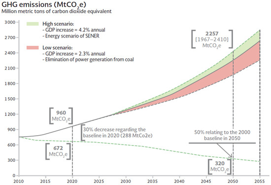
Figure 1. Baseline and objective trajectory of GHG emissions in Mexico 2010–2050. Source: SEMARNAT, 2013. Notes: Gross Domestic Product (GDP); Ministry of Energy (SENER).

The aim of this study, on one hand, is to develop a methodology with a bottom-up approach, with as many variables of road transportation, and to obtain an emission inventory for measuring CO₂ emissions of freight transport in road corridors for Mexico. Additionally, this study seeks to establish environmental indicators with the results applicable to CO₂ in transport corridors.

2. Review of Literature

It is noted that bottom-up methodologies are supported using models for estimating emissions, which are based on various factors that influence energy consumption. A review of several studies to compile various factors that influence energy consumption and emissions generation during freight transport was conducted. The factors were classified into five categories: vehicle (vehicle curb weight, vehicle shape, engine size/type, engine temperature, transmission, fuel type/composition, age, maintenance, and accessories); environment (roadway gradient, pavement type, ambient temperature, altitude, wind conditions, humidity, and surface conditions); traffic (speed, acceleration/deceleration, and congestion); driver (driver aggressiveness, gear selection, and idle time) and operation (fleet size an mix, payload, empty kilometers, and number of stops) [31].

Under the MEET project “Methodologies for estimating air pollutant emissions from transport”, emissions from road transport are calculated with the emission factor and the activity (distance traveled per time unit). Emission factors were estimated through driving cycles by the Transportation Research Laboratory in the UK, particularly for heavy-duty vehicles, and include variables such as road gradient, speed, weight vehicle, and empty vehicles [32].

Four approaches have been adopted in the UK to estimate CO₂ emissions from road freight transport. Approach one employs survey data from the Continuing Survey of Road Goods Transport (CSRGT), using the average efficiency and average annual distance traveled to obtain a measure of total fuel consumption. Approach two utilizes a combination of traffic flow estimates of truck-km with survey-based fuel efficiency estimates. Approach three is similar to approach two, where only the efficiency estimates are based on vehicle test cycles. Approach four estimates of total fuel sales to HGV, which are multiplied by a CO₂ conversion ratio similar to IPPC methodologies [16]. Emission inventories based on IPCC methodologies involve the multiplication of energy consumption by an emission factor according to the activity.

In Colombia, to estimate emissions by trucks, the Handbook Emission Factors for Road Transport (HBEFA) was used [33]. To accomplish this, information on each vehicle was collected, including model, year, type of fuel used, Euro standard, and engine power trucks. The commercial vehicles were equipped with a Global Positioning System (GPS) to obtain second-to-second speed, location, acceleration, and deceleration; the rest of the data were provided by the vehicles’ owners.

It was identified that some emissions models are integrated into a computer program and include different factors to estimate emissions, described as the most relevant to the transport sector. MOBILE6 Vehicle Emission Modeling Software is an emission factor model for predicting gram-per-mile emissions developed by the Environmental Protection Agency [34]. The next emission model developed by EPA is the “Motor Vehicle Emission Simulator (MOVES)”, which is a state-of-the-science emission modeling system that estimates emissions for mobile sources at the national, county, and project level for criteria air pollutants, GHG, and air toxins [35]. Both models have a useful application for estimating emissions from transportation in cities but are more complicated to use for estimating emissions on roads.

The Highway Development and Management System is a decision tool to help with road investment choices (HDM-4). One part of the model allows estimating the social and environmental effects of investment through the sub-model of energy and environmental effects that permit estimating some type of emissions such as CO₂ [36]. Another model used in Europe is the COPERT 4 (Computer Program to Calculate Emission from Road Traffic), which is software to estimate air pollutant emissions from road transport. The development of COPERT 4 has been financed by the European Environment Agency [37]. The COPERT 4 methodology has been developed for the compilation of national inventories or specific studies such as the one developed to assess the sector’s contribution to the total national emissions budget (inventory) of the different fuels [38].

Using a greater number of variables allows a more reliable estimation of emissions, but this must be consistent with the country’s ability to provide information. EPA models (MOBILE6 and MOVES) are widely used in Mexico cities; however, the information for roads is not easy to complete. While the COPERT 4 model can be used, emission factors are more commensurate with the European context. The HDM-4 model was made for roads, and variables for estimating emissions are available in Mexico and are detailed below.

3. Methodology and Data Collection

The framework for estimating emissions from freight transport is mainly defined by the infrastructure (transport corridors), traffic data (annual average daily traffic, vehicle age, and percentage of vehicles loaded), light and heavy vehicles, geography and environmental characterization, and design infrastructure (road design and surface pavement conditions).

3.1. Transport Corridors

A corridor is a broad geographic area, defined by logical, existing, and forecasted travel patterns served by various modal transportation systems that provide important connections within and between regions of the State for people, goods, and services [39]. Travel within the corridor may include vehicle, rail, transit, water, air, or non-motorized means. In the same sense, a transport corridor is the area of origin and destination of traffic flows [40].

In Mexico, transport corridors are defined by the largest movement of freight and passengers across the road network. The first transport corridors were defined through origin–destination data and cargo transported [41]. Transport corridors are placed into a hierarchy using land use models, incorporating the economic value of the freight transported. The results can then be applied to the first strategic planning for the expansion of the corridors in the country. Nowadays, the network is composed of 16 large road corridors that connect the main ports and border crossings, in addition to providing accessibility to major cities that make up the country and Mexico City. Figure 2 shows the main transport corridors in Mexico.

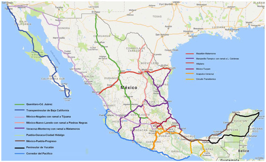
Figure 2. Transport road corridors in Mexico. Source: Own elaboration using Google Maps.

3.2. Traffic Data

The traffic data required are the average annual daily traffic (AADT) of each route in the different sections along its entire length. In Mexico, the SICT has installed and operates a system of traffic measuring, which keeps macroscopic traffic variables updated annually, such as volumes and speed information. Traffic data also allows vehicle classification (Table 1), according to the percentages extracted from the highway traffic data of the SICT [42].

Table 1. Vehicle Classification.

FHWA Classification [43] a	Type of Vehicle	SICT Classification [42] b
Class 2 and 3	Light Vehicle	A
Class 4	Bus	B
Class 5	Medium truck (2 axes)	C2
Class 6	Heavy truck (3 axes)	C3
Class 9	Articulated truck (5 axes)	T3-S2
Class 10	Articulated truck (6 axes)	T3-S3
Class 13	Double articulated truck (9 axes)	T3-S2-R4

Source: ^a Data from FHWA (2014) [43] and ^b from the SICT (2020) [42].

The vehicle fleet data provide detailed information for calculating and estimating speeds, operating costs, travel time, and other aspects. It is necessary to also identify the number of passengers, number of wheels and axles, annual kilometers, average vehicle life, working hours and weight, and other data.

The characterization was carried out according to the studies of the Origin and Destination Survey (ODs) that apply the SICT to the country’s roads, which also includes the weights and dimensions of vehicles and the age of the vehicles traveling on the roads. Since the stations for the implementation of the surveys are located at different points every year, it is not possible to apply for a single study. Therefore, the present work decided to use the last results of the monitoring station located on each transport corridor [44]. A summary of the studies to determine the age of the vehicle fleet is shown in Table 2.

Table 2. Average age of the vehicle fleet.

ID Station	Name	Road Section	Year	Transport Corridor	Average Age/Type of Vehicle
					B	C2	C3	T3S2	T3S3	T3S2R4
274	El Cerrito	Querétaro-San Luis Potosí	2011	1	6.5	8.1	13.1	8.1	9.2	6.1
257	Samalayuca III	El Sueco-Ciudad Juárez	2010	2	8.1	7.6	13.1	10	11.9	7.6
249	Las Viguitas	Hermosillo-Nogales	2010	3*	6.3	8.1	14.7	13.1	13.4	8.7
259	El Valiente	Ciudad Obregón-Hermosillo	2010	3*	7	8.4	12.7	10.2	12.2	6.9
229	PC Cuyutlán	Armería-Manzanillo	2009	4	6.9	7.7	9.3	7.3	6.4	4.8
154	Canal SARH	Córdoba-Veracruz (cuota)	2002	5	7.3	10.1	8.6	8.6	4.9	5.6
279	Vega de Alatorre	Poza Rica-Veracruz	2011	6	6.8	9.4	16.4	9.3	9.3	3.6
271	Los Tamarindos	Coatzacoalcos-Salina Cruz	2011	7	10.7	11.1	12.7	12.1	11	6.9
264	Tabasquillo	Villa Hermosa-Cd. Carmen	2010	8	6.4	7.5	9.7	8.3	8.9	6
283	Bacalar	Reforma Agraria-Puerto Juárez	2011	9	9	9	13.2	10.3	14.4	6.5
228	San Felipe	Playa Azul-Manzanillo	2009	10	10	10.3	18.4	11	12.4	14.3
205	La Rosa	Saltillo-Torreón	2006	11	8.3	8.3	12.1	10.1	10.5	8.7
245	Popotla	Tijuana-Ensenada	2010	12	14.5	12.5	13	16.3	15	8.1
237	Cuapiaxtla	Amozoc-Perote	2009	13	8.5	10.5	15.6	8.3	10.8	5.6
292	Palo Blanco	Cuernavaca-Acapulco	2012	14	6.5	8.7	12.9	9.2	9.1	6.2
292	Palo Blanco	Cuernavaca-Acapulco	2011	15	6.5	8.7	12.9	9.2	9.1	6.2
268	Zacatal	Coatzacoalcos-Salina Cruz	2011	16	10.6	10.09	17.7	13.4	15	7.1

Source: Own elaboration based on Mexican Institute of Transportation (2002, 2009, 2010, 2011) [44].

3.3. Geography and Environmental Characterization

In order to use the model, climatological data are acquired, such as precipitation, humidity, temperature, and their average ranges of variation. Köppen climate classification adapted was used to characterize the environmental regions in the country [45]. This scale consists of a worldwide climatic classification that identifies each type of climate with a series of letters, indicating the behavior of temperature and rainfall that characterize this type of climate. Additionally, the transport corridors of the study identified eight climate types (Table 3).

Table 3. Climate classification in México.

No.	Climate Zone	Description
1	Af	Tropical with year-round rainfall
2	Am	Tropical with monsoon rains (short dry)
3	Aw	Tropical with summer rains (winter dry)
4	Bs	Semi-arid (steppe climate)
5	Bw	Arid (desert climate)
6	Cf	Temperate with year-round rainfall
7	Cw	Temperate with summer rain (dry winter)
8	Cs	Temperate with winter rains (dry summers)

Source: Own elaboration based on García (1998) [45].

3.4. Design Infrastructure

The road geometry is related to the angular changes of the vertical and horizontal alignment (curves of the road) and is closely related to the topography. This information was obtained from the road design databases provided by the Secretariat of Infrastructure, Communications and Transportation [46].

The required data on the vertical geometry for the model are elevation (in meters) above mean sea level, for each section, as well as the corresponding vertical slopes in this case per kilometer, which are entered as a percentage, in proportion with the angle of the slope and to the horizontal, the starting point to the end point of the section.

The status indicator that assesses the roads, in terms of the quality of the surface layer for the bearing of vehicles, is the International Roughness Index (IRI). The IRI was developed by the World Bank in the 1980s [47]. The IRI is used to define a characteristic of the longitudinal profile of a traveled wheel track and constitutes a standardized roughness measurement. The commonly recommended units are meters per kilometer (m/km) or millimeters per meter (mm/m). The correlation between the IRI, speed, and vehicle operating costs is one of the most important premises on which the analysis methodology is based, using HDM-4 [36]; parameters that are directly related to fuel consumption, by which the model predicts an approximate of the amount of emissions generated by vehicles.

Surface roughness information is obtained through field inspections conducted with different pieces of equipment across the federal road network of the country (freeways and tollways). The IRIs used for each road section and each corridor are averaged to obtain homogeneous sections, according to the sections of road that were defined mainly by the AADT.

4. Methodological Procedure to Estimate Emissions in Road Transport Corridors

The methodology uses the Social and Environmental Effects (SEA) sub-model of the Highway Development and Management System, known as HDM-4 [36]. The HDM-4 is useful because this tool was specifically designed for roads, and the main objective of this research work is to estimate emissions from road transport in major freight corridors of the country.

The sub-model SEA of HDM-4 calculates at a macro level, the quantity of emissions in the form of chemicals and noise generated by the operation of transport on a road network or road segment, and the energy balance of the life cycle of conservation strategies (see Figure 3).

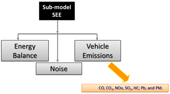
Figure 3. Structure of sub-model of Environmental Effects HDM-4. Source: Own elaboration based on World Road Association (PIARC) [36].

The HDM-4 emission model is based on the proposal by Hammarstrom [48] and predicts emissions from vehicle exhaust in terms of fuel consumption and average speed. Relationships and model coefficients were adjusted in terms of grams per kilometer [49].

Vehicle emission inventory based on a bottom-up approach requires the following information: emission factors according to the number of vehicles, vehicle age, and type of vehicle; the distances traveled by each type of vehicle; environmental data to characterize the study area, such as altitude and temperature; the quality state of the road network and comprising elements such as the pavement surface, operating speeds [32].

The proposed methodology for estimating emissions for transport operations on roads consists of three stages, as shown in Figure 4. The main effort is focused on the first stage, which is necessary to collect traffic data from the transport corridors, as well as obtaining information about the road geometry (horizontal and vertical alignment), characterization of the vehicle fleet (classification, age, etc.), environmental data (altitude, climate zone, etc.), where each road section is located, and the quality of pavement surface thought the IRI (see Section 3 “Methodology and Data Collection”). Stage 2 consists of the data capture process within the HDM-4 to perform all analyses. In Stage 3, the output of the analysis derived from the emissions model is obtained. The following pollutant emissions are estimated: hydrocarbons, nitrogen oxides, sulfur oxides, carbon monoxide, carbon dioxide, and particulate matter [50].

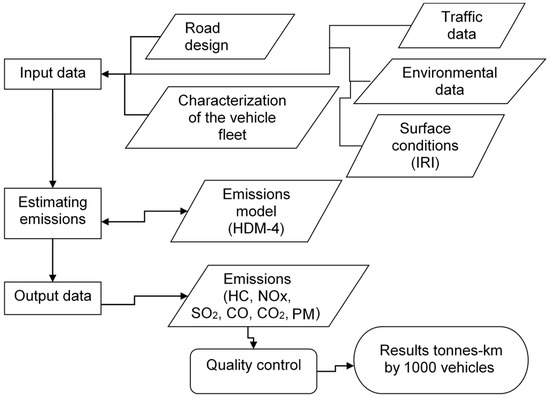
Figure 4. Methodology for estimating emissions of motor vehicles on road corridors. Source: Own elaboration. Notes: hydrocarbons (HC), nitrogen oxides (NOx), sulfur oxides (SO₂), carbon monoxide (CO), carbon dioxide (CO₂) and particulate matter (PM). The results are expressed in tons per kilometer per thousand vehicles.

5. Inventory of Emissions in Road Transport Corridors

In the emission inventory, the daily number of gases emitted into the atmosphere by the operation of transport vehicles through the transport corridors studied has been estimated by 2019. For this analysis, the most complete AADT road data were used.

Each transport corridor was divided into routes (homogeneous road sections and sections according to the surface condition of the road) to simplify the analyses and interpretation of results.

As the first part of an emission inventory, an analysis was developed of all transport corridors, which includes six pollutants quantification of all vehicles passing daily on different roads that integrate the corridors analyzed (hydrocarbons, nitrogen oxides, sulfur oxides, carbon monoxide, carbon dioxide, and suspended particulates).

From the result of the total emissions emitted, it was necessary to extract only those emissions that were generated by vehicles for freight transport. Vehicles used for goods and that circulate mostly on roads in Mexico are shown in Table 1. These vehicles are representative of the emission inventory for freight or goods vehicles. The total CO₂ emissions of each transport corridor for freight transport are shown in Table 4.

Table 4. Tonnes of CO₂ emitted daily by the corridor.

Number	ID Mexican Corridor	Length of Corridor (Kilometers)	CO2 Emissions (Tonnes)
1	México-Nuevo Laredo	1155.61	17,897.68
1.1	Ramal a Piedras negras	316.41	961.82
2	México-Cd Juárez	2003.14	13,687.80
3	México-Nogales	2437.46	10,850.56
3.1	Ramal a Tijuana	761.13	1770.27
4	Manzanillo–Tampico	1364.27	6804.20
4.1	Ramal a Lázaro Cárdenas	609.69	2733.26
5	México-Veracruz	389.16	6224.61
6	Veracruz-Monterrey con ramal a Matamoros	1291.32	3920.84
7	Puebla-Oaxaca-Cd. Hidalgo	1095.14	2289.78
8	México-Puebla-Progreso	1302.35	8482.65
9	Peninsular de Yucatán	1203.24	2068.97
10	Corredor del Pacífico	2045.48	1668.17
11	Mazatlán-Matamoros	1348.29	5376.85
12	Transpeninsular de Baja California	1878.61	1727.22
13	Altiplano	587.15	4524.24
14	Acapulco-Tuxpan	1022.84	3345.52
15	Acapulco-Veracruz	766.81	3715.08
16	Circuito Transístmico	799.57	1467.88

Source: Own elaboration.

The indicators of emissions include only CO₂ emissions generated by freight vehicles, in order to model an environmental indicator in terms of the length of each corridor.

6. Environmental Indicators for Road Transport Corridors

The purpose of an environmental indicator is to identify the size of the effect according to both the descriptive effect to characterize and the estimation of the magnitude in absolute terms. To understand an indicator, this is something that provides a clue to a matter of larger significance or makes perceptible a trend or phenomenon [51].

There are different types of indicators for this study. The environmental impact indicators were developed according to the PSR model (Pressure-State-Response). The pressure indicator describes developments in the release of substances (emissions), physical and biological agents, the use of resources, and the use of land [52,53].

Then, in this study, the indicator to be used will be one of the pressures, which expresses the amount of emissions emitted into the atmosphere by the operation of freight vehicles in the transportation corridors.

The emission indicators were based only on CO₂ emissions generated by freight transport in order to model an environmental indicator considering the length of each corridor. The total emissions of each corridor were determined. Those from freight vehicles were extracted, and the effective lengths of each corridor were measured. The emissions are measured daily, as the AADT is used, but it is also possible to obtain the total annual emissions, multiplying daily emissions by 365. Table 5 shows the parameters for the environmental indicator used.

Table 5. Indicator 1, CO₂ emissions per kilometer for freight vehicles.

Characteristic	Description
Indicator:	CO2 emissions per kilometer
Period:	Annual/Daily
Unit:	Tonnes/Kilometer
What it measure?	The quantity of CO2 emissions per kilometer of freight vehicles.
Type of Indicator:	Pressure

Indicator 1 for each corridor is expressed in the Equation (1):

$$E_{{CO}_2}=\frac{\sum {CO}_{2}emissions of each corridor}{effective length of each corridor}$$

(1)

The amount of CO₂ generated is expressed in tonnes, the effective length of the corridor is expressed in kilometers, and the direct result ($E_{{CO}_2}$) is expressed in tonnes per day of CO₂ per kilometer. Table 6 shows the results of indicator 1 for each road transport corridor.

Table 6. Indicator 1: Tonnes of CO₂ per kilometer by corridor.

Number	ID Mexican Corridor	Length of Corridor (Kilometers)	CO2 Emissions (Tonnes)	Indicator 1 “Tonnes of CO2 per Kilometer”
1	México City-Nuevo Laredo	1155.61	17,897.68	15.49
1.1	Ramal a Piedras negras	316.41	961.82	3.04
2	México City-Cd Juárez	2003.14	13,687.80	6.83
3	México City-Nogales	2437.46	10,850.56	4.45
3.1	Ramal a Tijuana	761.13	1770.27	2.33
4	Manzanillo–Tampico	1364.27	6804.20	4.99
4.1	Ramal a Lázaro Cárdenas	609.69	2733.26	4.48
5	México City-Veracruz	389.16	6224.61	15.99
6	Veracruz-Monterrey con ramal a Matamoros	1291.32	3920.84	3.04
7	Puebla-Oaxaca-Cd. Hidalgo	1095.14	2289.78	2.09
8	México City-Puebla-Progreso	1302.35	8482.65	6.51
9	Peninsular de Yucatán	1203.24	2068.97	1.72
10	Corredor del Pacífico	2045.48	1668.17	0.82
11	Mazatlán-Matamoros	1348.29	5376.85	3.99
12	Transpeninsular de Baja California	1878.61	1727.22	0.92
13	Altiplano	587.15	4524.24	7.71
14	Acapulco-Tuxpan	1022.84	3345.52	3.27
15	Acapulco-Veracruz	766.81	3715.08	4.84
16	Circuito Transístmico	799.57	1467.88	1.84
Average				3.51

According to the results obtained, the Mexico City-Nuevo Laredo corridor is the main generator of CO₂ emissions per kilometer, mainly because it is the corridor with the most cargo traffic in the country connecting the USA and Canada.

To determine this indicator to estimate CO₂ emissions generated by freight vehicles according to the number of tonnes transported per kilometer, additional information is required from the Origin-Destination Survey, effective cargo moving on the road corridor.

Emissions per kilometer were determined with indicator 1. The total weight is determined by information on the gross weight of the loaded and empty vehicles, the percentage of vehicles loaded and empty, and the weight of the average load of vehicles loaded, using Equation (2).

$$Weight of load=\frac{Weight of the average load \ast Percentage of vehicles loaded}{100}$$

(2)

Once the weight of the load has been determined, daily tonnes transported can be estimated by Equation (3).

$$Weight daily tons={AADT}_{Heavy vehicles}\ast {Weight}_{load}$$

(3)

Finally, indicator 2 ($T_{{CO}_2\ast Ton-km}$) is expressed as indicate in Equation (4)

$$T_{CO2\ast Ton-km}=\frac{Emissions tons of {CO}_2\ast 1\ast {10}^6}{Length of corridors\ast Weight daily tons}$$

(4)

Table 7 details the characteristics of indicator 2.

Table 7. Indicator 2: Tonnes of CO₂ per million tonne-kilometers.

Characteristic	Description
Indicator:	Tonnes of CO2 per million tonne-kilometer for freight transport
Period:	Daily
Unit:	Tonnes
What it measure?	The quantity of CO2 emissions on average by freight vehicles on federal highways of Mexico per million tonnes transported per kilometer
Type of Indicator:	Pressure
Geographic coverage:	National

The results of the calculation of indicator 2 “Tonnes of CO₂ per million tonne-kilometer” for each road transport corridor analyzed are shown in Table 8. For this analysis, the length of corridors considers both directions, which may vary when the road has two separate sections.

Table 8. Indicator 2: Tonnes of CO₂ per million Tonnes-kilometer.

Number	ID Mexican Corridor	Length of Corridor Analyzed (Kilometers)	CO2 Emissions (Tonnes)	Weight Daily (Tonnes)	Indicator 2 “Tonnes of CO2 per million tonne-kilometers”
1	México City-Nuevo Laredo	2279.02	17,897.68	64,993	120.83
1.1	Ramal a Piedras negras	543.12	961.82	19,320	91.66
2	México City-Cd Juárez	3656.52	13,687.80	26,912	139.10
3	México City-Nogales	4484.07	10,850.56	20,037	120.77
3.1	Ramal a Tijuana	1057.24	1770.27	16,001	104.65
4	Manzanillo–Tampico	2050.25	6804.20	61,085	54.33
4.1	Ramal a Lázaro Cárdenas	836.29	2733.26	31,478	103.83
5	México City-Veracruz	778.32	6224.61	47,055	169.96
6	Veracruz-Monterrey con ramal a Matamoros	1758.48	3920.84	22,400	99.54
7	Puebla-Oaxaca-Cd. Hidalgo	1581.65	2289.78	7231	200.21
8	México City-Puebla-Progreso	2408.43	8482.65	18,831	187.04
9	Peninsular de Yucatán	1757.18	2068.97	9966	118.15
10	Corredor del Pacífico	2387.46	1668.17	5213	134.03
11	Mazatlán-Matamoros	2423.63	5376.85	7205	307.91
12	Transpeninsular de Baja California	2296.0	1727.22	7571	99.36
13	Altiplano	1109.2	4524.24	15,604	261.40
14	Acapulco-Tuxpan	1833.13	3345.52	15,343	118.95
15	Acapulco-Veracruz	1453.51	3715.08	15,419	165.77
16	Circuito Transístmico	953.25	1467.88	11,218	137.27
Average					143.93

7. Modeling Baseline CO₂ Emissions

The modeling of the baseline through Geographic Information Systems (GIS) was based on the main corridors. These maps allow visualization of where the highest concentration of CO₂ emissions per kilometer of freight transported exists. Figure 5 shows the model based on Google Maps, such as the annual emissions per kilometer (environmental indicator 1).

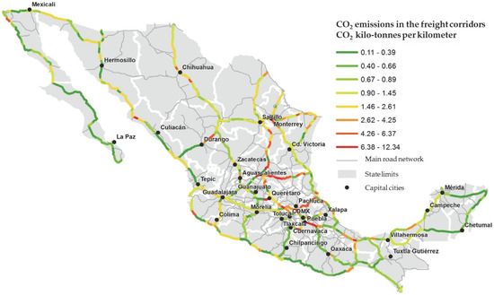
Figure 5. Modeling of CO₂ emissions in the freight corridors. Source: Own elaboration using Google Maps.

Based on the results obtained in the indicators and using the historical growth of heavy vehicles in the corridors, a trend line for freight transportation in Mexico can be constructed [54]. However, the prediction of a trend may not be fully accurate depending on the model used for forecasting [55].

To estimate the growth rate in the freight transportation sector, the growth of the vehicle fleet and cargo transported (including the contraction due to the COVID-19 pandemic) was used, and from the period 2013 to 2020, we obtained a growth of 3.53%, which can be applied to forecasting the growth of emissions over the 2020 baseline estimate of 36.32 Megatonnes of CO₂ (99,517.4 tonnes daily). Figure 6 shows the growth of baseline CO₂ emissions in freight transportation in the main road corridors in Mexico.

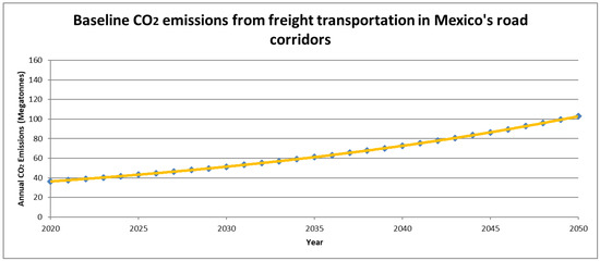
Figure 6. Baseline CO₂ emissions from freight transportation in Mexico’s road corridors. Source: Own elaboration.

8. Conclusions

The proposed methodology has the advantage that it considers in a very detailed way the geometric characteristics of the road, which have an important influence on fuel consumption and emissions generation.

The HDM-4 model was very useful for estimating emissions, as it is developed specifically for roads, and the information required allows for a bottom-up analysis according to the methodologies that are used worldwide to estimate emissions at a higher level of reliability.

The results of CO₂ emissions allow the ability to propose the construction of two environmental indicators of pressure on transport corridors: (i) Tonnes of CO₂ per kilometer by corridor, and (ii) Tonnes of CO₂ per million tonnes-kilometer. The first indicator reflects the number of daily emissions in tonnes emitted into the atmosphere per kilometer of freight in the corridors analyzed, whilst the second represents CO₂ emissions per tonne per kilometer of goods transported in transport corridors analyzed.

These indicators make it possible to establish a diagnosis of freight transportation emissions in Mexico and build a baseline, through which mitigation strategies to reduce GHG emissions can be proposed. This allows the generation of public and private policies to respond to climate change.

The study shows that for Mexico, there is a growth trend in CO₂ emissions produced by road transportation. The results will establish appropriate scenarios to understand the behavior of emissions from freight transport in Mexico and its impact on climate change.

Although the methodology requires multiple data for its analysis, these data are easy to obtain by road organizations; hence, the replication of this study will be very easy for other countries.

The following phases of this research will be used to develop guidelines for decision-makers in the transport sector to help them choose between well-documented strategies to mitigate GHG emissions in the road sector as action against climate change and for optimal use of monetary resources.

With this information, future scenarios can be constructed based on changes in model variables, such as an increase in the AADT or road deterioration through the IRI.

To mitigate climate change, it is important to implement strategies to decarbonize transportation. Using e-fuels, hybrid electric vehicles and electrification (vehicles and infrastructure) could have potential benefits to reduce emissions in road transport corridors in Mexico. Moreover, for sustainability, it is important to consider environmental considerations in freight transportation.

References

- Bodansky, D. Climate commitments: Assessing the options. In Beyond Kyoto: Advancing the International Effort against Climate Change; Pew Center on Global Climate Change (Center for Climate and Energy Solutions): Arlington, TX, USA, 2003. [Google Scholar]
- Chapman, L. Transport and climate change: A review. J. Transp. Geogr. 2007, 15, 354–367. [Google Scholar] [CrossRef]
- Marsden, G.; Rye, T. The governance of transport and climate change. J. Transp. Geogr. 2010, 18, 669–678. [Google Scholar] [CrossRef]
- Intergovernmental Panel on Climate Change (IPCC). Climate Change 2014: Impacts, Adaptation, and Vulnerability. Part A: Global and Sectoral Aspects. Contribution of Working Group II to the Fifth Assessment Report of the Intergovernmental Panel on Climate Change; Field, C.B., Barros, V.R., Dokken, D.J., Mach, K.J., Mastrandrea, M.D., Bilir, T.E., Chatterjee, M., Ebi, K.L., Estrada, Y.O., Genova, R.C., et al., Eds.; Cambridge University Press: Cambridge, UK; New York, NY, USA, 2014. [Google Scholar]
- World Road Association (PIARC). Transport Strategies for Climate Change Mitigation and Adaptation; World Road Association (PIARC): Paris, France, 2016; ISBN 978-2-84060-420-4. [Google Scholar]
- Organization for Economic Co-Operation and Development-International Transport Forum (OECD-ITF). Reducing Transport GHG Emissions: Opportunities and Costs; OECD-ITF: Paris, France, 2009. [Google Scholar]
- Wang, C.; Cai, W.; Lu, X.; Chen, J. CO2 mitigation scenarios in China’s road transport sector. Energy Convers. Manag. 2007, 48, 2110–2118. [Google Scholar] [CrossRef]
- Tacken, J.; Sanchez Rodrigues, V.; Mason, R. Examining CO2e reduction within the German logistic sector. Int. J. Logist. Manag. 2014, 25, 54–84. [Google Scholar] [CrossRef]
- World Business Council for Sustainable Development (WBCSD). Mobility 2001: World Mobility at the End of the Twentieth Century and Its Sustainability; WBCSD: Geneva, Switzerland, 2001. [Google Scholar]
- Commission for Environmental Cooperation (CEC). Greening North American Transportation Corridors: Challenges and Opportunities; CEC: Montreal, QC, Canada, 2010. [Google Scholar]
- Secretariat of Infrastructure, Communications and Transportation. Statistical Yearbook of Communications and Transport Sector; Secretariat of Infrastructure, Communications and Transportation: México City, Mexico, 2021. (In Spanish)
- Organization for Economic Co-Operation and Development. The Environmental Effects of Freight; Organization for Economic Co-Operation and Development: Paris, France, 1997.
- Kürer, R. Environment, Global and Local Effects in European Conference of Ministers of Transport (ECMT). In Transport Growth in Question: Twelfth International Symposium on Theory and Practice in Transport Economics, Lisbon, 1992; OECD Publishing: Paris, France, 1993. [Google Scholar]
- Organization for Economic Co-Operation and Development. OECD Work on Trade and the Environment; Organization for Economic Co-Operation and Development: Paris, France, 2020.
- Commission for Environmental Cooperation (CEC). Destination Sustainability. Reducing Greenhouse Gas Emissions from Freight Transportation in North America; CEC: Quebec, QC, Canada, 2011. [Google Scholar]
- McKinnon, A.C.; Piecyk, M.I. Measurement of CO2 emissions from road freight transport: A review of UK experience. Energy Policy 2009, 37, 3733–3742. [Google Scholar] [CrossRef]
- Keramydas, C.; Ntziachristos, L.; Tziourtzioumis, C.; Papadopoulos, G.; Lo, T.-S.; Ng, K.-L.; Wong, H.-L.A.; Wong, C.K.-L. Characterization of Real-World Pollutant Emissions and Fuel Consumption of Heavy-Duty Diesel Trucks with Latest Emissions Control. Atmosphere 2019, 10, 535. [Google Scholar] [CrossRef]
- Secretariat of Environment and Natural Resources (SEMARNAT). Sixth National Communication of Mexico to the United Nations Framework Convention on Climate Change; SEMARNAT: México City, Mexico, 2018. (In Spanish)
- Intergovernmental Panel on Climate Change (IPCC). Guidelines for National Greenhouse Gas Inventories; The National Greenhouse Gas Inventories Programme; Eggleston, H.S., Buendía, L., Miwa, K., Ngara, T., Tanabe, K., Eds.; Institute for Global Environmental Strategies: Kanagawa, Japan, 2006; ISBN 4-88788-032-4. [Google Scholar]
- Oladunni, O.J.; Olanrewaju, O.A. Effects of the Impact Factors on Transportation Sector’s CO2-eq Emissions: Panel Evaluation on South Africa’s Major Economies. Atmosphere 2022, 13, 1705. [Google Scholar] [CrossRef]
- Gialos, A.; Zeimpekis, V.; Madas, M.; Papageorgiou, K. Calculation and Assessment of CO2e Emissions in Road Freight Transportation: A Greek Case Study. Sustainability 2022, 14, 10724. [Google Scholar] [CrossRef]
- U.S. Environmental Protection Agency (US EPA). National Emissions Inventory (NEI). Available online: https://www.epa.gov/air-emissions-inventories/national-emissions-inventory-nei (accessed on 29 August 2022).
- Instituto Nacional de Ecología y Cambio Climático (INECC). Emissions Inventory Greenhouse Gas. Ministry of the Environment and Natural Resources. Available online: http://www.gob.mx/inecc/acciones-y-programas/inventario-nacional-de-emisiones-de-gases-y-compuestos-de-efecto-invernadero (accessed on 14 July 2022).
- European Environment Agency. Emissions of Air Pollutants from Transport in Europe. Available online: https://www.eea.europa.eu/ims/emissions-of-air-pollutants-from (accessed on 28 November 2022).
- Lee, G.; You, S.; Ritchie, S.G.; Saphores, J.M.; Sangkapichai, M.; Jayakrishnan, R. Environmental Impacts of a Major Freight Corridor: A Study of I-710 in California; UC Berkeley: University of California Transportation Center: Berkeley, CA, USA, 2008; Available online: https://escholarship.org/uc/item/7kw9370n (accessed on 6 March 2023).
- Demir, E.; Bektas, T.; Laporte, G. A comparative analysis of several vehicle emission models for road freight transportation. Transp. Res. Part D Transp. Environ. 2011, 16, 347–357. [Google Scholar] [CrossRef]
- Liaquat, A.M.; Kalam, M.A.; Masjuki, H.H.; Jayed, M.H. Potential emissions reduction in road transport sector using biofuel in developing countries. Atmos. Environ. 2010, 44, 3869–3877. [Google Scholar] [CrossRef]
- Pew Center on Global Climate Change (PCGCC). Climate Change Mitigation in Developing Countries; Pew Center on Global Climate Change (PCGCC): Arlington, VA, USA, 2002; Available online: https://www.c2es.org/wp-content/uploads/2002/10/dev_mitigation.pdf (accessed on 14 September 2023).
- Secretariat of Environment and Natural Resources (SEMARNAT). National Climate Change Strategy; 10-20-40 Vision; SEMARNAT: México City, Mexico, 2013. (In Spanish)
- Islas-Samperio, J.M.; Manzini, F.; Grande-Acosta, G.K. Toward a Low-Carbon Transport Sector in Mexico. Energies 2020, 13, 84. [Google Scholar] [CrossRef]
- Demir, E.; Bektas, T.; Laporte, G. A review of recent research on green road freight transportation. Eur. J. Oper. Res. 2014, 237, 775–793. [Google Scholar] [CrossRef]
- Hickman, A.J.; Hassel, D.; Joumard, R.; Samaras, Z.; Sorenson, S. Methodology for Calculating Transport Emissions and Energy Consumption; COST 319; Transport Research Laboratory: Crowthorne, UK, 1999. [Google Scholar]
- Posada-Henao, J.J.; Restrepo-Peña, H.M.; González-Calderón, C.A. Simulation of Air Pollutants Emission by Trucks and Their Health Effects. Atmosphere 2022, 13, 1691. [Google Scholar] [CrossRef]
- Environmental Protection Agency (EPA). User’s Guide to MOBILE 6.1 and MOBILE 6.2; USEPA: Washington, DC, USA, 2003.
- Environmental Protection Agency (EPA). MOVES 2014a User Guide; USEPA: Washington, DC, USA, 2015.
- World Road Association (PIARC). Highway Development and Management Handbook; Version 1.0; International Study of Highway Development and Management Tools; PIARC: Paris, France, 2000. [Google Scholar]
- European Environment Agency (EEA). Computer Programme to Calculate Emissions from Road Transport (COPERT); User Manual, Version 9.0; European Environment Agency (EEA): Copenhagen, Denmark, 2012. [Google Scholar]
- Zimakowska-Laskowska, M.; Laskowski, P.; Wojs, M.K.; Orliński, P. Prediction of Pollutant Emissions in Various Cases in Road Transport. Appl. Sci. 2022, 12, 11975. [Google Scholar] [CrossRef]
- Idaho Transportation Department. Idaho Corridor Planning Guidebook; Idaho Transportation Department: Boise, ID, USA, 1998.
- Kylaheiko, K.; Čišić, D.; Komadina, P. Application of Transaction Costs to Choice of Transport Corridors; International Trade 0004001; University Library of Munich: Munich, Germany, 2000. [Google Scholar]
- Rico Rodriguez, A.; Mendoza Díaz, A.; Mayoral Grajeda, E. An Approach to the Definition of the Main Corridors of Road Freight in Mexico; Technical Report No. 94; Mexican Institute of Transportation: Queretaro, Mexico, 1997. (In Spanish) [Google Scholar]
- Secretariat of Infrastructure, Communications and Transportation. Traffic Road Data. México City. Available online: http://datosviales2020.routedev.mx/login (accessed on 14 July 2022).
- Federal Highway Administration. Traffic Monitoring Guide. Appendix C: Vehicle Types; Federal Highway Administration: Washington, DC, USA, 2014.
- Mexican Institute of Transportation. Statistical Field Study of National Motor Carrier in 2011, 2010, 2009, 2002; Mexican Institute of Transportation: Queretaro, Mexico, 2011. [Google Scholar]
- García, E. Comisión Nacional para el Conocimiento y Uso de la Biodiversidad (CONABIO), ‘Climas’ (clasificación de Koppen, modificado por García). Escala 1:1000000. México. 1998. Available online: http://geoportal.conabio.gob.mx/metadatos/doc/html/clima1mgw.html (accessed on 12 December 2022).
- Secretariat of Infrastructure, Communications and Transportation. Road Design Data; Secretariat of Infrastructure, Communications and Transportation: México City, Mexico, 2013.
- Sayers, M.W. On the Calculation of International Roughness Index from Longitudinal Road Profile; Transportation Research Record, No. 1501. 1995, pp. 1–12. Available online: https://trid.trb.org/view/452992 (accessed on 3 December 2022).
- Hammarström, U. Exhaust Emissions from Road Traffic—Description of Driving Patterns by Means of Simulations Models; Swedish National Road and Transport Research Institute: Linköping, Sweden, 1995.
- Bennett, C.R. HDM-4 Emissions Model—Draft Specifications: International Study of Highway Development and Management Tools; University of Birmingham: Birmingham, UK, 1996. [Google Scholar]
- Mendoza Sanchez, J.F.; Salazar Cortez, A. Emissions Inventory in Main Freight Corridors in Mexico; Technical Report No. 400; Mexican Institute of Transportation: Queretaro, Mexico, 2014. [Google Scholar]
- Hammond, A.; Adriannse, A.; Rodenburg, E.; Bryant, D.; Woodward, R. Environmental Indicator: A Systematic Approach to Measuring and Reporting on Environmental Policy Performance in the Context or Sustainable Development; World Resources Institute: Washington, DC, USA, 1995. [Google Scholar]
- European Environment Agency (EEA). Environmental Indicators: Typology and Overview; Technical report No. 25; European Environment Agency (EEA): Copenhagen, Denmark, 1999. [Google Scholar]
- Environmental Protection Agency (EPA). Climate Change Indicators in the United States; USEPA: Washington, DC, USA, 2014.
- Mendoza Sanchez, J.F.; Trejo Trejo, A. Construction Baseline CO2 Emissions from Freight Transportation in Mexico; Technical Report No. 425; Mexican Institute of Transportation: Queretaro, Mexico, 2015. [Google Scholar]
- Malinovsky, V. Neural Networks as an Alternative Tool for Predicting Fossil Fuel Dependency and GHG Production in Transport. Sustainability 2022, 14, 11231. [Google Scholar] [CrossRef]
Disclaimer/Publisher’s Note: The statements, opinions and data contained in all publications are solely those of the individual author(s) and contributor(s) and not of MDPI and/or the editor(s). MDPI and/or the editor(s) disclaim responsibility for any injury to people or property resulting from any ideas, methods, instructions or products referred to in the content. |
© 2023 by the authors. Licensee MDPI, Basel, Switzerland. This article is an open access article distributed under the terms and conditions of the Creative Commons Attribution (CC BY) license (https://creativecommons.org/licenses/by/4.0/).