Utilizing Artificial Neural Networks and Random Forests to Forecast the Dynamic Amplification Factors of Non-Structural Components

Abstract

Soft stories in buildings are well-known to present structural vulnerabilities during seismic events, and the failure of non-structural components (NSCs) has been evident in past earthquakes, along with structural damage. This study seeks to investigate how the presence of a soft story in a building affects the criteria for elastic floor acceleration. The soft story is assumed to be at the top, middle, and bottom levels of the structure. To comprehend the behavior of NSCs, the researchers analyze the floor response spectra (FRSs) and component acceleration amplification. Remarkably, the results reveal that the position of the soft story strongly influences the floor response spectra, with structures featuring a middle soft story showing the most significant amplification of component acceleration. In constructing the FRSs, the component dynamic amplification factors (CDAFs) play a vital role as they accurately illustrate how NSCs amplify floor vibrations. Consequently, the study delves into exploring machine learning (ML) models like artificial neural networks (ANNs) and random forest (RF) to map the intricate relationship between CDAFs, the dynamic characteristics of the building, and the behavior of NSCs. Upon comparison of the two models, the random forest model emerges as the superior method in predicting the CDAFs.

1. Introduction

Building elements known as non-structural components (NSCs) do not withstand loads [1]. In comparison to primary structural elements, damage to NSCs may cause more significant direct and indirect economic losses. Structures, especially crucial ones like hospitals, airports, and systems with significant historical or cultural value, may not operate properly if NSCs, including expensive and necessary equipment, are destroyed [2,3]. The results of earlier studies show that the seismic behavior of non-structural components is equally relevant to structural components. The current norms and recommendations were produced in a large part using empirical methodologies, refined via earlier learning and technical skills [4]. Therefore, it is imperative to construct non-structural elements in a way that can withstand earthquakes, ensuring their stability and the continued operation of the building in the aftermath of seismic events. To do this, the FRSs must be established at the NSCs’ location in the main structure.

One decoupling analysis technique is the floor response spectrum (FRS) approach [5,6,7,8]. Without considering the secondary system’s effect, the dynamic analysis of the primary structure is conducted initially. The acceleration response history is sent into a secondary system to create the response spectrum. The design force of the secondary system may thus be calculated using the resultant FRS. An investigation into the dynamic analysis of NSCs revealed that the probability of NSC damage increases when the response of the primary structure is intensified [9]. Researchers initiated studies on methods for generating FRSs in the 1970s. Formerly, the component and its supporting framework were frequently seen as single system in several ways. Yasui et al. [10] developed a procedure to generate a smooth FRS. In order to accurately determine floor acceleration spectra, a novel method was devised and validated [11]. Wei Jiang et al. [12] conducted a study to investigate the seismic demands on nuclear facilities. Their findings indicated that floor spectra derived from dynamic analysis exhibited notable fluctuations, particularly in tuned conditions. Extensive research has been conducted on the FRSs of multi-story buildings [13,14,15,16,17]. Reinoso and Miranda [18] found that earthquake-induced floor acceleration demands in high-rise buildings can significantly deviate from current US seismic guidelines. Sullivan et al. [13] developed a successful procedure for constructing floor spectra in elastic MDOF systems, useful for controlling damage at the serviceability limit state. Further research is required to extend it to inelastic MDOF systems. Vukobratovic and Ruggieri [19] recently investigated floor acceleration demands in a twelve-story, reinforced-concrete shear wall building, and the analysis concluded that, even with a modest ductility demand of 1.5, the nonlinear behavior of non-structural components resulted in a favorable decrease in floor response spectra, notably in the resonance areas.

Little recent research has examined the impact of structural irregularities on FRSs. The effect of a vertical stiffness irregularity on the floor response spectrum was investigated [20], and the research shows that the amplification of the floor acceleration is higher at the soft-story level. The impact of a torsional irregularity on the tri-directional response spectra of industrial buildings was studied [21], and the analysis concluded that the buildings with variations in mass and stiffness result in FRS intensification. The most recent research [20] examined the impact of an irregularity (vertical stiffness) on FRSs and found that the soft-story level exhibits a greater amplifying influence on the floor acceleration. While various techniques for generating floor response spectra have been documented in the existing literature [12,16,22,23], none of them sufficiently address the evaluation of how the location of a soft story affects the seismic design of NSCs. Choi [24] investigated the effect of vertical mass irregularity on the seismic response of multi-story structures. The study reported that the seismic response was higher when mass irregularity was located on the top floor. A few of the latest studies investigated the location of a vertical stiffness irregularity (soft story) on the seismic response of building structures. According to the latest study [25], when a structure is subjected to seismic loading, the stiffness at the base has a substantial influence on the overall stability and response of the structure. Das and Nau [26] investigated the inelastic seismic response of multistorey structures with stiffness irregularities. They observed that sudden changes in seismic response occurred around the presence of irregularities. Samyak and Debarati [27] studied the seismic response of irregular-stiffness steel frames under mainshock aftershock. They considered stiffness irregularities at the building frames’ bottom, middle, and top stories. Their analysis concluded that a stiffness irregularity at the bottom story causes a maximum inter-story drift ratio (IDR). Very recently, Ruggieri and Vukobratovic [28] studied the effect of a flexible diaphragms on the peak floor accelerations (PFAs) and floor acceleration spectra of single-story buildings. The analysis concluded that the flexible diaphragm significantly affects FRSs and PFAs.

Buildings with structural irregularities are particularly vulnerable to increased damage when exposed to the forces of earthquake loads, primarily due to the presence of a soft story. Since the open story is more flexible than the neighboring stories, a soft-story building will have a stiffness discontinuity. Studies on the seismic behavior of soft-story structures have been undertaken by several scholars [29,30,31,32]. Most of the research studies listed in this paragraph focus on infill walls that can diffuse the seismic energy in soft stories. Yet when it comes to bare frames, a change in the height of a soft story has a huge impact on how rigid the building floors are. This may significantly alter the structural behavior of the structure, which in turn will alter the response spectra of the floors.

It is clear from previous research that soft stories significantly affect the seismic behavior of both structural and non-structural components under earthquake stresses. Despite the fact that a recent study [20] concentrated on the impact of an irregularity on FRSs, it was only able to use straightforward 2D frames. Giving due attention to how a soft story influences the behavior of NSCs during earthquakes is of significant importance. The current study investigates how a soft story and its position affect NSCs’ seismic behavior. When evaluating the seismic loads on NSCs, the dynamic amplification factors and FRSs are crucial. Component dynamic amplification factors hold considerable importance as they quantify the amplification of non-structural components (NSCs) during the formulation of floor response spectra. As a result, the spectra and the parameters are assessed for models under earthquakes. This study aims to compare the amplification factors obtained from code-based formulations with those derived from the analysis. Furthermore, this study presents a novel prediction model for the component dynamic amplification factor (CDAF) spectrum. Previous models [33,34] used to determine CDAFs have neglected the effects of soft stories. In this research, a cutting-edge prediction model for dynamic amplification factors is introduced, making use of advanced machine learning (ML) techniques. ML has proven to be more effective than traditional regression analysis [8,35,36,37,38,39,40] in establishing relationships between input and output variables. The field of structural engineering has witnessed numerous applications of ML, particularly in simulating structures under various loading conditions [41,42]. In the domain of structural dynamics and earthquake engineering, several researchers [43,44,45,46,47,48] have extensively utilized ML techniques to predict both the linear and nonlinear behavior of structures. At the moment, the adoption of machine learning methods such as artificial neural networks (ANNs) and random forest (RF) is on the rise for the development of prediction models [49,50,51,52,53,54,55,56]. Artificial neural networks (ANNs) and random forest (RF) models are often categorized as contemporary AI methodologies [53]. For this study, ANNs and RF were employed to develop CDAF spectra, achieving enhanced predictive capabilities. The methodology presented in this study has the potential to be applied for evaluating the seismic performance of non-structural components in high-risk industries like the nuclear, chemical, and hazardous sectors. These non-structural components encompass control systems, mechanical components, and electrical systems.

2. Modelling and Analysis of Buildings

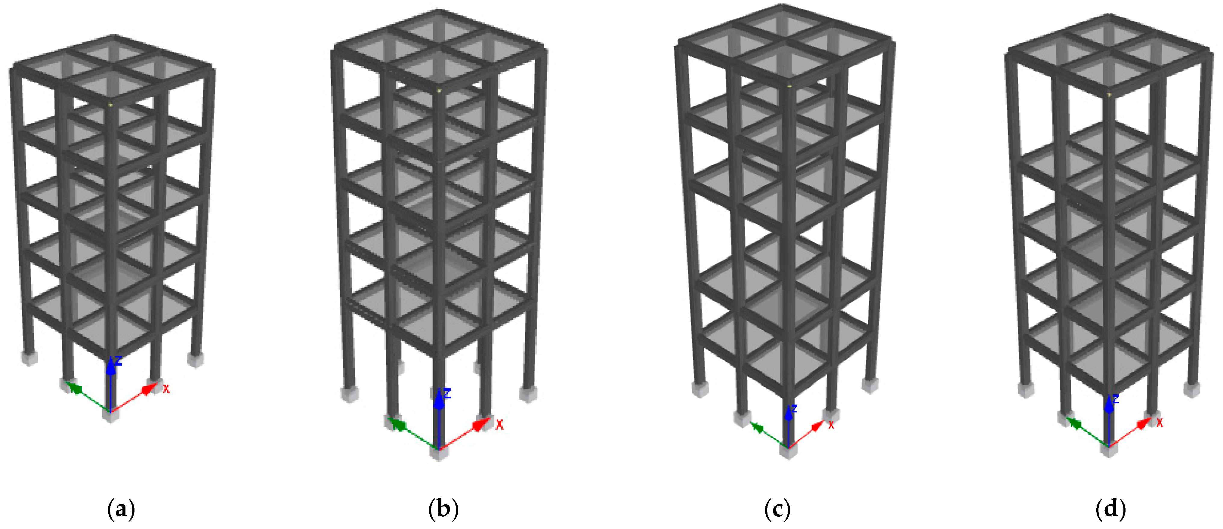
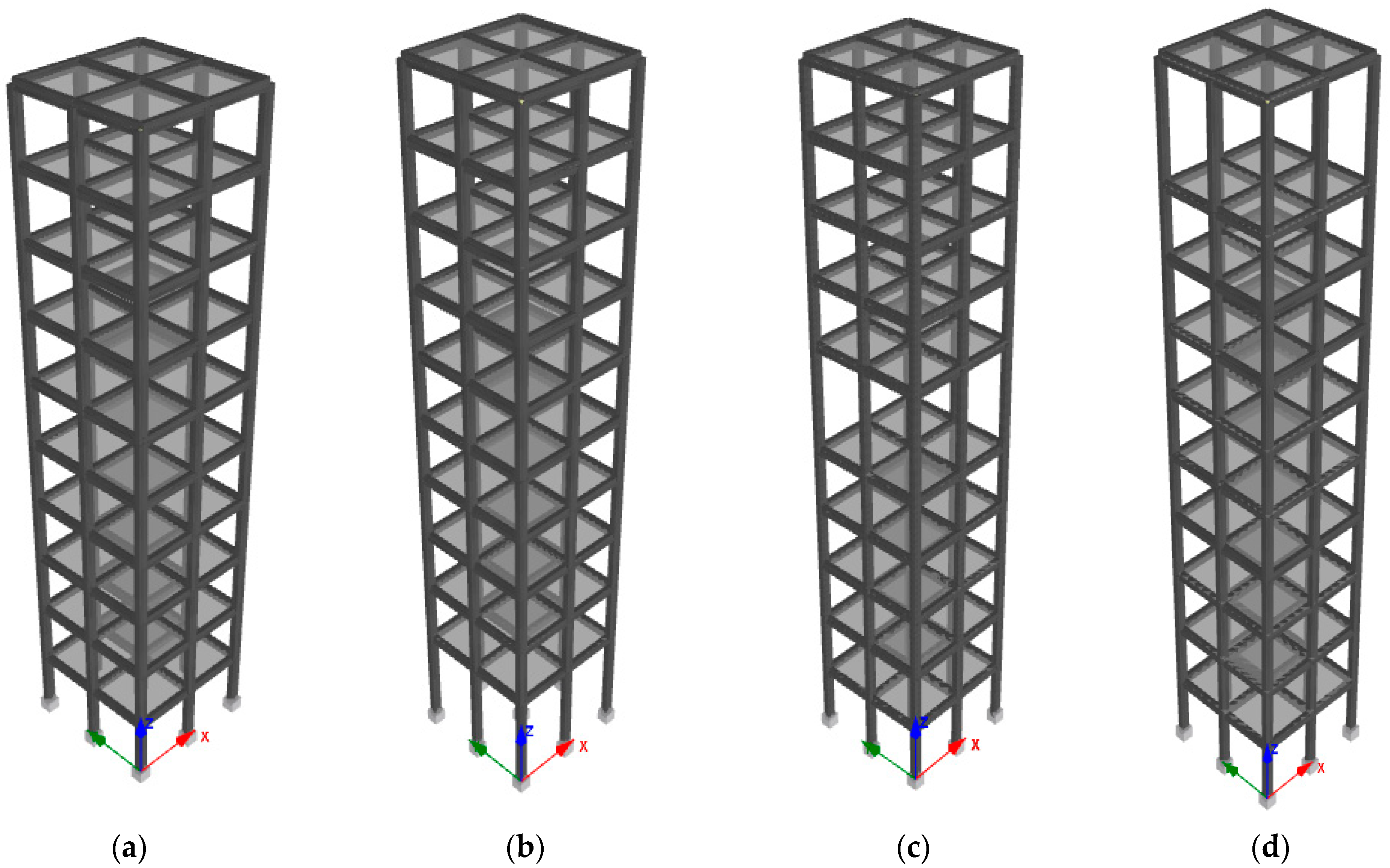
This study focuses on investigating a series of reinforced concrete (RC) structures with identical floor plans. Figure 1 illustrates the 3D structural models of the buildings under consideration, specifically a five- and a ten-story building. Without a soft story, the story height of each building (reference model) has been kept constant at 3 m. The chosen structures represent the dynamic behavior of medium- and high-rise buildings, respectively [16]. The structural models are considered to be RC moment-resisting frames (MRFs). In the case of soft-story buildings, it is anticipated that the soft-story level would possess one of two distinct heights, namely 5 m or 7 m. For all building models, a bay width of 3 m has been maintained. The ten-story and five-story reference models are defined in the current study as M_10ref and M_5ref, respectively. In the building models under consideration, it is presumable that the soft story will be provided at the top, middle, and bottom levels. Soft stories with 5 m height at the top, middle, and bottom levels of a five-story model are labelled as M_5ts5, M_5ms5, and M_5bs5, respectively, as shown in Figure 1b–d. Similarly, soft stories with a 7 m height at the top, middle, and bottom levels of a five-story model are labelled as M_5ts7, M_5ms7, and M_5bs7, respectively. The M_10ts5, M_10ms5, and M_10bs5 configurations, which correspond to a 5 m soft story on the top, sixth, and bottom floor levels, respectively, are shown in Figure 2. Moreover, the soft-story height for the M_10bs7, M_10ms7, and M_10ts7 types is 7 m. The soft-story buildings meet the IS 1893(Part 1) 2016 [57] irregularity requirements. According to the IS 1893 standard, the stiffness irregularity checks, $K_i/K_{i+1}$ (ratio of lateral stiffness of $i^{th}$ to ${(i+1)}^{th}$ story), are performed in both plan directions, and the relevant values are provided in

Table 1. Building model stiffness irregularity ratios.

Model	Soft-Story Height (m)	Location of Soft Story (Floor Level)	${\mathit{K}}_{\mathit{i}}/{\mathit{K}}_{\mathit{i}+1}$
			X-Dir	Y-Dir
M5bs5	5	1	0.495	0.373
M5ms5	5	3	0.407	0.334
M5ts5	5	5	0.348	0.302
M10bs5	5	1	0.522	0.389
M10ms5	5	6	0.449	0.365
M10ts5	5	10	0.330	0.305
M5bs7	7	1	0.231	0.159
M5ms7	7	3	0.211	0.154
M5ts7	7	5	0.173	0.134
M10bs7	7	1	0.245	0.168
M10ms7	7	6	0.235	0.172
M10ts7	7	10	0.188	0.151

. This particular study explored the effect of a soft story and its location on the floor response spectra. Previous researchers did not study this effect. Hence, the authors were limited to a linear analysis of simple regular buildings and NSCs under strong ground motions. This study serves as a preliminary investigation for future studies to obtain more generalized research outcomes by considering more complex structures.

For the purposes of modelling reinforced concrete, the concrete and steel grades M 30 and HYSD 415 are used. In accordance with IS 875-Part 2 [58], the floor finishes and live load have been set at 1.5 kN/m² and 3 kN/m², respectively. According to IS 1893–2016, seismic zone V is supposed to represent the location of the buildings. The minimum dimensions specified in IS 13920: 2016 [59] were used to determine the column and beam’s primary dimensions. For the frames, the dimensions of the beams and columns (230 mm × 450 mm and 300 mm × 450 mm) have remained constant. Stiffness irregularity can also be achieved by altering the sizes of columns. By maintaining uniform column sizes from the ground floor to the top floor in the software analysis, the authors aimed to simplify the input and reduce errors. In this research, the authors addressed vertical stiffness irregularities in the structure by adjusting the story heights to meet the criteria outlined in IS 1893–2016. The thickness of the RC slab is fixed at 150 mm for all the models. To evaluate the behavior of the models, the software SeismoStruct (2023 version) [60] was utilized to conduct a linear time–history analysis. This analysis focused on examining the bare frames’ elastic responses. The elastic model of the structure that is employed as a reference case aims to imitate the theoretical behavior of the structures while ignoring nonlinear effects during the dynamic response. The columns and beams are defined using the elastic frame element. Mander et al. [61] developed a model for defining the compression behavior of constrained concrete. The Menegotto–Pinto [62] steel model is used to account for the tension behavior of steel reinforcements. The penalty function nodal constraints approach is used to simulate RC slabs as a rigid diaphragm. The determination of the penalty function exponent for the building was based on the work conducted by Pinho et al. [63], and in this case it is 10¹⁰. To simulate the damping effects, a damping ratio (Rayleigh model) of 5% is established. The method used for the numerical modelling and analysis of 3D buildings has been experimentally validated by the software developer. A verification report [64] compares the seismic responses of RC buildings from SeismoStruct simulations to experimental observations. Our current study on elastic 3D buildings employs similar methods to those detailed in the mentioned report [64] and study [65].

In this study, the authors chose to analyze simple, regular buildings with soft stories at different levels. By opting for simplicity, they aimed to narrow down their focus to specific phenomena and fundamental behaviors. This approach allowed them to pinpoint the crucial factors influencing both the structural and non-structural responses of buildings with soft stories. By using these simplified models, the researchers were able to gain meaningful insights into how soft-story configurations impact the overall building performance (especially elastic floor acceleration demands) during seismic events. The building models used in this study are considered to be fixed to the ground, and therefore soil–structure interaction effects are not taken into account.

3. Selection and Scaling of Ground Motions

Realistic responses in the seismic reaction evaluation technique are produced using actual ground motion data [66,67]. The current study incorporated 11 horizontal ground motion excitations for hard soil types, which were obtained from the freely available NGA-West2 Database, PEER [68]. These ground motion recordings were selected in accordance with the guidelines outlined in ASCE 7–16 [33]. The NEHRP [34] site categorization scheme states that excitations are decided by referring to shear wave velocity (V_S30) to indicate hard soil.

Table 2. Ground motion information.

Earthquake	Year	Station	Mw	Rjb (km)	Vs30 (m/s)
Helena_ Montana-01	1935	Carroll College	6	2.07	593.35
Helena_ Montana-02	1935	Helena Fed Bldg	6	2.09	551.82
Kern County	1952	Pasadena—CIT Athenaeum	7.36	122.65	415.13
Kern County	1952	Santa Barbara Courthouse	7.36	81.3	514.99
Kern County	1952	Taft Lincoln School	7.36	38.42	385.43
Southern Calif	1952	San Luis Obispo	6	73.35	493.5
Parkfield	1966	Cholame—Shandon Array #12	6.19	17.64	408.93
Parkfield	1966	San Luis Obispo	6.19	63.34	493.5
Parkfield	1966	Temblor pre-1969	6.19	15.96	527.92
Borrego Mtn	1968	Pasadena—CIT Athenaeum	6.63	207.14	415.13
Borrego Mtn	1968	San Onofre—So Cal Edison	6.63	129.11	442.88

displays the specifics of the excitations. For this investigation, ground motions compatible with the design spectrum were chosen, since they can significantly save computational time [69]. In order to generate seismic excitations that are compatible with the spectral characteristics of the desired response spectrum, the time domain spectral matching method proposed by reference [70] is utilized.

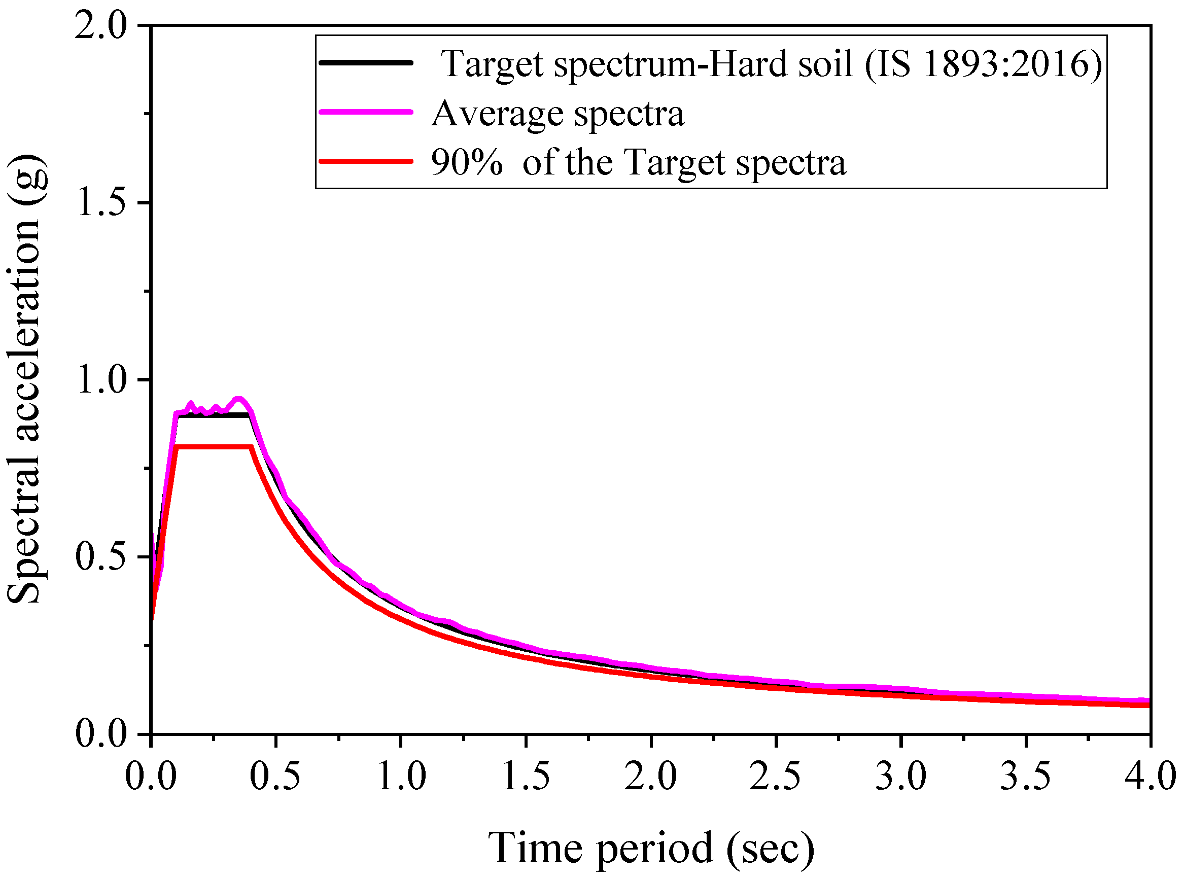
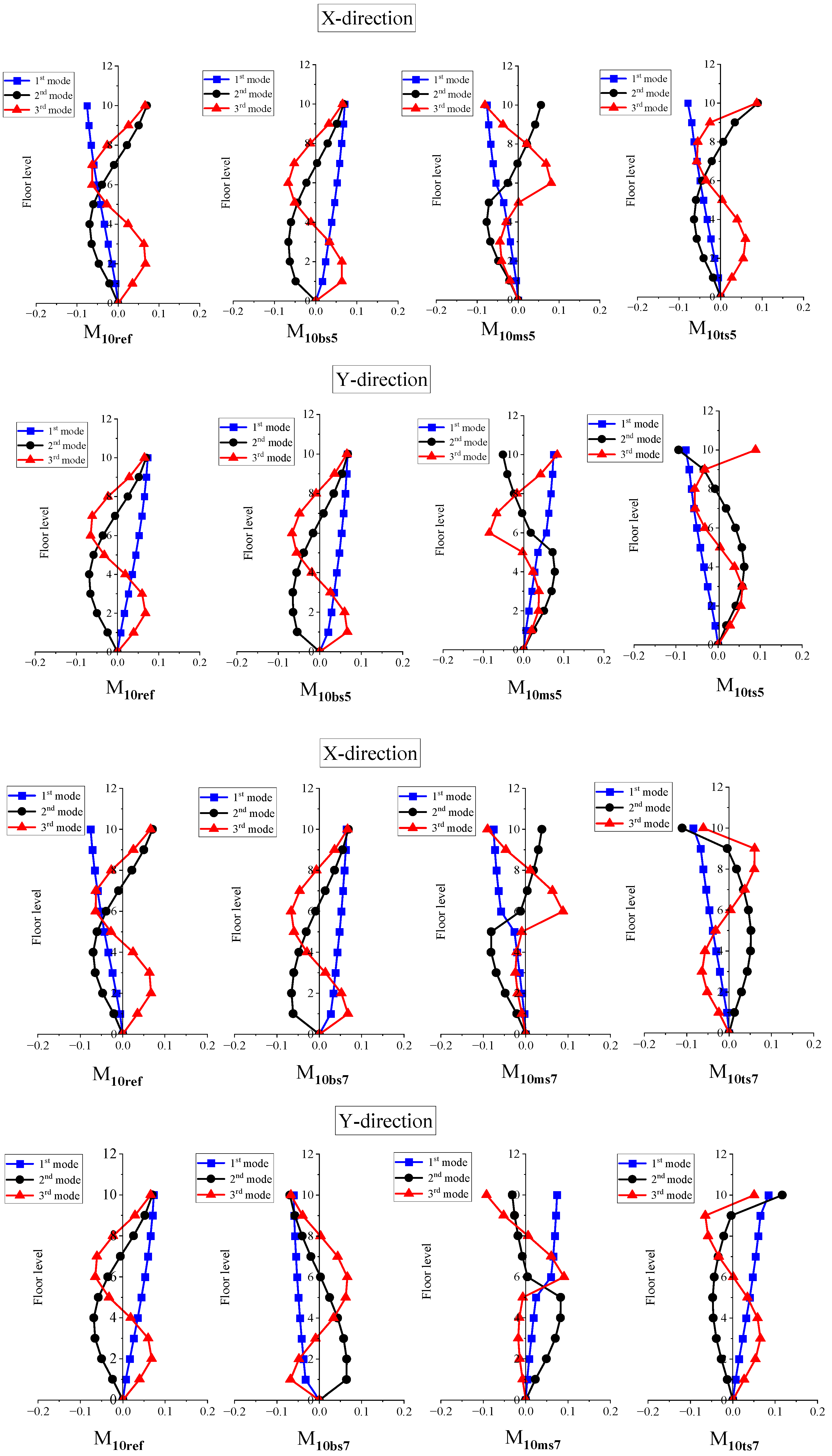
The mean ground excitation spectra and the target spectra for IS 1893:2016, associated with 5% damping, are shown in Figure 3. The analysis of Figure 3 reveals a clear distinction, as the mean spectra illustrated in the figure substantially surpass 90% of the target spectra as per ASCE 7–16 guidelines. This observation suggests that the mean ground excitation spectra, as represented in Figure 3, meets the requirements set forth by the ASCE 7–16 guidelines, indicating a satisfactory level of seismic performance for the analyzed structure. The first three mode shapes of the models in both directions are shown in Figure 4 and Figure 5. The modal periods are shown in

Table 3. Five-story models: modal periods (seconds).

Mode	M5ref	M5bs5	M5ms5	M5ts5	M5bs7	M5ms7	M5ts7
1st Mode (Y)	0.54	0.76	0.71	0.59	1.11	0.96	0.67
2nd Mode (X)	0.44	0.58	0.56	0.47	0.81	0.73	0.53
3rd Mode (R)	0.42	0.56	0.53	0.45	0.76	0.68	0.5
4th Mode (Y)	0.18	0.23	0.2	0.25	0.25	0.22	0.34
5th Mode (X)	0.14	0.18	0.16	0.19	0.20	0.17	0.25
6th Mode (R)	0.13	0.17	0.15	0.18	0.19	0.16	0.24
7th Mode (Y)	0.10	0.12	0.14	0.14	0.13	0.15	0.14
8th Mode (X)	0.08	0.10	0.10	0.11	0.10	0.12	0.11
9th Mode (R)	0.07	0.09	0.09	0.10	0.09	0.11	0.10
10th Mode (Y)	0.06	0.08	0.08	0.09	0.08	0.08	0.08
11th Mode (X)	0.05	0.06	0.07	0.07	0.07	0.07	0.06
12th Mode (R)	0.11	0.05	0.06	0.06	0.06	0.06	0.05

(five-story) and

Table 4. Ten-story building models: modal periods (seconds).

Mode	M10ref	M10bs5	M10ms5	M10ts5	M10bs7	M10ms7	M10ts7
1st Mode (Y)	1.13	1.37	1.28	1.16	1.77	1.54	1.20
2nd Mode (X)	0.94	1.11	1.06	0.98	1.37	1.24	1.01
3rd Mode (R)	0.83	0.98	0.93	0.85	1.21	1.07	0.87
4th Mode (Y)	0.37	0.45	0.41	0.40	0.52	0.46	0.49
5th Mode (X)	0.30	0.36	0.33	0.33	0.42	0.36	0.38
6th Mode (R)	0.27	0.32	0.31	0.29	0.36	0.35	0.35
7th Mode (Y)	0.21	0.24	0.24	0.25	0.25	0.26	0.30
8th Mode (X)	0.17	0.19	0.19	0.19	0.20	0.21	0.23
9th Mode (R)	0.16	0.18	0.18	0.18	0.19	0.19	0.23
10th Mode (Y)	0.15	0.16	0.17	0.17	0.17	0.18	0.18
11th Mode (X)	0.12	0.13	0.13	0.14	0.14	0.14	0.15
12th Mode (R)	0.11	0.12	0.12	0.13	0.13	0.13	0.14

(ten-story). The modal mass participation (cumulative) percentages are displayed in

Table 5. (a) Cumulative modal mass participation ratio of five-story buildings (soft-story height = 5 m). (b) Cumulative modal mass participation ratio of five-story buildings (soft-story height = 7 m).

(a)
Mode	M5ref		M5bs5		M5ms5		M5ts5
	$\mathit{U}\mathit{X}$	$\mathit{U}\mathit{Y}$	$\mathit{U}\mathit{X}$	$\mathit{U}\mathit{Y}$	$\mathit{U}\mathit{X}$	$\mathit{U}\mathit{Y}$	$\mathit{U}\mathit{X}$	$\mathit{U}\mathit{Y}$
First Mode (Y)	0	84.9	0	96.0	0	76	0	80.1
Second Mode (X)	83	84.9	94.0	96.0	76.3	76	78.7	80.1
Third Mode (R)	83	84.9	94.0	96.0	76.3	76	78.7	80.1
Fourth Mode (Y)	83	95.1	94.0	99.5	76.3	95.6	78.7	91.2
Fifth Mode (X)	94	95.1	99.2	99.5	94.7	95.6	90.4	91.2
Sixth Mode (R)	94	95.1	99.2	99.5	94.7	95.6	90.4	91.2
Seventh Mode (Y)	94	98.3	99.2	99.9	94.7	96.9	90.4	97.2
Eighth Mode (X)	94	98.3	99.2	99.9	97.0	96.9	90.4	97.2
Ninth Mode (R)	97.8	98.3	99.8	99.9	97.0	96.9	96.6	97.2
Tenth Mode (Y)	97.8	99.6	99.8	99.9	97.0	99.6	96.6	99.9
Eleventh Mode (X)	97.8	100	99.8	99.9	97.0	99.6	96.6	99.9
Twelfth Mode (R)	97.8	100	99.8	99.9	97.0	99.6	96.6	99.9
(b)
Mode	M5ref		M5bs7		M5ms7		M5ts7
	$\mathit{U}\mathit{X}$	$\mathit{U}\mathit{Y}$	$\mathit{U}\mathit{X}$	$\mathit{U}\mathit{Y}$	$\mathit{U}\mathit{X}$	$\mathit{U}\mathit{Y}$	$\mathit{U}\mathit{X}$	$\mathit{U}\mathit{Y}$
First Mode (Y)	0	84.9	0	99.0	0	68.8	0	80.1
Second Mode (X)	83	84.9	98.1	99.0	69.7	68.8	78.7	80.1
Third Mode (R)	83	84.9	98.1	99.0	69.7	68.8	78.7	80.1
Fourth Mode (Y)	83	95.1	98.1	99.9	69.7	96.6	78.7	91.2
Fifth Mode (X)	94	95.1	99.8	99.9	69.7	96.6	90.4	91.2
Sixth Mode (R)	94	95.1	99.8	99.9	95.5	96.6	90.4	91.2
Seventh Mode (Y)	94	98.3	99.8	99.9	95.5	96.9	90.4	97.2
Eighth Mode (X)	94	98.3	99.9	99.9	96.4	96.9	90.4	97.2
Ninth Mode (R)	97.8	98.3	99.9	99.9	96.4	96.9	96.6	97.2
Tenth Mode (Y)	97.8	99.6	99.9	100	96.4	99.9	96.6	99.4
Eleventh Mode (X)	97.8	100	99.9	100	96.4	100	96.6	99.9
Twelfth Mode (R)	97.8	100	99.9	100	96.4	100	96.6	99.9

and

Table 6. (a) Cumulative modal mass participation ratio of ten-story buildings (soft-story height = 5 m). (b) Cumulative modal mass participation ratio of ten-story buildings (soft-story height = 7 m).

(a)
Mode	M10ref		M10bs5		M10ms5		M10ts5
	$\mathit{U}\mathit{X}$	$\mathit{U}\mathit{Y}$	$\mathit{U}\mathit{X}$	$\mathit{U}\mathit{Y}$	$\mathit{U}\mathit{X}$	$\mathit{U}\mathit{Y}$	$\mathit{U}\mathit{X}$	$\mathit{U}\mathit{Y}$
First Mode (Y)	0	80.7	0	90.3	0	75.5	0	79.8
Second Mode (X)	78.6	80.7	87.0	90.3	74.5	75.5	77.8	79.8
Third Mode (R)	78.6	80.7	87.0	90.3	74.5	75.5	77.8	79.8
Fourth Mode (Y)	78.6	92.3	87.0	98.9	74.5	92.6	77.8	90. 9
Fifth Mode (X)	91.3	92.3	97.5	98.9	91.6	92.6	90.1	90. 9
Sixth Mode (R)	91.3	92.3	97.5	98.9	91.6	92.6	90.1	90.9
Seventh Mode (Y)	91.3	95.8	97.5	100	91.6	93.9	90.1	94.4
Eighth Mode (X)	95.0	95.8	99.1	100	93.4	93.9	93.9	94.4
Ninth Mode (R)	95.0	95.8	99.1	100	93.4	93.9	93.9	94.4
Tenth Mode (Y)	95.0	97.5	99.1	100	93.4	97.6	93.9	96.8
Eleventh Mode (X)	95.0	98.6	99.6	100	97.1	97.6	96.3	96.8
Twelfth Mode (R)	97.0	98.6	99.6	100	97.1	97.6	96.3	96.8
(b)
Mode	M10ref		M10bs7		M10ms7		M10ts7
	$\mathit{U}\mathit{X}$	$\mathit{U}\mathit{Y}$	$\mathit{U}\mathit{X}$	$\mathit{U}\mathit{Y}$	$\mathit{U}\mathit{X}$	$\mathit{U}\mathit{Y}$	$\mathit{U}\mathit{X}$	$\mathit{U}\mathit{Y}$
First Mode (Y)	0	80.7	0	96.4	0	68.5	0	77.7
Second Mode (X)	78.6	80.7	93.8	96.4	69.1	68.5	76.1	77.7
Third Mode (R)	78.6	80.7	93.8	96.4	69.1	68.5	76.1	77.7
Fourth Mode (Y)	78.6	92.3	93.8	99.6	69.1	92.7	76.1	87.2
Fifth Mode (X)	91.3	92.3	99.4	99.6	91.9	92.7	87.1	87.2
Sixth Mode (R)	91.3	92.3	99.4	99.6	91.9	92.7	87.1	87.2
Seventh Mode (Y)	91.3	95.8	99.4	99.8	91.9	92.9	87.1	93.7
Eighth Mode (X)	95.0	95.8	99.8	99.8	92.3	92.9	93.0	93.7
Ninth Mode (R)	95.0	95.8	99.8	99.8	92.3	92.9	93.0	93.7
Tenth Mode (Y)	95.0	97.5	99.8	99.9	92.3	97.5	93.0	96.6
Eleventh Mode (X)	95.0	98.6	99.9	99.9	97.1	97.5	96.0	96.6
Twelfth Mode (R)	97.0	98.6	99.9	99.9	97.1	97.5	96.0	96.6

.

4. Results and Discussion

The next sections demonstrate how various response parameters affect the behavior of the non-structural components. CDAFs and FRSs are parameters that precisely define the behavior of NSCs, and are clearly displayed in the X and Y directions individually because of the use of bi-directional ground motion. For the sake of concision, the response parameters are only examined for the first, third, fifth, sixth, eighth, and tenth story levels of the ten-story building models.

4.1. Peak Floor Acceleration (PFA)

Soft-story building models have higher floor acceleration amplification at both the bottom and top soft-story levels in orthogonal directions compared to the reference building models. In the X direction, for example, the ratio of $PFA⁄PGA$ increases by 39.7% and 26.1% for the bottom floor of model M_5bs with soft-story heights of 5 m and 7 m, respectively, compared to model M_5ref. Similarly, the top floor of M_5ts shows a raise of 9.1% and 7.2% in the ratio of PFA⁄PGA for soft-story heights of 5 m and 7 m, respectively, compared to M_5ref. For M_10bs, the ratio of $PFA⁄PGA$ in the bottom floor increases by 62.6% and 85.5% for soft-story heights of 5 m and 7 m, respectively, in the X direction, compared to model M_10ref. Additionally, the top floor of M_10ts experiences increases of 22.2% and 24.1% in the ratio of PFA⁄PGA for soft-story heights of 5 m and 7 m, respectively, in the X direction, compared to M_10ref.

In the middle soft-story building model, floors below the soft-story level show higher floor acceleration amplification compared to the reference building models. For example, in the five-story middle soft-story building, the second-floor experiences increase of 14% and 11.8% in the ratio of $PFA⁄PGA$ for soft-story heights of 5 m and 7 m, respectively, in the X direction, compared to the reference building. Similarly, in the ten-story building model, the fifth-floor shows increases of 22.8% and 54.2% in the ratio of $PFA⁄PGA$ for soft-story heights of 5 m and 7 m, respectively, in the X direction, compared to the reference building. This indicates that the location of a soft story significantly influences peak floor accelerations.

Different seismic codes, such as ASCE 7–16 [33] and Eurocode 8 [71], offer formulas to evaluate the variations in peak floor acceleration concerning the building’s height. The floor amplification factor ($PFA/PGA$) is determined using Equations (1) and (2) for these codes.

$$PFA/PGA=1+2\frac{z}{h}$$

(1)

$$PFA/PGA=1+1.5\frac{z}{h}$$

(2)

Figure 6 reveals that the code formulations suggest a linear relationship between the floor amplification and the building height. However, the analysis shows that floor acceleration varies nonlinearly throughout the building height. Additionally, the code formulations underestimate the floor acceleration demands at soft-story levels in all building models considered. This suggests that the linear hypothesis in the code-based formulas may lead to the underestimation or overestimation of floor acceleration demands. To improve accuracy, the current code-based formulas could be modified to consider the effects of vertical stiffness irregularity, which influences floor acceleration demands. In summary, the code-based formulations do not adequately predict the peak responses of non-structural components with respect to building height.

4.2. Floor Response Spectra (FRSs)

This section and the results presented here are based on past research [72], and they have been reproduced here to enhance readability and facilitate comprehension for the readers. The considered NSCs are elastic single degree of freedom (SDOF) systems with masses much smaller than the supporting structure. They have a single attachment point to the floor, and the dynamic interaction effects with the structure can be disregarded. The FRS technique decouples and independently assesses NSCs and structure in a predefined manner. For NSCs to create the appropriate FRSs, absolute acceleration data are collected from each floor’s model separately. The floor response spectra for each of the models taken into consideration were derived in the manner that was previously indicated. For each ground motion, the acceleration response is recorded at multiple floor levels to obtain FRSs. The mean findings are displayed for each floor and were achieved at a damping ratio of 5%.

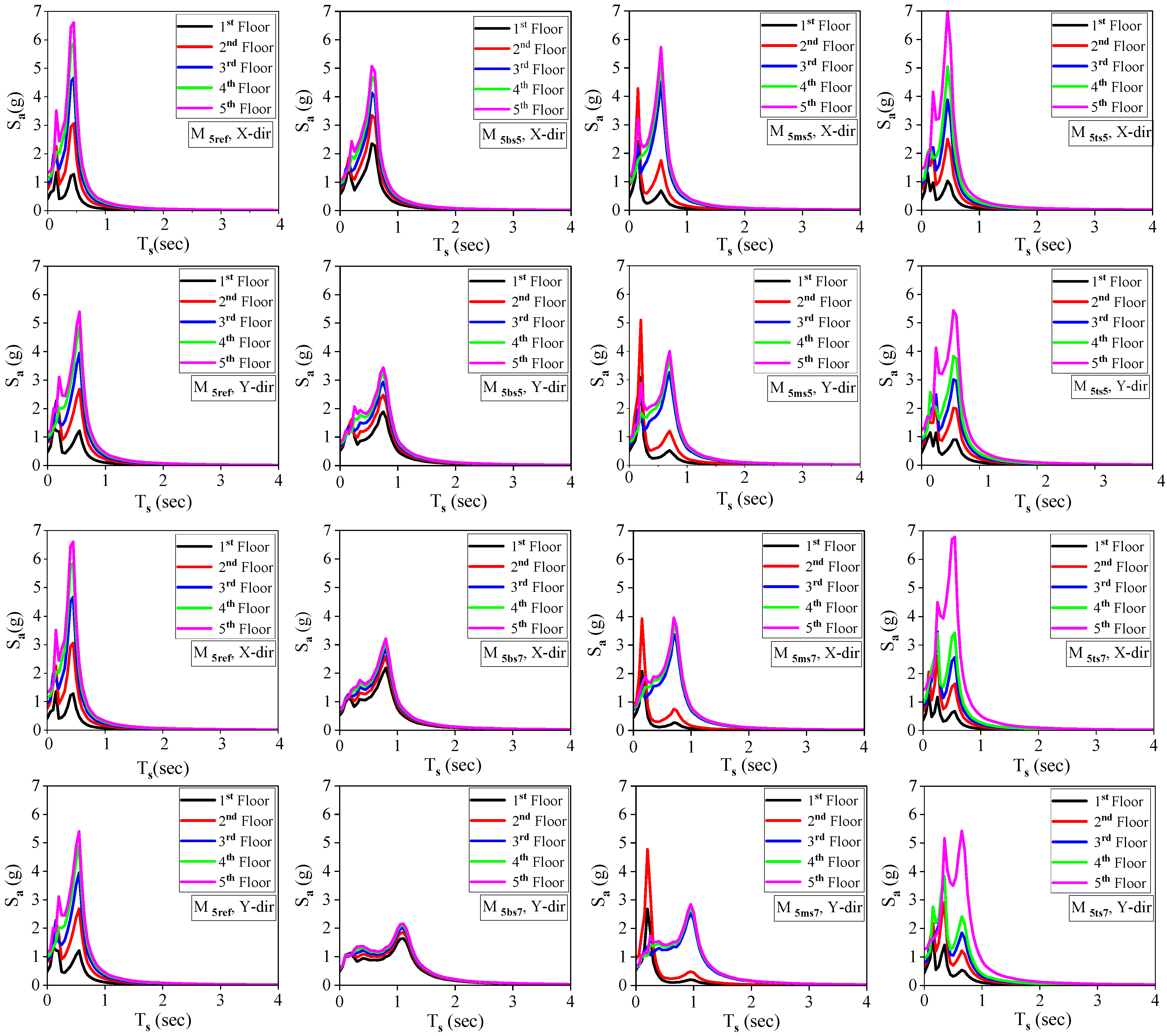
Figure 7 and Figure 8 display the relationship between the vibration period of a non-structural component ($T_s$ in seconds) and the peak spectral acceleration ($S_a$ in $g$) of the floor. When the FRS is plotted throughout a wide variety of periods, maximum spectrum peaks should appear at the fundamental natural period of the supporting structure [73]. FRS peaks align with the typical periods of relevant building models. In all considered models, spectral accelerations are higher in the X direction for the first modal period. Increasing the soft-story height (from 5 m to 7 m) decreases FRS amplitudes across all floor levels. In all the models, the FRS intensity decreases from the upper fifth story to the lower first level. The soft story’s presence and location have a notable impact on the FRS, as evident from the FRS curves depicted in Figure 7 and Figure 8. In a M_5ref, the FRS exhibits two peaks corresponding to the first and second modal periods for the first and second floor levels. The impact of the higher mode is negligible for the higher floors (third, fourth, and fifth). This observation aligns with previous research findings [16]. Peak spectral acceleration related to the higher modes increases with increasing building height (ten-story reference building). Up to the third floor, the second and thirds modes significantly influence the peaks of FRSs, whereas the higher mode’s contribution has less of an impact as the floor levels increase. This observation confirms the findings of Vukobratovi’c and Ruggieri [19]. Consequently, it can be deduced that, in the absence of vertical stiffness irregularities, short-period NSCs located in the lower floors of a building would experience significant earthquake forces.

A noticeable amplification of spectral accelerations between floors can be observed with a 5m soft story. The spectra of the levels begin to converge as the height of a soft story increases to 7m. In model M_5bs5, the peak spectral acceleration at the first modal period of the bottom level (first floor) experiences significant increases of 79% in the X direction and 55.3% in the Y direction. Corresponding to this, in M_10bs5, the $S_a$, associated with the second modal period, is amplified by 67.9% and 48.6% in the X and Y directions, respectively, when compared to M_10ref. As compared to M_5ref, the model M_5bs7’s spectral acceleration increased by 71.6% and 33%, respectively, in both the X and Y directions. The $S_a$ of the top floor for the first modal period is higher in both the directions of excitation in model M_5ts5 compared to M_5ref. It increases by 6.36% and 0.55%, respectively. In the M_10ts5 configuration, the $S_a$ for the second modal period increases by 23.28% in the X direction and 49.8% in the Y direction compared to the M_10ref configuration. In the M_5ts7 model, the spectral acceleration increases by 2.72% in the X direction and 0.37% in the Y direction compared to M_5ref.

The inclusion of a middle soft story in building models significantly affects the peak floor spectral acceleration directly below the soft story (second floor in five-story models and fifth floor in ten-story models). In the X direction, the $S_a$ of the second floor in model M_5ms5 is decreased by 42.8% for the first modal period, and increased by 89.7% for the second modal period compared to M_5ref. In the M_10ms5 configuration, the $S_a$ of the fifth floor, associated with the second modal period, increases by 21.6% compared to M_10ref. Hence, for buildings with a middle soft story, it is recommended to add a component matching the first modal period’s vibration to floors underneath the soft story, as the first mode of vibration has minimal impact.

4.3. Component Dynamic Amplification Factor

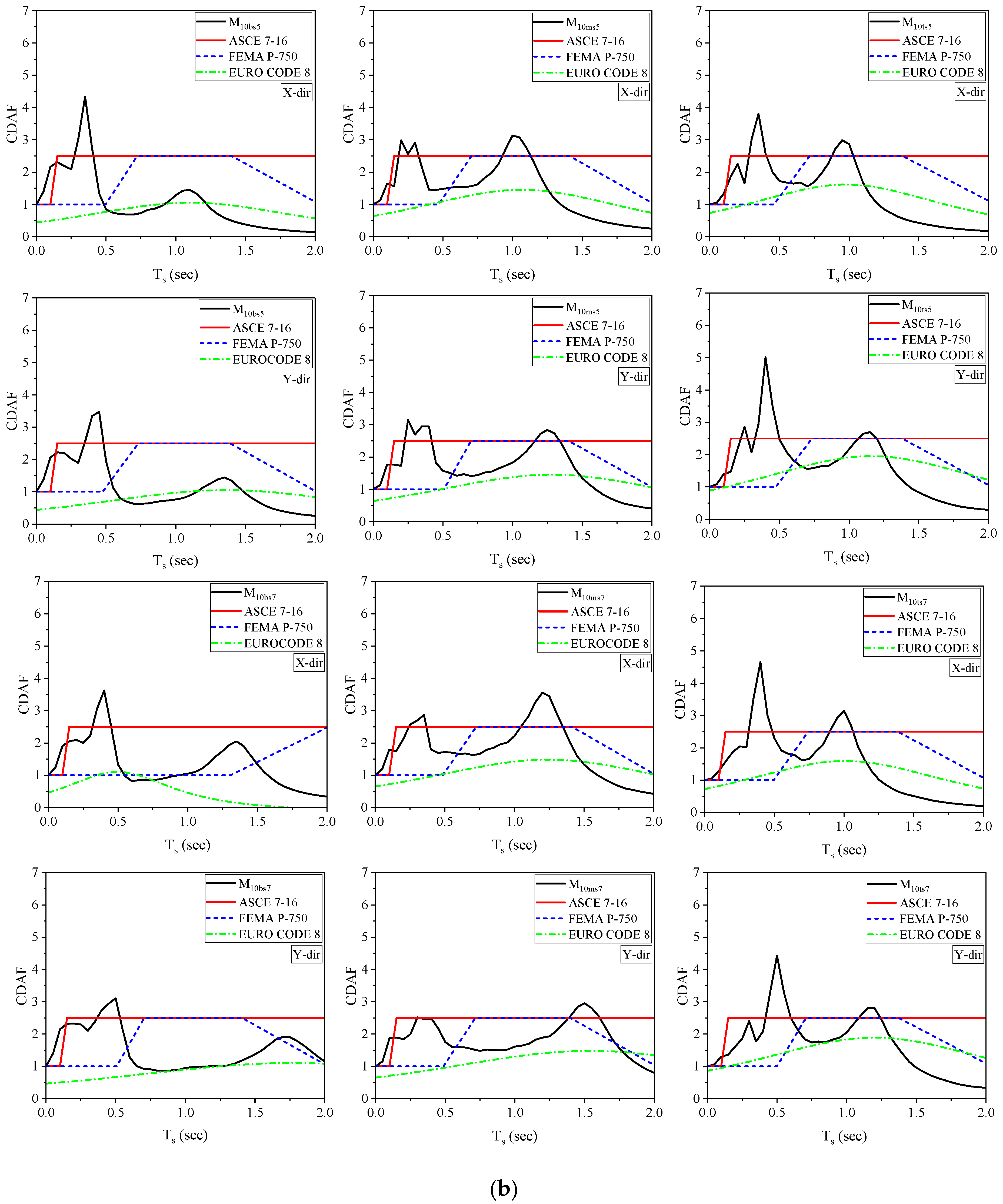
This section and its results are derived from previous research [72], reproduced here to improve readability and aid reader comprehension. This section aims to analyze the acceleration of the NSC in relation to the floor acceleration. All the building models that are being examined have their story FRSs normalized based on the associated peak floor accelerations (PFAs). Figure 9 displays the soft-story FRSs, normalized based on the relevant PFAs. The CDAF is denoted by the ratio $FRS/PFA$. In this study, the CDAFs of the building models are compared to the criteria of ASCE 7–16 [33], FEMA P-750 [34], and Eurocode 8 [71].

In medium soft-story buildings, the amplification factor ranges from 3.55 to 4.92, correlating with the NSCs’ fundamental vibration period. For bottom-soft-story models, the amplification factors range from 1.37 to 4.07, while top-soft-story models have values between 2.69 and 4.79. Overall, buildings with a soft story at the middle floor experience the highest amplification in the acceleration of the NSC. Figure 9 shows that the CDAF deviates from the definitions provided in FEMA P-750, ASCE 7, and Eurocode 8. This disparity becomes more noticeable as the time periods approach the vibration periods of the building models under investigation.

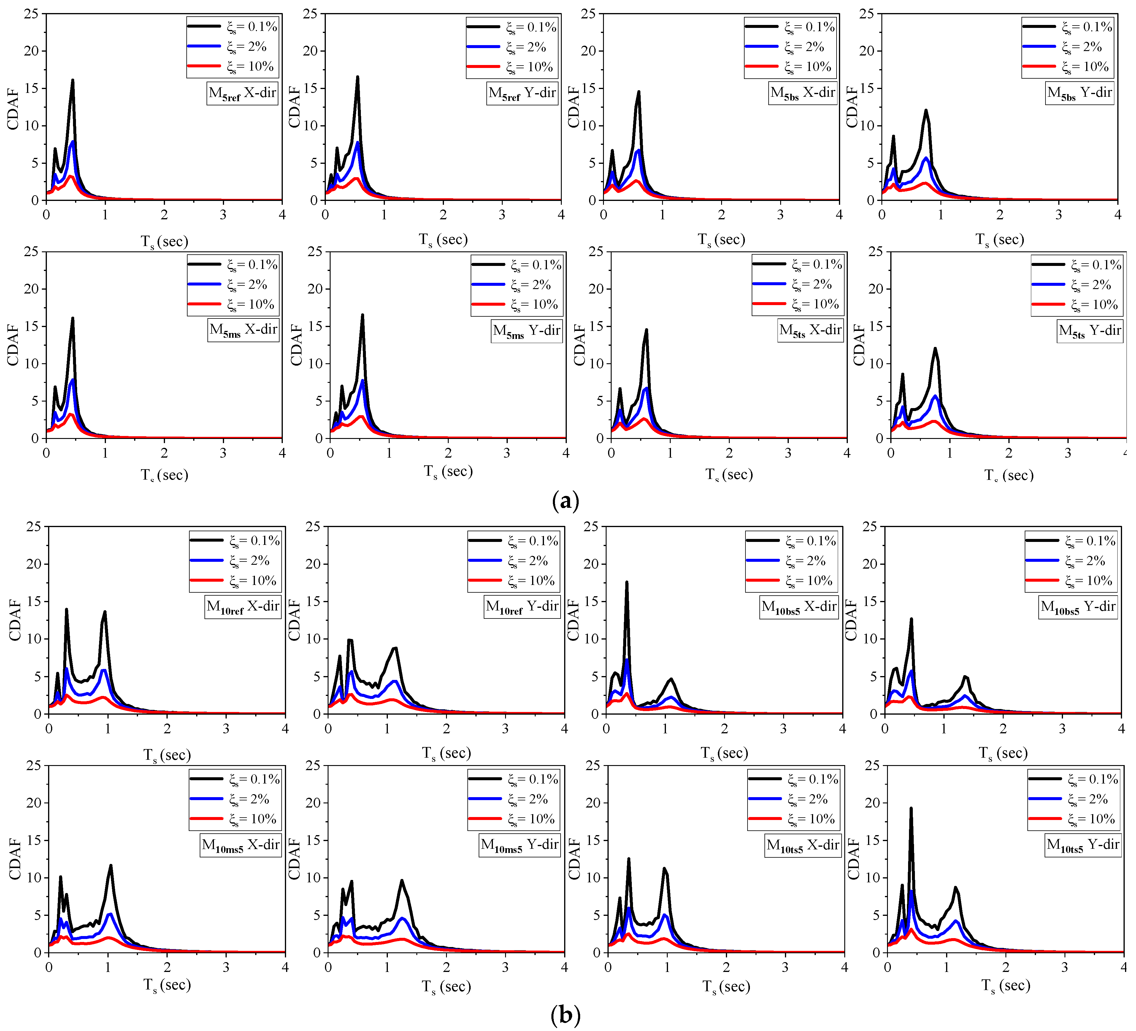
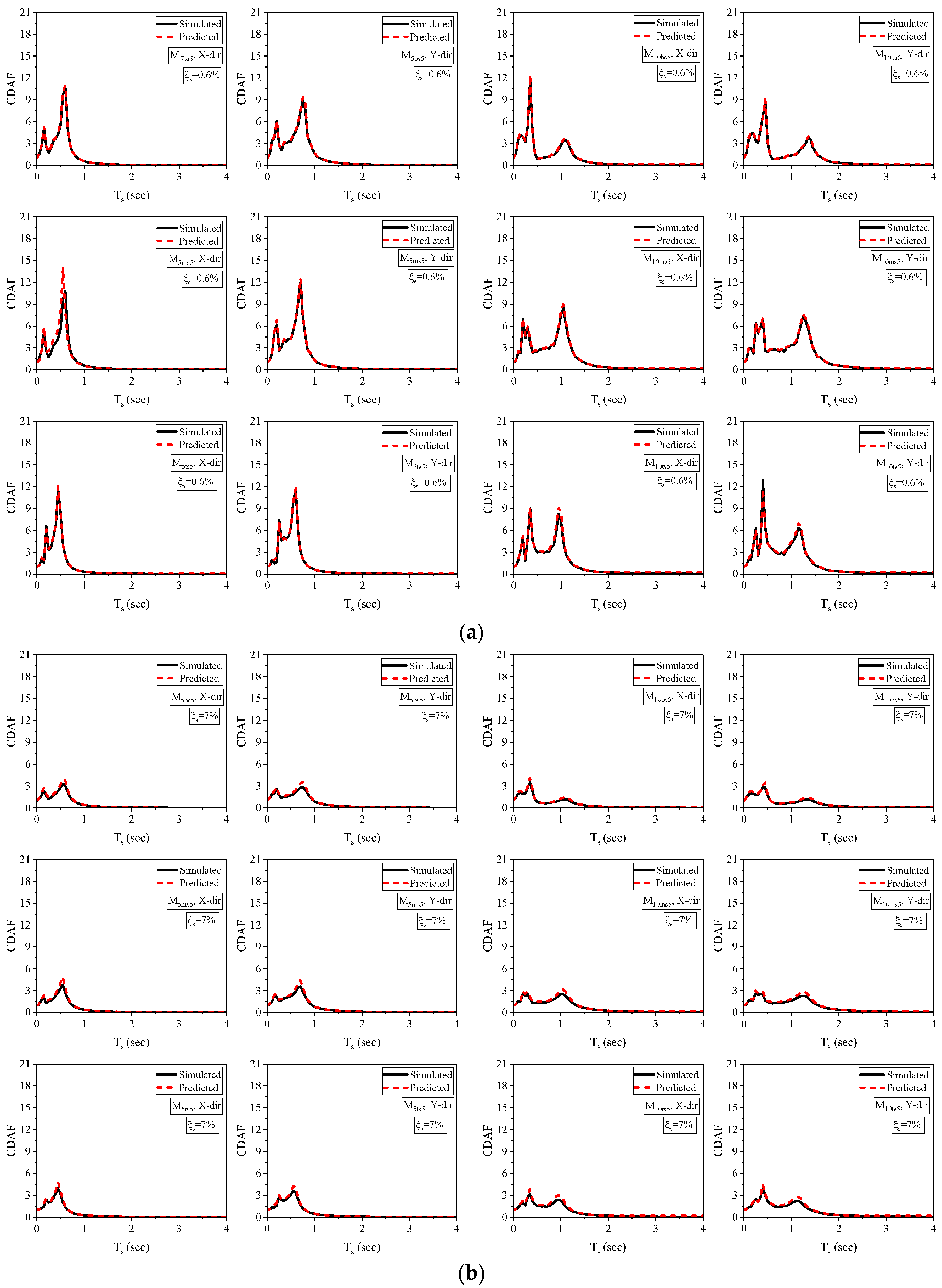
Considering the varying periods and damping ratios (${\xi }_s$) of non-structural components (NSCs), it becomes crucial to assess the influence of these characteristics on seismic behavior [74]. Therefore, this study evaluates CDAFs for different ${\xi }_s$ values (0.1%, 0.2%, 0.5%, 1%, 2%, 5%, and 10%). The CDAF spectrum for five- and ten-story models for various damping ratios (0.1%, 2%, and 10%) at the top floor (in the case of the reference structure) and soft-story floor level (in the case of other buildings) are shown in Figure 10. As predicted, lower damping ratios (${\xi }_s$) corresponded to higher amplification factor values. The damping ratio of the NSCs played a more substantial role in influencing the amplification factors, particularly at the modal periods of the models. 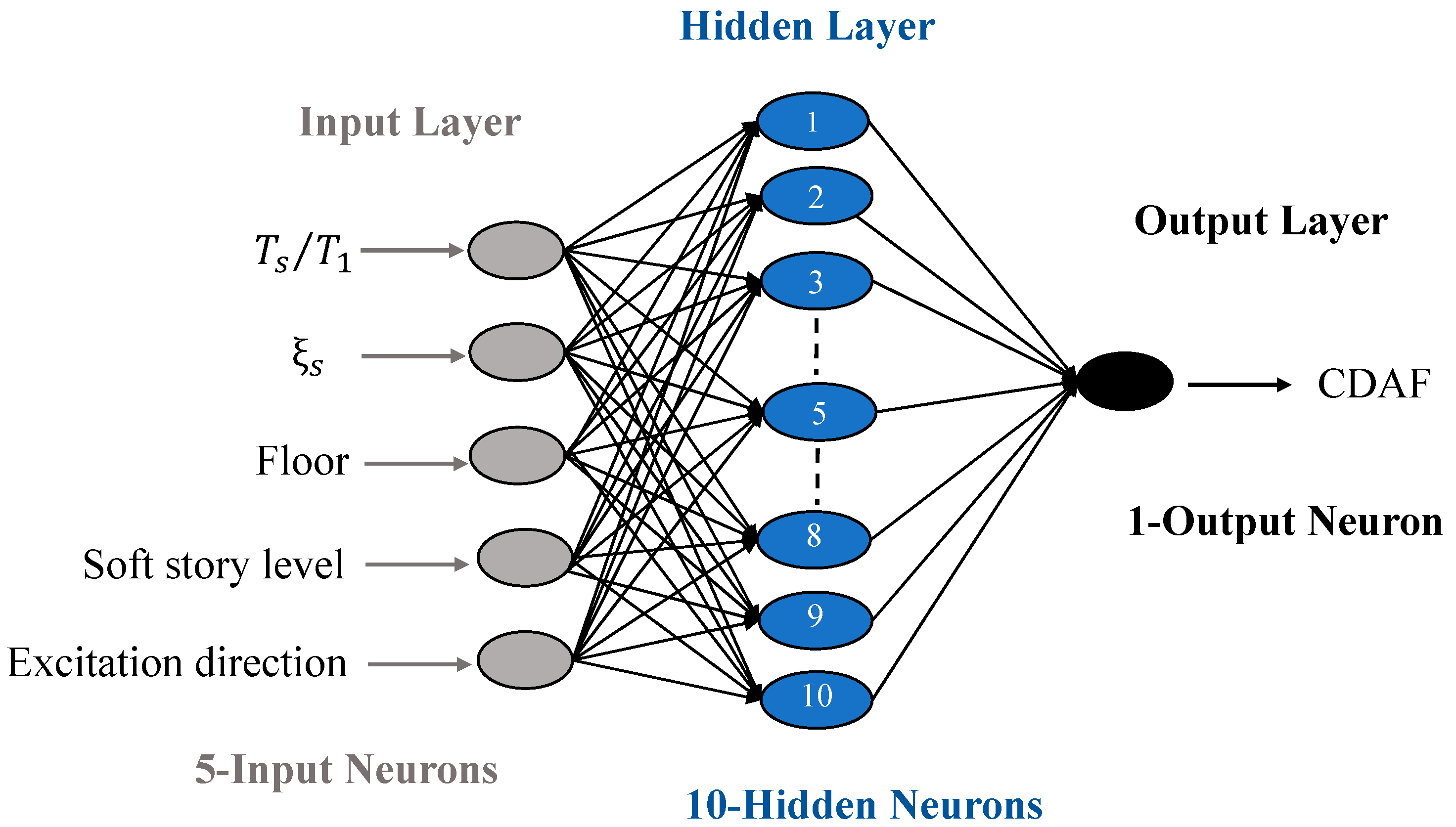Surprisingly, the impact of ${\xi }_s$ was found to be insignificant for very short and extremely long vibration periods. Therefore, this study aimed to develop a machine learning-based prediction model for the component dynamic amplification factor (CDAF) spectrum.

5. Machine Learning Models

Machine learning (ML) techniques have recently been widely employed to forecast the outcomes of diverse structural engineering issues [8,36,37]. In this study, the ML model is utilized to examine the performance of NSCs and assess their ability to establish a functional relationship between the given inputs and output. Thus, two popular supervised ML techniques were implemented in this study, namely the ANN model and RF model.

5.1. Data Analysis

The model takes into account various inputs, such as the tuning ratio ($T_s/T_1$), ${\xi }_s$, floor level, soft-story level, and excitation direction. These inputs are used to predict the corresponding CDAF values, which serve as the model’s output. The statistical characteristics of the input parameters can be summarized as follows: $(T_s/T_1$) ranged between 0 and 4.587 for five-story models and varied between 0 and 2.125 for ten-story models; ${\xi }_s$ ranged between 0.1% and 10%; five and ten floors for the five- and ten-story buildings, respectively; four soft-story conditions are considered (where 0, 1, 2, and 3 are assigned to reference, bottom, middle, and top soft-story models, respectively); two excitation directions (where, 0 and 1 are assigned to two orthogonal directions (X and Y), respectively). Figure 11 shows the statistical distributions of the input parameters generated from dataset of both five- and ten-story buildings.

Table 7. Statistical characteristics of the dataset from five-story models.

	${\mathit{T}}_{\mathit{s}}/{\mathit{T}}_1$	${\mathit{\xi }}_{\mathit{s}}$	Floor	Soft-Story Level	Excitation Direction
count	11,480	11,480	11,480	11,480	11,480
mean	1.777	2.685	3	1.5	0.5
std	1.110	3.376	1.414	1.118	0.500
min	0	0.1	1	0	0
25%	0.850	0.2	2	0.75	0
50%	1.713	1	3	1.5	0.5
75%	2.611	5	4	2.25	1
max	4.587	10	5	3	1

and

Table 8. Statistical characteristics of the dataset from ten-story models.

	${\mathit{T}}_{\mathit{s}}/{\mathit{T}}_1$	${\mathit{\xi }}_{\mathit{s}}$	Floor	Soft-Story Level	Excitation Direction
count	22,960	22,960	22,960	22,960	22,960
mean	0.899	2.692	5.5	1.5	0.5
std	0.545	3.371	2.872	1.118	0.500
min	0	0.1	1	0	0
25%	0.430	0.2	3	0.75	0
50%	0.890	1	5.5	1.5	0.5
75%	1.333	5	8	2.25	1
max	2.125	10	10	3	1

represent the statistical characteristics of both five-story and ten-story models.

The correlation matrix, presented in

Table 9. Correlation matrix between pairs of input parameters (five-story models).

	Ts/T1	ξs (%)	Floor	Soft Story Level	Excitation Direction	CDAF
Ts/T1	1	8.9 × 10−17	−1 × 10−17	−0.0361	−0.1865	−0.5169
ξs (%)	8.9 × 10−17	1	2 × 10−17	−2.7 × 10−18	2.04 × 10−17	−0.1813
Floor	−1 × 10−17	1.7 × 10−17	1	0	0	0.084
Soft story level	−0.0362	−3 × 10−18	0	1	0	−0.0077
Excitation direction	−0.1865	2 × 10−17	0	0	1	0.0548
CDAF	−0.5169	−0.1813	0.084	−0.0077	0.0548	1

and

Table 10. Correlation matrix between pairs of input parameters (ten-story models).

	Ts/T1	ξs (%)	Floor	Soft Story Level	Excitation Direction	CDAF
Ts/T1	1	−4 × 10−17	8.3 × 10−18	−0.0108	−0.1535	−0.4
ξs (%)	−4 × 10−17	1	0.0018	4.6 × 10−18	−1.95 × 10−18	−0.2931
Floor	8.3 × 10−18	0.0018	1	0	0	0.2193
Soft story level	−0.0108	4.6 × 10−18	0	1	0	−0.0385
Excitation direction	−0.1536	−2 × 10−18	0	0	1	0.0347
CDAF	−0.4	−0.2931	0.2193	−0.0385	0.0347	1

, reveals noteworthy associations among the variables. Notably, the tuning ratio ($T_s/T_1$) exhibits the most pronounced negative correlations, reaching 0.516 (five-story) and 0.399 (ten-story), with CDAFs. Following this, ${\xi }_s$ displays correlations of 0.181 (five-story) and 0.293 (ten-story) with CDAFs. Regarding the floor and excitation direction, positive correlation coefficients are observed for CDAFs. In contrast, the soft-story level exhibits a negative correlation with CDAFs. This intricate interplay of correlations offers valuable insights into the relationships among the input variables under consideration.

5.2. ANN Model’s Architecture and Hyperparameter Tuning

Biological neural networks function as simplified constructs that offer an analytical depiction of artificial neural networks (ANNs). With their ability to handle large datasets, tackle complex problems, and navigate ambiguous situations, neural networks have proven to be more accurate tools for calculations and predictions compared to conventional computational methods [75,76,77,78]. The primary challenge in constructing this model lies in determining the optimal architecture, including the number of hidden layers, epochs, batch size, and more. While machine learning algorithms learn parameter values like node weights and biases through forward and backpropagation, there are additional parameters—known as hyperparameters—that control the learning process itself. Tuning these hyperparameters is crucial to ensure that the model effectively addresses the machine learning problem reliably. In this study, the trial-and-error method was employed to identify the most suitable hyperparameter combinations for various machine learning models. Through an iterative approach, trial and error proves its value by progressively refining hyperparameters. We initiated with a basic hyperparameter set, closely observed the outcomes of the performance measurement function, and fine-tuned them based on our observations. This method becomes especially practical when dealing with limited datasets, as advanced techniques like Bayesian optimization might falter due to data constraints. In such scenarios, trial and error emerges as a straightforward and effective alternative. In analogous prediction problems, several researchers have opted for trial-and-error methodologies to construct ANN-based prediction models in their research [79,80,81,82]. In our study, we comprehensively addressed all essential hyperparameters for optimizing the model, with the exception of the learning rate. Notably, the Levenberg–Marquardt (LM) algorithm introduces a distinct concept of a learning rate compared to conventional gradient descent-based approaches. Unlike the traditional fixed learning rate, the LM algorithm dynamically adapts step size using a damping factor, ensuring the effective navigation of the error surface for convergence.

Specifically, three types of neural networks were evaluated: function fitting neural networks, feedforward neural networks, and cascade forward neural networks. These networks utilized a range of training and transfer functions (with consistent transfer functions across hidden layers). The process began by fixing the network and transfer functions. Multiple training functions or backpropagation algorithms were tested to identify the optimal one. Subsequently, various transfer functions were explored based on the selected training function. This sequential approach ensured that the most appropriate combinations were chosen. The experimentation continued by altering the network function, repeating the process, and recording the hyperparameter set that yielded the lowest mean absolute percentage error ($MAPE$), root mean square error ($RMSE$), and the highest coefficient of determination ($R^2$). Refer to

Table 11. Optimal configuration of the ANN model.

Algorithm	Hyperparameter	Optimal Value
Artificial Neural Network (ANN)	Number of neurons in the input layer	5
	Number of hidden layers	1
	Number of output neuron	1
	Number of neurons in the hidden layer	10
	Training data	70%
	Testing data	30%
	Number of epochs	1000
	Activation function	tanh
	Loss functions	$RMSE$$, MAPE$

for the optimized values of the hyperparameters. Thus, in the current study, an accurate CDAF spectrum prediction is achieved using a two-layered feedforward neural network. Two layers are present, the output layer and the hidden layer. The accurate approximation of any function is possible in neural networks with a single hidden layer [83]. Therefore, when developing the ANN 5–10-1 model, the 10 neurons in the hidden layer were taken into account (Figure 12).

5.3. Development of the ANN-Based Prediction Model

This section outlines the methodology to be adhered to for the construction of the predictive model. To train the hidden neurons, an appropriate learning technique must be created. The network is trained using the Levenberg–Marquardt (LM) variant of the backpropagation (BP) method. The neural network model for this study utilized the tan–sigmoid transfer function in the output and hidden layers. MATLAB R2019b was employed as the environment for developing and training the network, offering the essential tools and capabilities. In total, a dataset of 11,480 CDAF values were simulated for the five-story building models (M_5ref, M_5bs5, M_5ms5, and M_5ts5) in this study, corresponding to 41 non-structural component vibration periods, seven damping ratios, two excitation directions (where 0 and 1 are assigned to two orthogonal directions (X and Y), respectively), four soft-story conditions (where 0, 1, 2, and 3 are assigned to the reference, bottom, middle, and top soft-story models, respectively), and five-floor levels. Similarly, a dataset of 22,960 CDAF values were simulated for the ten-story building models (M_10ref, M_10bs5, M_10ms5, and M_10ts5) corresponding to 41 non-structural component vibration periods, seven damping ratios, two excitation directions (where 0 and 1 are assigned to two orthogonal directions, respectively), four soft-story conditions (where 0, 1, 2, and 3 are assigned to the reference, bottom, middle, and top soft-story building models, respectively), and ten-floor levels. The soft-story height is limited to only 5 m for the development of prediction models. To ensure the proper training and evaluation of the neural network model, each dataset is divided into three subsets: a training set comprising 70% of the entire dataset, a validation set comprising 15%, and a testing set comprising the remaining 15%. Prior to training, the entire dataset undergoes preprocessing. This involves normalizing the dataset to ensure that all variables are scaled between −1.0 and 1.0, thus providing equal weighting to each variable in the analysis. Such normalization can be carried out using Equation (3).

$$X_n=\frac{2\left(X-X_{min}\right)}{{(X}_{max}-X_{min})}-1$$

(3)

where $X_n$ is the normalized value, and $X_{max}$ and $X_{min}$ are the maximum and minimum values of the variable $X$.

5.4. Performance of the ANN Model

Within this section, we delve into an exploration of the predictive prowess exhibited by the constructed ANN model. To evaluate the prediction capability of the ANN model, performance measurement functions are defined. The root mean square error ($RMSE$), coefficient of determination ($R^2$), and mean absolute percentage error ($MAPE$) are three such functions employed in this study. The performance functions (Equations (4)–(6)) are defined as follows:

$$RMSE=\sqrt{\frac{\sum {\left(Y_s-Y_p\right)}^2}{n}}$$

(4)

$$MAPE=\frac{\sum \left|Y_s-Y_p\right|}{\sum \left|Y_s-\overline{Y_s}\right|}\times \frac{100}{n}$$

(5)

$$R^2=1-\frac{\sum {\left(Y_s-Y_p\right)}^2}{\sum {\left(Y_s-\overline{Y_s}\right)}^2}$$

(6)

where $Y_s$, and $Y_p$ are the simulated and predicted outputs, $\overline{Y_s}$is mean of the simulated outputs, and $n$ is the number of data points.

Table 12. Performance of ANN model.

Dataset	Five-Story			Ten-Story
	${\mathit{R}}^2$	$\mathit{R}\mathit{M}\mathit{S}\mathit{E}$	$\mathit{M}\mathit{A}\mathit{P}\mathit{E}$	${\mathit{R}}^2$	$\mathit{R}\mathit{M}\mathit{S}\mathit{E}$	$\mathit{M}\mathit{A}\mathit{P}\mathit{E}$
Training	0.947	0.052	3.866	0.938	0.089	5.401
Testing	0.972	0.049	6.253	0.945	0.084	7.762

displays the outcomes of the model’s performance. For the five- and ten-story building models, Figure 13 displays the relationship between the predicted and simulated CDAFs. The model provides accurate predictions of the CDAF values, as evidenced by the high correlation coefficient approaching unity.

5.5. Validation of the ANN Model

This study aimed to evaluate the effectiveness of a neural network model in predicting the dynamic amplification factors of NSCs connected to building models with varying soft-story levels. To validate the model, CDAF spectra were constructed using damping ratios of NSCs (0.6% and 7%) for the soft-story floor levels in the building models under investigation. During the creation of the ANN prediction models, the damping ratio values chosen for validation are not incorporated. The soft-story floor levels of the five- and ten-story building models’ simulated and predicted CDAF spectra are shown in Figure 14. The comparison between the predicted and simulated spectra indicates a significant level of agreement across all investigated instances.

5.6. Introduction to Random Forest (RF)

Random forest (RF) is a well-known supervised learning machine learning (ML) method. It may be utilized in ML for both classification and regression tasks [84]. It is built on the notion of ensemble learning, which is the process of merging numerous classifiers to solve a complicated issue and enhance the model’s performance. RF contains a number of decision trees on different subsets of the provided dataset, and takes the average to enhance the predicted accuracy of that dataset [85]. Random forest, unlike a single decision tree, aggregates predictions from multiple trees and determines the final output based on the majority vote. Increasing the number of trees in the forest improves accuracy and helps to prevent overfitting. Bootstrap aggregation or bagging is used to establish an ideal number of trees based on the size and type of the training data. The RF prediction may be stated as shown in Equation (7):

$$f(x)=\frac{1}{T}\sum _{t=1}^T{f}_t\left(x\right)$$

(7)

where $f\left(x\right)$ is the prediction based on RF from the total number of trees, i.e., $T$, and $f\left(x\right)$ is the prediction from each individual tree for a given input, $x$. The RF algorithm is proven to be a superior tool in the application of seismic damage evaluation [50,86,87,88]. As a result, the RF algorithm is utilized here to construct the CDAF spectra.

5.7. RF Model’s Architecture and Hyperparameter Tuning

A random forest (RF) stands as an ensemble of classification and regression tree (CART) models, generated with an element of randomness. Improving the RF model’s efficacy involves adjusting its hyperparameters, including the tree’s maximum depth, the minimum number of samples needed for a split within a node, the minimum samples required for a leaf node, and the count of estimators influencing the ensemble. Consequently, it is vital to investigate the hyperparameter combinations that enhance the model’s performance. In this study, specific hyperparameter ranges are selected based on empirical insight, theoretical understanding, and computational feasibility. This choice seeks a balance between model complexity, overfitting, underfitting, and the efficient use of resources. Certain hyperparameters hold theoretical implications; for instance, an increased tree depth could fit training data better, but risk overfitting. Similarly, smaller minimum samples per split and leaf values can regulate tree granularity and noise. Thus, an optimization technique called random search was utilized, following the similar methodology (using grid search method) outlined in recent research [89], to achieve the best-performing model and prevent overfitting. This strategy exhaustively explores all possible hyperparameter combinations to uncover optimal parameter values. When you lack prior knowledge of the parameters that yield strong model performance, random searches surpass grid searches across a wide parameter range. Given a substantial parameter space, random search offers quicker results and is the go-to choice. Refer to

Table 13. Optimal hyperparameter values for the RF model.

Algorithm	Hyperparameter	Search Range	Optimal Value
Random Forest (RF)	Number of estimators	[50 100 150 200…450 500]	250
	Maximum depth	[5 10 15 20 25 30]	20
	Minimum sample split	[2 5 8 11 14 17 20]	2
	Minimum sample leaf	[1 2 3…8 9 10]	1
	Random state	[0]	0

for the hyperparameter values that were optimized.

Table 14. Performance of the RF model.

Dataset	Five-Story			Ten-Story
	${\mathit{R}}^2$	$\mathit{R}\mathit{M}\mathit{S}\mathit{E}$	$\mathit{M}\mathit{A}\mathit{P}\mathit{E}$	${\mathit{R}}^2$	$\mathit{R}\mathit{M}\mathit{S}\mathit{E}$	$\mathit{M}\mathit{A}\mathit{P}\mathit{E}$
Training	0.996	0.014	2.279	0.996	0.013	2.654
Testing	0.983	0.032	5.961	0.985	0.036	6.853

shows the performance of the RF model. The prediction accuracy of the model is determined based on the maximum depth of each tree rather than the number of trees. Figure 15 shows the RF model with 250 trees and a maximum tree depth of 20.

5.8. RF Prediction Model and Its Performance

After determining the import characteristics, the RF prediction model is developed using the same dataset as the ANN model. The total dataset is divided into the training set (70% of the dataset) and testing set (30% of the dataset). The RF model is trained using the training set, whereas the test set is used to assess the model’s performance on unseen data. Two RF prediction models are developed, one for the dataset from the five-story building models and other for the dataset from the ten-story building models. Data normalization is not required for RF model adjustment [90,91]. Figure 16 shows the performance of the RF models for the five- and ten-story building models. The predicted CDAF levels are shown against the simulated values in Figure 17. In cases of accurate predictions, all data points align with the black dash-dotted line, indicating identical predicted and actual values. Both images show data points that are consistently close to this line, indicating satisfactory predictions from the two random forest (RF) models. Based on Figure 13 and Figure 16, it can be inferred that the RF (random forest) outperforms the ANN (artificial neural network) in terms of predictive performance, as indicated by its slightly higher $R^2$ value. This suggests the superiority of ensemble learning with 250 tree estimators over a single ANN estimator, despite the universal approximation ability of the ANN model.

5.9. Validation of the RF Model

To evaluate the effectiveness of the RF models, the CDAF spectra of the soft-story floor level of the studied building models were produced using 0.6% and 7% as the NSC damping ratios. When developing RF (random forest) prediction models, the selected damping ratio values for validation are not utilized. Figure 17 displays the simulated and forecasted CDAF spectra for the soft-story floor levels of both the five- and ten-story models. The results demonstrate a strong agreement between the simulated and predicted spectra across all analyzed scenarios. The present study focuses on simple, regular buildings with elastic dynamic behavior, but the proposed ML models have the potential for generalization by incorporating nonlinearity in primary and non-structural components during analysis. The authors plan to extend the study to include more complex structures with irregularities under various seismic hazard levels. When new data become available, the models can be trained with the latest dataset, allowing for the testing of their applicability using real-world existing cases.

6. Sensitive Analysis

Sensitivity analysis plays a crucial role in ML modelling by providing insights into the behavior and performance of a model. A sensitivity analysis is required to determine the effect of each input variable on the output, and hence the corresponding importance of one variable over the other. Here are some key reasons why sensitivity analysis is important:

• Understanding variable importance: Sensitivity analysis helps in identifying the input variables that have the most significant influence on the output. By quantifying the sensitivity of the model to different inputs, it becomes possible to prioritize variables based on their importance. This information is valuable for feature selection, where less-relevant variables can be eliminated to improve efficiency and interpretability.
• Model robustness assessment: Sensitivity analysis helps to evaluate the robustness of the ML model by measuring its sensitivity to changes in input values. By systematically varying the inputs within specified ranges, analysts can determine the stability of the model’s predictions. This assessment is particularly useful in scenarios where the accuracy and reliability of the model are critical, such as in financial or medical applications.
• Data quality assessment: Sensitivity analysis can highlight the importance of data quality. If certain input variables have a disproportionately large impact on the model, it underscores the need for accurate and reliable data for those variables.
• Model validation: It can be a crucial part of model validation, providing a means to check whether the model behaves as expected and aligns with domain knowledge. Deviations in sensitivity analysis results from what is expected can signal issues with the model.

6.1. ANN Model

In this particular study, Garson’s algorithm [92] was used to investigate the effect of various input variables on the predicted component dynamic amplification factors (CDAFs) using the ANN model. Garson’s algorithm or Garson’s method is a technique used to estimate the importance of input variables in a neural network model. It provides a way to assess the relative contribution of each input variable to the output of the network. The Garson method offers easily interpretable results, facilitating the understanding of the relative importance of input variables. It is suitable for sensitivity analysis with models involving both continuous and categorical variables and is computationally efficient, particularly with numerous input variables. Additionally, the Garson method is model-agnostic, enabling its application to various modeling techniques, including both linear and nonlinear models. According to Garson’s algorithm, the connection weights between the input and hidden layers, as well as between the hidden and output layers, are divided into partitions. The absolute values of these partitioned weights are then used to calculate the relative importance of the input variables, as described in Equation (8). In this algorithm, the partitioning of the connection weights helps to assess the contribution of each input variable separately, based on the magnitude of the weights. By considering the absolute values of the partitioned weights, we can focus on their magnitudes rather than their positive or negative signs, as the magnitude represents the strength of the connection.

$$\mathrm{Relative} \mathrm{Importance} X_u={\sum }_{j=1}^n\frac{\left|u_{w_{IH}^j}\right|}{\left(\sum _{k=1}^N\left|k_{w_{IH}^j}\right|\right)\left|w_{HO}^j\right|}$$

(8)

where

$X_u$ is the $u^{th}$ input variable whose relative importance is to be determined;

$w_{IH}$ is the hidden–input neuron weight;

$w_{HO}$ is the hidden–output neuron weight;

$n$ ($n=$ 10) is the total number of neurons in the hidden layer;

$N$ ($N=$ 5) is the total number of input variables.

Table 15. Five-story models—input and hidden neuron weights.

Input Variable	${\mathit{w}}_{\mathit{I}\mathit{H}}$ (Input–Hidden Neuron Weights)
	N1	N2	N3	N4	N5	N6	N7	N8	N9	N10
$T_s/T_1$	−12.68	0.66	5.24	64.88	17.44	−71.42	−17.01	0.49	−2.45	−13.01
${\xi }_s$	−0.17	0.49	0.03	0.08	−0.05	−0.14	0.11	0.76	0.00	−0.26
Floor	10.11	−0.03	0.90	−0.11	−0.01	0.04	0.00	−0.02	0.41	−1.34
Soft-story level	−0.86	0.01	−0.19	−1.03	0.01	1.21	−0.01	0.01	−0.20	−9.28
Excitation direction	−8.33	0.01	0.03	−0.49	0.00	0.49	0.01	0.00	−0.17	−6.23

and

Table 16. Ten-story models—input and hidden neuron weights.

Input Variable	${\mathit{w}}_{\mathit{I}\mathit{H}}$ (Input–Hidden Neuron Weights)
	N1	N2	N3	N4	N5	N6	N7	N8	N9	N10
$T_s/T_1$	−2.44	6.77	−0.01	−39.64	−16.21	15.79	13.22	11.87	−0.09	5.07
${\xi }_s$	0.07	0.13	−0.77	0.03	−0.17	0.03	0.01	−0.26	−0.31	−0.10
Floor	1.91	0.14	0.00	0.49	0.53	1.99	1.64	0.07	0.01	−0.04
Soft-story level	−0.20	−0.03	−0.01	0.23	0.08	−0.20	−0.17	−0.03	0.00	−0.02
Excitation direction	−0.09	−0.05	−0.02	−0.22	−8.20	−1.52	−1.14	3.45	−0.01	−1.71

display the weights that are shared among the nodes of the input and hidden layers in the neural network model for the five- and ten-story models, respectively. These weights represent the connections between the input layer nodes and the hidden layer nodes. On the other hand,

Table 17. Five-story models—hidden and output neuron weights.

Output	${\mathit{w}}_{\mathit{H}\mathit{O}}$ (Hidden–Output Neuron Weights)
	N1	N2	N3	N4	N5	N6	N7	N8	N9	N10
CDAF	0.05	−10.26	0.45	10.01	−6.24	9.81	−6.23	6.84	−0.99	0.06

and

Table 18. Ten-story models—hidden and output neuron weights.

Output.	${\mathit{w}}_{\mathit{H}\mathit{O}}$ (Hidden–Output Neuron Weights)
	N1	N2	N3	N4	N5	N6	N7	N8	N9	N10
CDAF	0.48	−1.58	−4.07	0.60	−0.45	3.07	−3.56	1.07	9.82	1.68

present the weights that exist between the hidden layer nodes and the output layer of the neural network for the five- and ten-story models, respectively. These weights depict the connections between the hidden layer nodes and the output layer node.

Table 19. Five-story models—relative importance of input parameters.

Input Variable	Outcome
	Relative Importance	Relative Importance (%)	Rank
$T_s/T_1$	17.352	45.234	1
${\xi }_s$	8.155	21.258	2
Floor	7.046	18.367	3
Soft-story level	5.432	14.162	4
Excitation direction	0.376	0.980	5

and

Table 20. Ten-story models—relative importance of input parameters.

Input Variable	Outcome
	Relative Importance	Relative Importance (%)	Rank
$T_s/T_1$	6.404	70.369	1
${\xi }_s$	1.177	12.937	2
Floor	1.003	11.023	3
Soft-story level	0.122	1.345	5
Excitation direction	0.394	4.326	4

show the relative importance and ranking of the various input parameters for the five- and ten-story models, respectively. The analysis of relative importance percentages and importance ranks reveals that the CDAF is significantly influenced by the tuning ratio ($T_s/T_1$), the damping ratio (${\xi }_s$), and the position of the non-structural component, i.e., floor level. These variables demonstrate a strong dependency on the CDAF. The excitation direction and the soft-story level has relatively lesser influence. These findings can guide decision-makers and engineers in prioritizing their efforts to enhance a building’s seismic resilience and readiness, focusing on the parameters that have the most significant impact on the CDAF.

6.2. RF Model

Machine learning models are frequently regarded as enigmatic “black boxes,” impeding their interpretability. To unravel the core features influencing a model’s predictions, the utilization of explainable machine learning techniques has emerged. Among these techniques, the SHAP (SHapley Additive exPlanations) method [93] has garnered substantial attention for its effectiveness. SHAP feature importance offers a conceptual framework to elucidate the predictions generated by a machine learning model. This approach provides an intuitive means of comprehending the significance of features in prediction outcomes, gauged based on the magnitude of feature attributions. Substantial absolute Shapley values stand as the most pivotal indicators. SHAP values quantify the impact of each feature on a specific prediction compared to a baseline prediction. These values are computed using game theory concepts to distribute the contribution of each feature fairly among the features. The quantification of SHAP feature importance (FI) adheres to the methodology outlined in [48]. The significance of input parameters on the output can be determined at both local and global levels [94]. Global SHAP analysis provides an overall understanding of feature importance across the entire dataset. This involves summarizing the SHAP values for each feature across all instances. Visualizations like SHAP summary plots showcase the distribution of feature contributions, allowing us to identify which features consistently have the most impact on predictions. Local SHAP analysis focuses on explaining individual predictions. For a chosen instance, SHAP values reveal how each feature contributes to the prediction. This information helps in understanding why a specific prediction was made and whether it aligns with domain knowledge or expectations. In conclusion, the global SHAP analysis approach is more advantageous when we seek to comprehend the collective impact of features on model predictions. This approach empowers us to make informed decisions based on an understanding of the overall model behavior, guiding feature engineering and enhancing model transparency. Illustrated in Figure 18, the SHAP feature importance plot is a representation of the RF model’s feature impact. Notably, the tuning ratio ($T_s/T_1$) emerges as the most influential feature, exerting its effect across all predictive outcomes. Conversely, the feature related to excitation direction appears to have negligible influence on the CDAF.

7. Summary and Conclusions

Non-structural components (NSCs) play a crucial role in ensuring the continued operation of buildings following an earthquake, thereby emphasizing the significance of constructing seismically resilient structures. The goal of the current study was to evaluate how a soft story’s position affects the floor responses of a building structure. The analysis considers the soft story at different levels of a structure. Eleven ground motions were considered for the time history analysis, and they were spectrally adjusted to be in accordance with the design spectrum for the hard soil and seismic zone V as per Indian standards. This study presents an innovative predictive model for dynamic amplification factors using state-of-the-art machine learning (ML) methods. Techniques such as the artificial neural network (ANN) and random forest (RF) were utilized to create accurate CDAF spectra, resulting in improved predictive accuracy. A total of five input parameters (the tuning ratio ($T_s/T_1$), the damping ratio of the component (${\xi }_s$), the floor level, the soft-story level, and the excitation direction) are included in the database. A comprehensive exploration of hyperparameters was carried out to evaluate the effectiveness of each ML algorithm and determine the optimal performer. The application of the SHAP methodology is explored to elucidate the anticipated outcome and prioritize the input variables along with their interrelationships for the component dynamic amplification factor (CDAF), utilizing the devised RF model. To analyze the impact of different input variables on the forecasted CDAFs through an ANN model, Garson’s algorithm was employed. The following concise conclusions may be made based on the examination of the building models:

• In structures without vertical stiffness irregularity, the lower floor levels exert substantial seismic demands on the attached short-period NSCs. As the height of the soft story increases, the spectra at different levels start to converge.
• Component acceleration experiences the highest amplification in middle-soft-story structures. The average amplification factor values are 2.72 for the bottom soft story, 3.74 for the top soft story, and 4.24 for middle-soft-story buildings, associated with the fundamental period of the component.
• The damping ratio (${\xi }_s$) strongly influences the amplification factors at the vibration periods of the buildings. However, it is worth mentioning that the impact of ${\xi }_s$ becomes insignificant for both very long and extremely short NSC periods.
• The CDAF deviates from the criteria of ASCE 7, FEMA P−750, and Eurocode 8, either underestimating or overestimating the values, particularly at NSC periods closer to the time periods of the buildings being studied.
• At the soft story, the code-based definitions currently underestimate the amplification factors. Therefore, it is necessary to revise the existing code formulation to incorporate the impacts of vertical stiffness irregularity in the analysis.
• In this study, machine learning (ML) techniques, specifically artificial neural network (ANN) and random forest (RF), are employed to develop prediction models for CDAF spectra. Among these techniques, RF is demonstrated to be a more effective and powerful tool compared to the ANN.
• The sensitivity analysis (SHAP and Garson’s algorithm) demonstrated that the component dynamic amplification factor (CDAF) is significantly influenced by the tuning ratio ($T_s/T_1$), the damping ratio (${\xi }_s$), and the position of the non-structural component, i.e., floor level. The excitation direction and the soft-story level has relatively lesser influence.
• This study’s findings are limited to simple reinforced concrete moment-resisting bare frame structures, analyzed at a specific hazard level. To make the study more comprehensive, irregular structural models should be explored. The random forest (RF) model is akin to a black box and may be influenced by data, potentially reducing the accuracy of importance values. Overcoming this challenge may involve expanding the dataset in the future. Furthermore, improving the model is achievable through adjustments to hyperparameters or changes in its architecture. For a more thorough analysis, additional research is needed, including expanding earthquake data and exploring more intricate structural building models.

References

1. Filiatrault, A.; Sullivan, T. Performance-based seismic design of nonstructural building components: The next frontier of earthquake engineering. Earthq. Eng. Eng. Vib. 2014, 13, 17–46. [Google Scholar] [CrossRef]
2. Shang, Q.; Wang, T.; Li, J. Seismic fragility of flexible pipeline connections in a base isolated medical building. Earthq. Eng. Eng. Vib. 2019, 18, 903–916. [Google Scholar] [CrossRef]
3. Di Sarno, L.; Magliulo, G.; D’Angela, D.; Cosenza, E. Experimental assessment of the seismic performance of hospital cabinets using shake table testing. Earthq. Eng. Struct. Dyn. 2019, 48, 103–123. [Google Scholar] [CrossRef]
4. Anajafi, H.; Medina, R.A. Evaluation of ASCE 7 equations for designing acceleration-sensitive nonstructural components using data from instrumented buildings. Earthq. Eng. Struct. Dyn. 2018, 47, 1075–1094. [Google Scholar] [CrossRef]
5. Suarez, L.E.; Singh, M.P. Floor response spectra with structure–equipment interaction effects by a mode synthesis approach. Earthq. Eng. Struct. Dyn. 1987, 15, 141–158. [Google Scholar] [CrossRef]
6. Adam, C. Dynamics of elastic–plastic shear frames with secondary structures: Shake table and numerical studies. Earthq. Eng. Struct. Dyn. 2001, 30, 257–277. [Google Scholar] [CrossRef]
7. Menon, A.; Magenes, G. Definition of Seismic Input for Out-of-Plane Response of Masonry Walls: I. Parametric Study. J. Earthq. Eng. 2011, 15, 165–194. [Google Scholar] [CrossRef]
8. Challagulla, S.P.; Bhargav, N.C.; Parimi, C. Evaluation of damping modification factors for floor response spectra via machine learning model. Structures 2022, 39, 679–690. [Google Scholar] [CrossRef]
9. D’Angela, D.; Magliulo, G.; Cosenza, E. Seismic damage assessment of unanchored nonstructural components taking into account the building response. Struct. Saf. 2021, 93, 102126. [Google Scholar] [CrossRef]
10. Yasui, Y.; Yoshihara, J.; Takeda, T.; Miyamoto, A. Direct Generation Method for Floor Response Spectra. In Proceedings of the SMIRT 12 Conference, Stuttgart, Germany, 15–20 August 1993; Available online: https://api.semanticscholar.org/CorpusID:199778698 (accessed on 10 November 2022).
11. Vukobratović, V.; Fajfar, P. A method for the direct determination of approximate floor response spectra for SDOF inelastic structures. Bull. Earthq. Eng. 2015, 13, 1405–1424. [Google Scholar] [CrossRef]
12. Jiang, W.; Li, B.; Xie, W.-C.; Pandey, M.D. Generate floor response spectra: Part 1. Direct spectra-to-spectra method. Nucl. Eng. Des. 2015, 293, 525–546. [Google Scholar] [CrossRef]
13. Calvi, P.M.; Sullivan, T.J. Estimating floor spectra in multiple degree of freedom systems. Earthq. Struct. 2014, 7, 17–38. [Google Scholar] [CrossRef]
14. Zhai, C.H.; Zheng, Z.; Li, S.; Pan, X.; Xie, L.L. Seismic response of nonstructural components considering the near-fault pulse-like ground motions. Earthq. Struct. 2016, 10, 1213–1232. [Google Scholar] [CrossRef]
15. Petrone, C.; Magliulo, G.; Manfredi, G. Floor response spectra in RC frame structures designed according to Eurocode 8. Bull. Earthq. Eng. 2016, 14, 747–767. [Google Scholar] [CrossRef]
16. Berto, L.; Bovo, M.; Rocca, I.; Saetta, A.; Savoia, M. Seismic safety of valuable non-structural elements in RC buildings: Floor Response Spectrum approaches. Eng. Struct. 2020, 205, 110081. [Google Scholar] [CrossRef]
17. Shang, Q.; Li, J.; Wang, T. Floor acceleration response spectra of elastic reinforced concrete frames. J. Build. Eng. 2022, 45, 103558. [Google Scholar] [CrossRef]
18. Reinoso, E.; Miranda, E. Estimation of floor acceleration demands in high-rise buildings during earthquakes. Struct. Des. Tall Spec. Build. 2005, 14, 107–130. [Google Scholar] [CrossRef]
19. Vukobratović, V.; Ruggieri, S. Floor acceleration demands in a twelve-storey RC shear wall building. Buildings 2021, 11, 38. [Google Scholar] [CrossRef]
20. Landge, M.V.; Ingle, R.K. Comparative study of floor response spectra for regular and irregular buildings subjected to earthquake. Asian J. Civ. Eng. 2021, 22, 49–58. [Google Scholar] [CrossRef]
21. Landge, M.V.; Ingle, R.K. Influence of torsional irregularity on tri-directional floor response spectra used in industrial buildings. Innov. Infrastruct. Solut. 2021, 7, 34. [Google Scholar] [CrossRef]
22. Singh, M.P.; Suarez, L.E. Seismic response analysis of structure–equipment systems with non-classical damping effects. Earthq. Eng. Struct. Dyn. 1987, 15, 871–888. [Google Scholar] [CrossRef]
23. Perez, Y.M.; Guerra, E.M.; Bazan-Zurita, E. Seismic response of equipment supported on structures. In Proceedings of the 23rd Conference on Structural Mechanics in Reactor Technology (SMiRT-23), Manchester, UK, 10–14 August 2015. [Google Scholar]
24. Choi, B.J. Hysteretic energy response of steel moment-resisting frames with vertical mass irregularities. Struct. Des. Tall Spec. Build. 2004, 13, 123–144. [Google Scholar] [CrossRef]
25. Satheesh, A.J.; Jayalekshmi, B.R.; Venkataramana, K. Effect of in-plan eccentricity on vertically stiffness irregular buildings under earthquake loading. Soil Dyn. Earthq. Eng. 2020, 137, 106251. [Google Scholar] [CrossRef]
26. Das, S.; Nau, J.M. Seismic Design Aspects of Vertically Irregular Reinforced Concrete Buildings. Earthq. Spectra 2003, 19, 455–477. [Google Scholar] [CrossRef]
27. Parekar, S.D.; Datta, D. Seismic behaviour of stiffness irregular steel frames under mainshock–aftershock. Asian J. Civ. Eng. 2020, 21, 857–870. [Google Scholar] [CrossRef]
28. Ruggieri, S.; Vukobratović, V. Acceleration demands in single-storey RC buildings with flexible diaphragms. Eng. Struct. 2023, 275 Pt A, 115276. [Google Scholar] [CrossRef]
29. Setia, S.; Sharma, V. Seismic response of R.C.C Building with soft storey. Int. J. Appl. Eng. Res. 2012, 7, 180–186. [Google Scholar]
30. Mahmoud, S.; Genidy, M.; Tahoon, H. Time-History Analysis of Reinforced Concrete Frame Buildings with Soft Storeys. Arab. J. Sci. Eng. 2017, 42, 1201–1217. [Google Scholar] [CrossRef]
31. Alam, T.; Amanat, K.M. Seismic response of randomly infilled reinforced concrete frames with soft ground storey. Aust. J. Civ. Eng. 2020, 18, 153–163. [Google Scholar] [CrossRef]
32. Abd-Alghany, M.M.; El-Kashif, K.F.; Abdalla, H.A. Seismic response of multi-storey reinforced concrete buildings with soft floor. HBRC J. 2021, 17, 407–428. [Google Scholar] [CrossRef]
33. ASCE/SEI 7-16; Minimum Design Loads and Associated Criteria for Buildings and Other Structures. American Society of Civil Engineers (ASCE): Reston, VA, USA, 2017. [CrossRef]
34. Building Seismic Safety Council. NEHRP Recommended Seismic Provisions for New Buildings and Other Structures: Part 1, Provisions; P-750; Federal Emergency Management Agency: Washington, DC, USA, 2009.
35. van Kooten, R.T.; Bahadoer, R.R.; ter Buurkes de Vries, B.; Wouters, M.W.; Tollenaar, R.A.; Hartgrink, H.H.; Putter, H.; Dikken, J.L. Conventional regression analysis and machine learning in prediction of anastomotic leakage and pulmonary complications after esophagogastric cancer surgery. J. Surg. Oncol. 2022, 126, 490–501. [Google Scholar] [CrossRef] [PubMed]
36. Anmala, J.; Parimi, C.; Challagulla, S.P. Prediction of spectral acceleration of a light structure with a flexible secondary system using artificial neural networks. Int. J. Struct. Eng. 2020, 10, 353–379. [Google Scholar] [CrossRef]
37. Bhargav, N.; Challagulla, S.P.; Farsangi, E. Prediction Model for Significant Duration of Strong Motion in India. Tamkang J. Sci. Eng. 2022, 26, 279–292. [Google Scholar] [CrossRef]
38. Rehman, K.U.; Shatanawi, W.; Çolak, A.B. Artificial neural networking estimation of skin friction coefficient at cylindrical surface: A Casson flow field. Eur. Phys. J. Plus 2023, 138, 69. [Google Scholar] [CrossRef]
39. Shafiq, A.; Çolak, A.B.; Sindhu, T.N.; Al-Mdallal, Q.M.; Abdeljawad, T. Estimation of unsteady hydromagnetic Williamson fluid flow in a radiative surface through numerical and artificial neural network modeling. Sci. Rep. 2021, 11, 14509. [Google Scholar] [CrossRef] [PubMed]
40. Eazhil, K.M.; Sudhakaran, R.; Venkatesan, E.P.; Aabid, A.; Baig, M. Prediction of Angular Distortion in Gas Metal Arc Welding of Structural Steel Plates Using Artificial Neural Networks. Metals 2023, 13, 436. [Google Scholar] [CrossRef]
41. Solorzano, G.; Plevris, V. Computational intelligence methods in simulation and modeling of structures: A state-of-the-art review using bibliometric maps. Front. Built Environ. 2022, 8, 1049616. [Google Scholar] [CrossRef]
42. Georgioudakis, M.; Plevris, V. A Combined Modal Correlation Criterion for Structural Damage Identification with Noisy Modal Data. Adv. Civ. Eng. 2018, 2018, 3183067. [Google Scholar] [CrossRef]
43. Lu, X.; Plevris, V.; Tsiatas, G.; De Domenico, D. Artificial intelligence-powered methodologies and applications in earthquake and structural engineering. Front. Built Environ. 2022, 8, 876077. [Google Scholar] [CrossRef]
44. Xie, Y.; Sichani, M.E.; Padgett, J.E.; DesRoches, R. The promise of implementing machine learning in earthquake engineering: A state-of-the-art review. Earthq. Spectra 2020, 36, 1769–1801. [Google Scholar] [CrossRef]
45. Zhang, Y.; Burton, H.V.; Sun, H.; Shokrabadi, M. A machine learning framework for assessing post-earthquake structural safety. Struct. Saf. 2018, 72, 1–16. [Google Scholar] [CrossRef]
46. Nguyen, H.D.; Dao, N.D.; Shin, M. Prediction of seismic drift responses of planar steel moment frames using artificial neural network and extreme gradient boosting. Eng. Struct. 2021, 242, 112518. [Google Scholar] [CrossRef]
47. Gharehbaghi, S.; Gandomi, M.; Plevris, V.; Gandomi, A.H. Prediction of seismic damage spectra using computational intelligence methods. Comput. Struct. 2021, 253, 106584. [Google Scholar] [CrossRef]
48. Georgioudakis, M.; Plevris, V. Response Spectrum Analysis of Multi-Story Shear Buildings Using Machine Learning Techniques. Computation 2023, 11, 126. [Google Scholar] [CrossRef]
49. Ahmad, M.W.; Mourshed, M.; Rezgui, Y. Trees vs Neurons: Comparison between random forest and ANN for high-resolution prediction of building energy consumption. Energy Build. 2017, 147, 77–89. [Google Scholar] [CrossRef]
50. Jia, H.; Lin, J.; Liu, J. Bridge Seismic Damage Assessment Model Applying Artificial Neural Networks and the Random Forest Algorithm. Adv. Civ. Eng. 2020, 2020, 6548682. [Google Scholar] [CrossRef]
51. Ph, T.; Ly, H.-B.; Van Quan, T.; Giap, L.; Vu, H.-L.T.; Duong, H.-A. Prediction of Pile Axial Bearing Capacity Using Artificial Neural Network and Random Forest. Appl. Sci. 2020, 10, 1871. [Google Scholar] [CrossRef]
52. Upreti, K.; Verma, M.; Agrawal, M.; Garg, J.; Kaushik, R.; Agrawal, C.; Singh, D.; Narayanasamy, R. Prediction of Mechanical Strength by Using an Artificial Neural Network and Random Forest Algorithm. J. Nanomater. 2022, 2022, 7791582. [Google Scholar] [CrossRef]
53. Khan, K.; Iqbal, M.; Salami, B.A.; Amin, M.N.; Ahamd, I.; Alabdullah, A.A.; Arab, A.M.A.; Jalal, F.E. Estimating Flexural Strength of FRP Reinforced Beam Using Artificial Neural Network and Random Forest Prediction Models. Polymers 2022, 14, 2270. [Google Scholar] [CrossRef]
54. Zhou, Y.; Yu, Z.; Liu, L.; Wei, L.; Zhao, L.; Huang, L.; Wang, L.; Sun, S. Construction and evaluation of an integrated predictive model for chronic kidney disease based on the random forest and artificial neural network approaches. Biochem. Biophys. Res. Commun. 2022, 603, 21–28. [Google Scholar] [CrossRef]
55. Yang, T.; Yuan, X.; Zhong, J.; Yuan, W. Near-fault pulse seismic ductility spectra for bridge columns based on machine learning. Soil Dyn. Earthq. Eng. 2023, 164, 107582. [Google Scholar] [CrossRef]
56. Zhang, W.; Ayello, F.; Honegger, D.; Bozorgnia, Y.; Taciroglu, E. Machine learning-based prediction of the seismic response of fault-crossing natural gas pipelines. Earthq. Eng. Struct. Dyn. 2023, 52, 3238–3255. [Google Scholar] [CrossRef]
57. IS 1893: 2016; Criteria for Earthquake Resistant Design of Structures. Bureau of Indian Standards: New Delhi, India, 2016.
58. IS 875-2 (1987); Code of Practice for Design Loads (Other Than Earthquake) for Buildings and Structures: Part 2—Imposed Loads (2nd Revision). Bureau of Indian Standards: New Delhi, India, 1987.
59. IS 13920 (2016); Ductile design and detailing of reinforced concrete structures subjected to seismic forces—Code of practice. Bureau of Indian Standards: New Delhi, India, 2016.
60. Seismosoft. Release-1—A Computer Program for Static and Dynamic Nonlinear Analysis of Framed Structures. 2016. Available online: http://www.seismosoft.com (accessed on 29 July 2017).
61. Mander, J.B.; Priestley, M.J.N.; Park, R. Theoretical stress-strain model for confined concrete. J. Struct. Eng. 1988, 114, 1804–1826. [Google Scholar] [CrossRef]
62. Menegotto, M. Method of analysis for cyclically loaded RC plane frames including changes in geometry and non-elastic behavior of elements under combined normal force and bending. In IABSE Symposium on Resistance and Ultimate Deformability of Structures Acted on by Well Defined Repeated Loads; International Association for Bridge and Structural Engineering: Zurich, Switzerland, 1973; pp. 15–22. [Google Scholar]
63. Pinho, R.; Bhatt, C.; Antoniou, S.; Bento, R. Modelling of the horizontal slab of a 3D irregular building for nonlinear static assessment. In Proceedings of the 14th World Conference on Earthquake Engineering (Memorias, 14WCEE), Beijing, China, 12–17 October 2008; pp. 15–17. [Google Scholar]
64. SeismoStruct Verification Report. 2016. Available online: www.seismosoft.com (accessed on 10 December 2022).
65. Hareen, C.H.B.V.; Mohan, S.C. Evaluation of seismic torsional response of ductile RC buildings with soft first story. Structures 2021, 29, 1640–1654. [Google Scholar] [CrossRef]
66. Bagheri, B.; Krishna, N.; Salimi, F. Comparative damage assessment of irregular building based on static and dynamic analysis. J. Civ. Struct. Eng. 2013, 3, 505. [Google Scholar]
67. Senaldi, I.; Magenes, G.; Penna, A.; Galasco, A.; Rota, M. The Effect of Stiffened Floor and Roof Diaphragms on the Experimental Seismic Response of a Full-Scale Unreinforced Stone Masonry Building. J. Earthq. Eng. 2014, 18, 407–443. [Google Scholar] [CrossRef]
68. PEER NGA Database; The Pacific Earthquake Engineering Research Center, University of California at Berkeley: Berkeley, CA, USA, 2014.
69. Khy, K.; Chintanapakdee, C.; Wijeyewickrema, A.C. Application of conditional mean spectrum in nonlinear response history analysis of tall buildings on soft soil. Eng. J. 2019, 23, 135–150. [Google Scholar] [CrossRef]
70. Al Atik, L.; Abrahamson, N. An Improved Method for Nonstationary Spectral Matching. Earthq. Spectra 2010, 26, 601–617. [Google Scholar] [CrossRef]
71. Eurocode 8; Design of Structures for Earthquake Resistance. British Standards Institution: London, UK, 2005.
72. Pesaralanka, V.; Challagulla, S.P.; Vicencio, F.; Chandra Babu, P.S.; Hossain, I.; Jameel, M.; Ramakrishna, U. Influence of a Soft Story on the Seismic Response of Non-Structural Components. Sustainability 2023, 15, 2860. [Google Scholar] [CrossRef]
73. Shooshtari, M.; Saatcioglu, M.; Naumoski, N.; Foo, S. Floor response spectra for seismic design of operational and functional components of concrete buildings in Canada. Can. J. Civ. Eng. 2010, 37, 1590–1599. [Google Scholar] [CrossRef]
74. Aragaw, L.F.; Calvi, P.M. Earthquake-Induced Floor Accelerations in Base-Rocking Wall Buildings. J. Earthq. Eng. 2021, 25, 941–969. [Google Scholar] [CrossRef]
75. Jeng, D.S.; Cha, D.H.; Blumenstein, M. Application of neural network in civil engineering problems. In Proceedings of the International Conference on Advances in the Internet, Processing, Systems and Interdisciplinary Research, Beograd, Serbia, 5–11 October 2003. [Google Scholar]
76. Bhavani, B.D.; Challagulla, S.P.; Noroozinejad Farsangi, E.; Hossain, I.; Manne, M. Enhancing Seismic Design of Non-structural Components Implementing Artificial Intelligence Approach: Predicting Component Dynamic Amplification Factors. Int. J. Eng. 2023, 36, 1211–1218. [Google Scholar] [CrossRef]
77. Challagulla, S.P.; Kontoni, D.-P.N.; Suluguru, A.K.; Hossain, I.; Ramakrishna, U.; Jameel, M. Assessing the Seismic Demands on Non-Structural Components Attached to Reinforced Concrete Frames. Appl. Sci. 2023, 13, 1817. [Google Scholar] [CrossRef]
78. Challagulla, S.P.; Suluguru, A.K.; Noroozinejad Farsangi, E.; Manne, M. Application of metaheuristic algorithms in prediction of earthquake peak ground acceleration. J. Eng. 2023, 2023, e12269. [Google Scholar] [CrossRef]
79. Sharma, N.; Dasgupta, K.; Dey, A. Prediction of natural period of RC frame with shear wall supported on soil-pile foundation system using artificial neural network. J. Earthq. Eng. 2022, 26, 4147–4171. [Google Scholar] [CrossRef]
80. Ramezani, M.; Bathaei, A.; Ghorbani-Tanha, A.K. Application of artificial neural networks in optimal tuning of tuned mass dampers implemented in high-rise buildings subjected to wind load. Earthq. Eng. Eng. Vib. 2018, 17, 903–915. [Google Scholar] [CrossRef]
81. Payán-Serrano, O.; Bojórquez, E.; Bojórquez, J.; Chávez, R.; Reyes-Salazar, A.; Barraza, M.; López-Barraza, A.; Rodríguez-Lozoya, H.; Corona, E. Prediction of maximum story drift of MDOF structures under simulated wind loads using artificial neural networks. Appl. Sci. 2017, 7, 563. [Google Scholar] [CrossRef]
82. Monjezi, M.; Hasanipanah, M.; Khandelwal, M. Evaluation and prediction of blast-induced ground vibration at Shur River Dam, Iran, by artificial neural network. Neural Comput. Appl. 2013, 22, 1637–1643. [Google Scholar] [CrossRef]
83. Hornik, K.; Stinchcombe, M.; White, H. Multilayer feedforward networks are universal approximators. Neural Netw. 1989, 2, 359–366. [Google Scholar] [CrossRef]
84. Liaw, A.; Wiener, M. Classification and regression by randomForest. R News 2002, 2, 18–22. [Google Scholar]
85. Ho, T.K. The random subspace method for constructing decision forests. IEEE Trans. Pattern Anal. Mach. Intell. 1998, 20, 832–844. [Google Scholar]
86. Nguyen, H.D.; Dao, N.D.; Shin, M. Machine learning-based prediction for maximum displacement of seismic isolation systems. J. Build. Eng. 2022, 51, 104251. [Google Scholar] [CrossRef]
87. Soleimani, F. Analytical seismic performance and sensitivity evaluation of bridges based on random decision forest framework. Structures 2021, 32, 329–341. [Google Scholar] [CrossRef]
88. Lei, X.; Sun, L.; Xia, Y.; He, T. Vibration-based seismic damage states evaluation for regional concrete beam bridges using random forest method. Sustainability 2020, 12, 5106. [Google Scholar] [CrossRef]
89. Kutty, A.A.; Wakjira, T.G.; Kucukvar, M.; Abdella, G.M.; Onat, N.C. Urban resilience and livability performance of European smart cities: A novel machine learning approach. J. Clean. Prod. 2022, 378, 134203. [Google Scholar] [CrossRef]
90. Zhang, J.; Ma, G.; Huang, Y.; Aslani, F.; Nener, B. Modelling uniaxial compressive strength of lightweight self-compacting concrete using random forest regression. Constr. Build. Mater. 2019, 210, 713–719. [Google Scholar] [CrossRef]
91. Auret, L.; Aldrich, C. Interpretation of nonlinear relationships between process variables by use of random forests. Miner. Eng. 2012, 35, 27–42. [Google Scholar] [CrossRef]
92. Garson, G.D. Interpreting neural-network connection weights. AI Expert 1991, 6, 46–51. [Google Scholar]
93. Lundberg, S.M.; Lee, S.-I. A unified approach to interpreting model predictions. In NeurIPS Proceedings: Advances in Neural Information Processing Systems 30 (NIPS 2017); Curran Associates, Inc.: Red Hook, NY, USA, 2017. [Google Scholar]
94. Wakjira, T.G.; Ibrahim, M.; Ebead, U.; Alam, M.S. Explainable machine learning model and reliability analysis for flexural capacity prediction of RC beams strengthened in flexure with FRCM. Eng. Struct. 2022, 255, 113903. [Google Scholar] [CrossRef]
Figure 1. Five-story models: (a) M5ref, (b) M5bs5, (c) M5ms5, and (d) M5ts5.
Applsci 13 11329 g001
Figure 2. Ten-story models: (a) M10ref, (b) M10bs5, (c) M10ms5, and (d) M10ts5.
Applsci 13 11329 g002
Figure 3. Target and average spectra [57].
Applsci 13 11329 g003
Figure 4. Mode shape of five-story buildings.
Applsci 13 11329 g004
Figure 5. Mode shape of ten-story buildings.
Applsci 13 11329 g005
Figure 6. Comparison of floor amplification factors between the considered building models and current codes [33,71].
Applsci 13 11329 g006
Figure 7. Floor response spectra: five-story buildings.
Applsci 13 11329 g007
Figure 8. Floor response spectra: ten-story buildings.
Applsci 13 11329 g008
Figure 9. Values of CDAFs for (a) 5-story buildings and (b) 10-story buildings [33,34,71].
Applsci 13 11329 g009aApplsci 13 11329 g009b
Figure 10. Values of CDAF at different damping ratios for (a) 5-story buildings and (b) 10-story buildings.
Applsci 13 11329 g010
Figure 11. Distribution of the input parameters generated for the dataset from (a) five- and (b) ten-story models.
Applsci 13 11329 g011
Figure 12. ANN 5-10-1 model.
Applsci 13 11329 g012
Figure 13. Simulated and ANN’s predicted CDAFs for (a) 5-story models and (b) 10-story models.
Applsci 13 11329 g013
Figure 14. A comparison between the simulated and predicted CDAF spectra using the ANN model for ξ s of (a) 0.6% and (b) 7%.
Applsci 13 11329 g014aApplsci 13 11329 g014b
Figure 15. Architecture of the RF model.
Applsci 13 11329 g015
Figure 16. Simulated and RF’s predicted CDAFs for (a) 5-story models and (b) 10-story models.
Applsci 13 11329 g016
Figure 17. Comparison of simulated and RF’s predicted CDAF spectra for ξ s of (a) 0.6% and (b) 7%.
Applsci 13 11329 g017
Figure 18. SHAP feature global importance plot.
Applsci 13 11329 g018