A Lightweight Visual Odometry Based on LK Optical Flow Tracking

Abstract

Autonomous mobile robots (AMRs) require SLAM technology for positioning and mapping. Their accuracy and real-time performance are the keys to ensuring that the robot can safely and accurately complete the driving task. The visual SLAM systems based on feature points have high accuracy and robustness but poor real-time performance. A lightweight Visual Odometry (VO) based on Lucas–Kanade (LK) optical flow tracking is proposed. Firstly, a robust key point matching relationship between adjacent images is established by using a uniform motion model and a pyramid-based sparse optical flow tracking algorithm. Then, the grid-based motion statistics algorithm and the random sampling consensus algorithm are used to eliminate the mismatched points in turn. Finally, the proposed algorithm and the ORB-SLAM3 front-end are compared in a dataset to verify the effectiveness of the proposed algorithm. The results show that the proposed algorithm effectively improves the real-time performance of the system while ensuring its accuracy and robustness.

1. Introduction

With the rapid growth of computer science, sensors, and other advanced technology industries, the application of mobile robots has surged and become a hot research topic in recent years. SLAM technology solves the problems of mobile robots’ positioning and the construction of surrounding environment maps [1,2]. Currently, SLAM technology mainly consists of visual SLAM [3], laser SLAM [4], and multi-sensor fusion SLAM [5,6,7,8,9,10]. Laser SLAM is relatively mature and stable, but multi-line laser radar is expensive [11], and its repositioning ability is poor. Visual SLAM has the advantages of simple structure, low cost, small size, and the ability to obtain abundant environmental information. Proper fusion of multi-sensor measurements can improve SLAM performance, but the relative positional transformations between different sensors need to be calibrated before fusion, and they are susceptible to failure due to degrading motion. As visual SLAM technology continues to become mature, mobile robots are increasingly used in various fields of application.

Visual Odometry (VO) is the front end of visual SLAM, which uses the image information provided by visual sensors to complete the preliminary estimation of camera position between adjacent images and construct a local map. VO is the core part of visual SLAM, which can be divided into feature point methods [12] and direct methods [13] based on different feature association methods. Feature point methods are represented by Mono-SLAM [14], PTAM [15], and ORB-SLAM [16,17,18,19], which rely on multi-view geometry extract the key points from the camera input images and calculate descriptors first, and then the data association between adjacent images is established via descriptor matching, and finally the camera position is solved by minimizing the reprojection error between the corresponding key points. Unlike feature point methods, direct methods represented by DTAM [20], LSD-SLAM [21], SVO [22], DSO [23], and VINS-mono [24] are not needed to calculate the key points and descriptors in the image; by minimizing the photometric error between pixels, the initial camera position is solved at the same time.

Feature points methods have excellent robustness and accuracy, but it is necessary to calculate the key points and descriptors for all images to establish the feature-matching relationship, and the calculation and matching of descriptors are time-consuming, resulting in the poor real-time performance of the system [25]. Direct methods solve the position of the camera by minimizing the photometric error of the pixels. Since there is no need to calculate the key points and descriptors, the method has good real-time performance, excellent results can be achieved in low-texture environments, and it is easier to build dense maps of indoor scenes. However, the assumption of grayscale invariance is too idealistic and difficult to realize in practical applications. Moreover, the image is non-convex, so it is necessary to provide a reliable initial value for the optimization algorithm to avoid its non-convergence [26,27]. Guo et al. [28] combine the standard KLT method with an epipolar constraint to substitute feature-based stereo matching, which achieved a better trade-off between efficiency and accuracy. Duo-VIO [29] applies a small baseline stereo camera with IMU, integrated feature observations, and IMU measurements obtained from the camera images to estimate the orientation, location, and velocity of the camera, it allows the system to execute pose estimation more rapidly and accurately.

To deal with the problem of good robustness but poor real-time performance in visual SLAM systems based on feature points, a lightweight VO based on optical flow tracking by combining feature point methods based on the ORB-SLAM3 in visual mode with sparse optical flow methods is proposed in this paper. Without calculating the descriptors of ordinary frames, the motion model is combined with the pyramid-based sparse optical flow to establish robust key point-matching relationships between adjacent images. The grid-based motion statistics algorithm (GMS) [30] and the random sample consensus algorithm (RANSAC) [31] are used to filter the external points in turn.

The rest of this paper is organized as follows: Section 2 describes the specific improvements to the VO proposed in this paper. In Section 3, the feasibility of the proposed algorithm is analyzed by comparing the simulation experiment with the existing algorithms. Section 4 gives a summary of the paper.

2. System Description

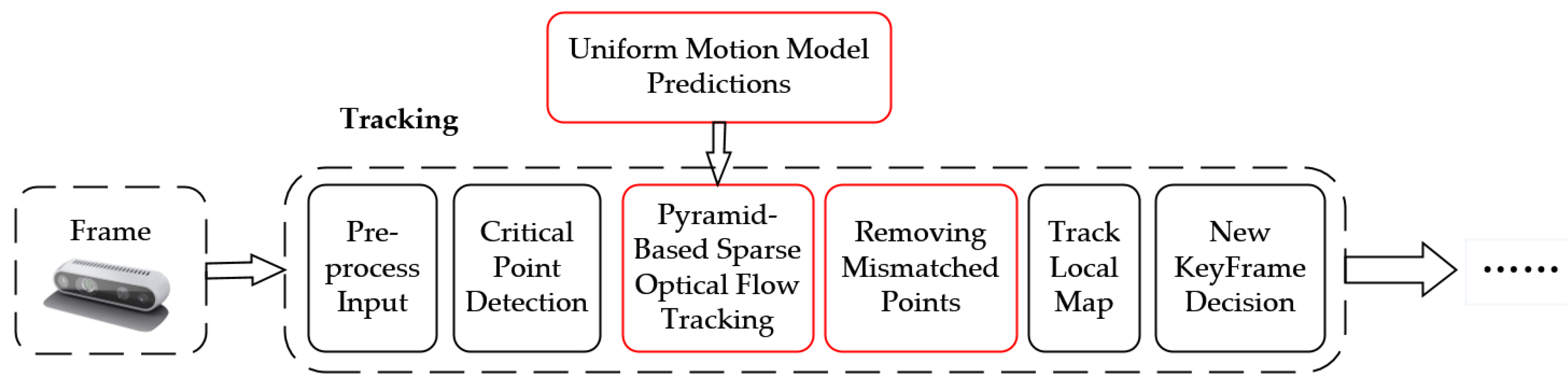
2.1. Algorithm Framework

As shown in Figure 1, the algorithm in this paper takes an RGB-D frame input. After the preprocess input and key point detection are performed, a robust key point matching relationship between adjacent images is established by combining a uniform motion model with a pyramid-based sparse optical flow tracking algorithm, and then a combined strategy of removing mismatched points is used for the fast and precise rejection of false match points, local map tracking, and keyframe detection, followed by threads.

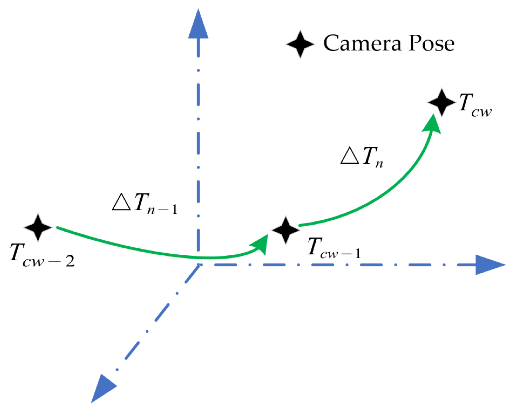
2.2. Prediction of Initial Correspondence of Key Points

When the motion range of the camera is large or it is in a weak texture area, a local minimum is prone to appear with the optical flow method, which leads to the failure of the tracking algorithm. To deal with this problem, a uniform motion model is proposed in this paper, as shown in Figure 2. The position of the key points of the previous image in the current frame is predicted by the uniform motion model, which provides a good initial value for the pyramid-based LK optical flow matching algorithm mentioned in the following section. It can effectively reduce the number of iterations of the optical flow method, thereby improving the robustness and real-time performance of the tracking-matching algorithm.

As shown in Figure 2, define $T_{cw},T_{cw-1},T_{cw-2}\in SE\left(3\right)$ as the poses of the camera in the world coordinate system for the nth, (n − 1)th, (n − 2)th images. Among them, $T_{cw},T_{cw-1}$ are the camera poses of the current and the previous images. Considering that the acquisition frequency of the camera is usually high, as well as the motion amplitude between adjacent image frames is small and continuous, it is supposed that the motion of the camera follows a uniform motion model in a short period, which means the camera motion increment of the current image is the same as that of the previous image. So there is

$$\mathsf{\Delta }{T}_n=\mathsf{\Delta }{T}_{n-1}$$

(1)

where $\mathsf{\Delta }{T}_n$ is the relative pose variation of the camera between the nth image and the (n − 1)th image, and $\mathsf{\Delta }{T}_{n-1}$ is the relative position variation of the camera between the (n − 1)th image and the (n − 2)th image. Given that $T_{cw-1}$ and $T_{cw-2}$ are known, the initial camera position $T_{cw}^{*}$ of the current image can be predicted as follows:

$$T_{cw}^{*}=\mathsf{\Delta }{T}_n{T}_{cw-1}$$

(2)

As shown in Figure 3, when the coordinate $I_{cw-1}\left(x,y\right)$ of a key point in the reference image (previous frame) and the corresponding map point $\left(X,Y,Z\right)$ of the key point in the world coordinate system are given, the camera position of the current frame can be predicted with Formula (2). Project the map point to the image coordinate system of the current frame via the camera model, and the predicted coordinate of the point in the current frame can be obtained as $I_{cw}\left(x^{*},y^{*}\right)$:

$$p^{*}=\frac{1}{Z}K{T}_{cw}^{*}{P}_w$$

(3)

where, $p^{*}={\left[x^{*},y^{*},1\right]}^T$, $P_w={\left[X,Y,Z,1\right]}^T$, Z is the depth value of the key point in the camera coordinate system, and K is the intrinsic matrix of the camera. All the key points in the previous image can be predicted in the current image with Formula (3). Then, the reliable key point matching relationship between the adjacent images is established via a pyramid-based LK optical flow-tracking algorithm. Thus, the problem that the optical flow method easy to drop into local minima is improved, and the robustness and real-time performance of the algorithm are enhanced.

2.3. Pyramid-Based Sparse Optical Flow Tracking Matching

The descriptors of the normal frames cannot be reused in the local optimization and loopback detection threads, which causes a serious waste of computing resources. Therefore, the motion model is combined with the pyramid-based LK optical flow method without calculating the descriptors of normal frames in this paper, and the key points in the reference frame (previous frame) image are tracked to establish a robust key point-matching relationship between the adjacent images.

In LK optical flow, the image can be viewed as a function of time and position, and the function range is the grayscale value of the pixels in the image. Due to the motion of the camera, the position of the same spatial point is different in adjacent images. To estimate the position of this point in the adjacent image, the assumptions of grayscale invariance and neighborhood motion consistency are introduced into the optical flow method. Combined with Taylor expansion, it can be obtained via

$$\left[I_x{I}_y\right]\left[\begin{array}{c}u\\ v\end{array}\right]=-I_t$$

(4)

where, $u$,$v$ are the motion velocities of a pixel on the x-axis and y-axis, respectively, $I_x,I_y$ are the gradient in the x and y direction of the image at that point, and $I_t$ is the change of gray value with time. Because two unknown variables $u$,$v$ are included, the equation cannot be solved. We can use the hypothesis of motion invariance in the optical flow method, select all pixels within the window $n\times n$, and establish $n^2$ equations. Then, the equations can be solved via the least squares method.

Suppose that the pixel coordinates of a key point P in the reference image (previous image) $I_r$ are (x,y), the predicted pixel coordinates of point P in the current image $I_c$ can be calculated as $\left(x_{}^{*},y_{}^{*}\right)$. However, due to the movement of the camera, point P moves to the position $\left(x^{*}+d_x,y^{*}+d_y\right)$ in the current image. The key-point-matching relationship between the adjacent images can be established by solving the motion vector $\left(d_x,d_y\right)$ of this point. Based on the assumptions of the optical flow method, the optical flow calculation problem can be converted to solve $\left(d_x,d_y\right)$ to minimize the change of the pixel gray value in the neighborhood window of the key points in the adjacent image. The grayscale variation function is defined as

$$\delta \left(d_x,d_y\right)={\displaystyle \sum _{x=-w_x}^{w_x}{\displaystyle \sum _{y=-w_y}^{w_y}\left(I_r\left(x,y\right)-I_c\left(x^{*}+d_x,y^{*}+d_y\right)\right)}}$$

(5)

where, $w_x$,$w_y$ are the neighborhood window ranges expanded around key point P. The neighborhood window of point P is $\left(2w_x+1\right)\times \left(2w_y+1\right)$. In this paper, both $w_x$ and $w_y$ are set to 2, and there are a total of 25 pixels in the window.

Therefore, the objective function for solving the motion vector can be defined as

$$\left(d_x,d_y\right)=\underset{d_{x,}{d}_y}{arg\min }{\displaystyle \sum _{i=1}^m{\Vert I_r\left(x_i,y_i\right)-I_c\left(x_i^{*}+d_x,y_i^{*}+d_y\right)\Vert }_{}^2}$$

(6)

where, m represents the number of pixels in the neighborhood window of key points, which is set as m = 25 in this paper. Through the above derivation, it can be seen that the solution of the objective function is a nonlinear optimization problem. The closer the initial value of the optimization is to the optimal value, the easier the algorithm converges. When the camera movement is large, the assumptions of the optical flow method are not valid, which makes the algorithm easy to fall into minimum and fail. To solve this problem, a pyramid structure similar to that used in the ORB feature extraction is introduced. When the motion amplitude of pixels in the original image is large, the motion of these points is still small when observed at the higher levels of the pyramid, so that the algorithm can be applied to the scene where the camera moves rapidly, and accordingly, the robustness and efficiency of the LK optical flow method are improved.

In this paper, the LK optical flow method is used to iteratively solve the motion vectors of key points in the pyramid image. As shown in Figure 4, when calculating the optical flow, it is started from the topmost image of the pyramid, and the predicted value of the key point in the current frame is obtained by the uniform motion model, which is used as the initial value of the top-level iteration to calculate the motion vector of the top-level. Then, the tracking result of the previous layer is used as the iterative initial value of the optical flow of the next layer and the motion vector of the layer is calculated. The process is repeated between the adjacent layers of the pyramid until the lowest layer of the pyramid (the original image) is reached, to obtain the final motion vector and achieve the key point matching between the adjacent images. To evaluate the tracking accuracy of key points and reduce the number of iterations of the optical flow solution, a judging criterion for stopping the iteration of the algorithm is set in this paper, based on the average residual of pixels in the neighborhood window of key points. The average grayscale difference of pixels in the neighborhood window of the corresponding key points between the adjacent images can be expressed via the following equation:

$${\delta }_{ave}=\frac{{\displaystyle \sum _{i=1}^m\Vert I_r\left(x_i,y_i\right)-I_c\left(x_i^{*}+d_x,y_i^{*}+d_y\right)\Vert }}{25}$$

(7)

The termination condition of algorithm iteration is

$${\delta }_{ave}<{\delta }_{\min }\left|\right|N_{iter}>N_{\max }$$

(8)

where ${\delta }_{\min }$ is the minimum value of the average grayscale difference of the pixels in the two neighborhood windows, $N_{iter}$ is the current iteration number of the algorithm, $N_{\max }$ is the maximum number of iterations allowed by the algorithm, and we set ${\delta }_{\min }=0.02,N_{\max }=10$ in the experiment.

As described above, the difference between the VO studied in this paper with the ordinary optical flow method is that an initial value is provided for the pyramid-based LK optical flow tracking algorithm by the uniform motion model, and a termination condition for the algorithm iteration is set, which makes the algorithm to remain good adaptability in dealing with the large camera motion of the camera or the weak texture area. While ensuring the accuracy of the algorithm, the number of iterations is greatly reduced, and the robustness of the algorithm is effectively improved.

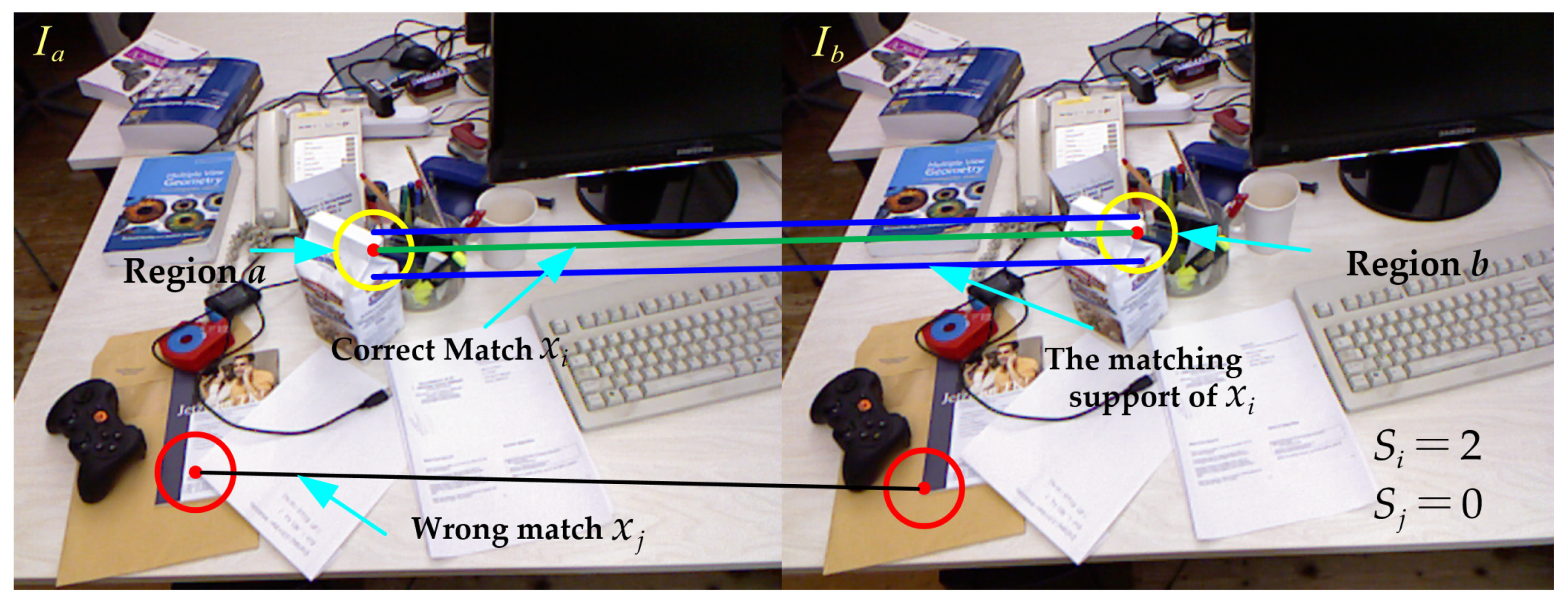
2.4. Strategy for Removing Mismatched Points

By combining the uniform motion model and the pyramid-based LK optical flow method, a robust initial key point matching set can be established between two adjacent images. However, mismatches may still occur. To solve this problem, a combined mismatch point (outer point) elimination algorithm is adopted in this paper to filter out the outer points. The specific process is shown in Figure 5. The main idea is to combine different outlier rejection algorithms to eliminate outer points in turn. This can effectively combine the advantages of different algorithms to improve the speed and accuracy of outlier rejection.

For the matching set of initial key points, the GMS algorithm is used to quickly filter out the external points. Then, RANSAC is used for secondary refinement to obtain the optimal matching set, which provides accurate matching points for the pose estimation of the camera. The advantage of this design is that it combines the fast robustness of the GMS algorithm with the accuracy of the RANSAC algorithm. Before using the RANSAC algorithm to eliminate outliers, most of the outliers in the initial matching set have been quickly eliminated via the GMS algorithm, which provides a matching set with fewer outliers for the RANSAC algorithm, so that the RANSAC algorithm can converge to the correct result faster.

The core idea of the GMS algorithm is that the correct key point matching should satisfy the motion smoothness constraint, which means there are more matching pairs in the neighborhood of the correct matching point for support, while the wrong matching point does not have this property. As shown in Figure 6, suppose there are $\left\{M,N\right\}$ key points in two adjacent images $\left\{I_a,I_b\right\}$ and the initial key point matching set is $X=\left\{x_1,x_2,\cdots ,x_i,\cdots x_N\right\}$, where $x_i$ represents the matching pair i, and the neighborhood of this matching pair is defined as $\left\{a,b\right\}$. The neighborhood of the correct matching point is in the yellow circle, and the neighborhood of the false matching point is in the red circle. The support quantity of the matching pair in the neighborhood of the correct matching $x_i$ is $S_i=2$, while the support quantity of the matching pair in the neighborhood of the incorrect matching $x_j$ is $S_j=0$. Outliers can be identified and filtered out by the support of matching pairs in the neighborhood.

To improve the real-time performance of the algorithm, the GMS algorithm divides the image into $G\times G$ non-overlapping grids and counts the support of matching pairs within K neighborhoods of the matching points to calculate the synthesis score $S_i$. The calculation of the neighborhood matching pair can be accelerated by the gridding images, which effectively reduces the complexity of the algorithm. The value $S_i$ can be calculated via the following formula:

$$S_i={\displaystyle \sum _{k=1}^{k=9}\left|x_{a^k{b}^k}\right|}-1$$

(9)

where $x_{a^k{b}^k}$ is the corresponding matching subset in the neighborhood $x_i$, k is the number of neighborhood grids. The larger the value of $S_i$ the higher the probability that matching is correct. Since the matching relationships of each key point are independent, $S_i$ can be treated as an approximate binomial distribution.

$$S_i~\{\begin{array}{l}B\left(kn,p_t\right),x_i\mathrm{is} \mathrm{a} \mathrm{true} \mathrm{match}\hfill \\ B\left(kn,p_f\right),x_i\mathrm{is} \mathrm{a} \mathrm{false} \mathrm{match}\hfill \end{array}$$

(10)

The mean m and standard deviation s of a binomial distribution $S_i$ can be expressed via the following equation:

$$\{\begin{array}{l}{m}_t=Kn{p}_t,s_t=\sqrt{Knt\left(1-pt\right)},x_i\mathrm{is} a \mathrm{true} \mathrm{match}\hfill \\ m_f=Kn{p}_t,s_f=\sqrt{Knt\left(1-pt\right)},x_i\mathrm{is} a \mathrm{false} \mathrm{match}\hfill \end{array}$$

(11)

The discrimination between true matching and false matching is defined as p:

$$p=\frac{m_t-m_f}{s_t+s_f}=\frac{kn{p}_t-kn{p}_f}{\sqrt{kn{p}_t\left(1-p_t\right)+kn{p}_f\left(1-p_f\right)}}\propto \sqrt{kn}$$

(12)

When the value p is larger, the difference between true and false matching is greater, and the ability of the model to distinguish true and false matching is stronger. The outlier rejection threshold is set to ${\tau }_i=\alpha \sqrt{n_i}$, where $\alpha$ is a weight factor and $n_i$ is the average matching number of the key points in 9 neighborhood grids. It has been determined experimentally that better results can be obtained when $\alpha =6$. If $S_i>{\tau }_i$, $x_i$ is considered a correct matching; otherwise, it is an incorrect matching and will be removed. Thus, the matching point set after preliminary screening is obtained. The RANSAC algorithm is used to purify the key point matching set after the preliminary screening. The steps are as follows:

(1)

Randomly select eight pairs of matching points from the matching points after the preliminary screening, and use the eight-point algorithm to solve the fundamental matrix F.

(2)

Calculate the Simpson distance d between the remaining matching point pairs according to Formula (13). If $d<\tau$, it is considered that the matching point pair is an internal point. Otherwise, it is considered an external point. Record the number of internal points at this time.

$$d\left(x_n{}_1,x_n{}_2\right)=\frac{{\left(x_n{}_2^{T}F{x}_n{}_1\right)}^2}{{\left(F{x}_n{}_1\right)}_x^2+{\left(F{x}_n{}_1\right)}_y^2+{\left(x_{n2}^{T}F\right)}_x^2+{\left(x_n{}_2^{T}F\right)}_y^2}$$

(13)

(3)

Repeat the above steps. If the number of iterations reaches the set threshold or the ratio of the number of internal points to all matching points reaches the set threshold during an iteration, stop the iteration. Then, select the fundamental matrix with the highest confidence and eliminate all matching points that do not meet the condition of $d<\tau$ in the matching point set after preliminary screening, to obtain the optimal matching point set.

A robust initial rough matching relationship of key points between the adjacent images can be established via the pyramid optical flow tracking matching algorithm based on the motion model, and then use the combined mismatch elimination algorithm to eliminate the possible external points to ensure the accuracy of the camera pose solved by the system, providing a strong guarantee for the accurate positioning of the robot and the construction of an accurate environmental map.

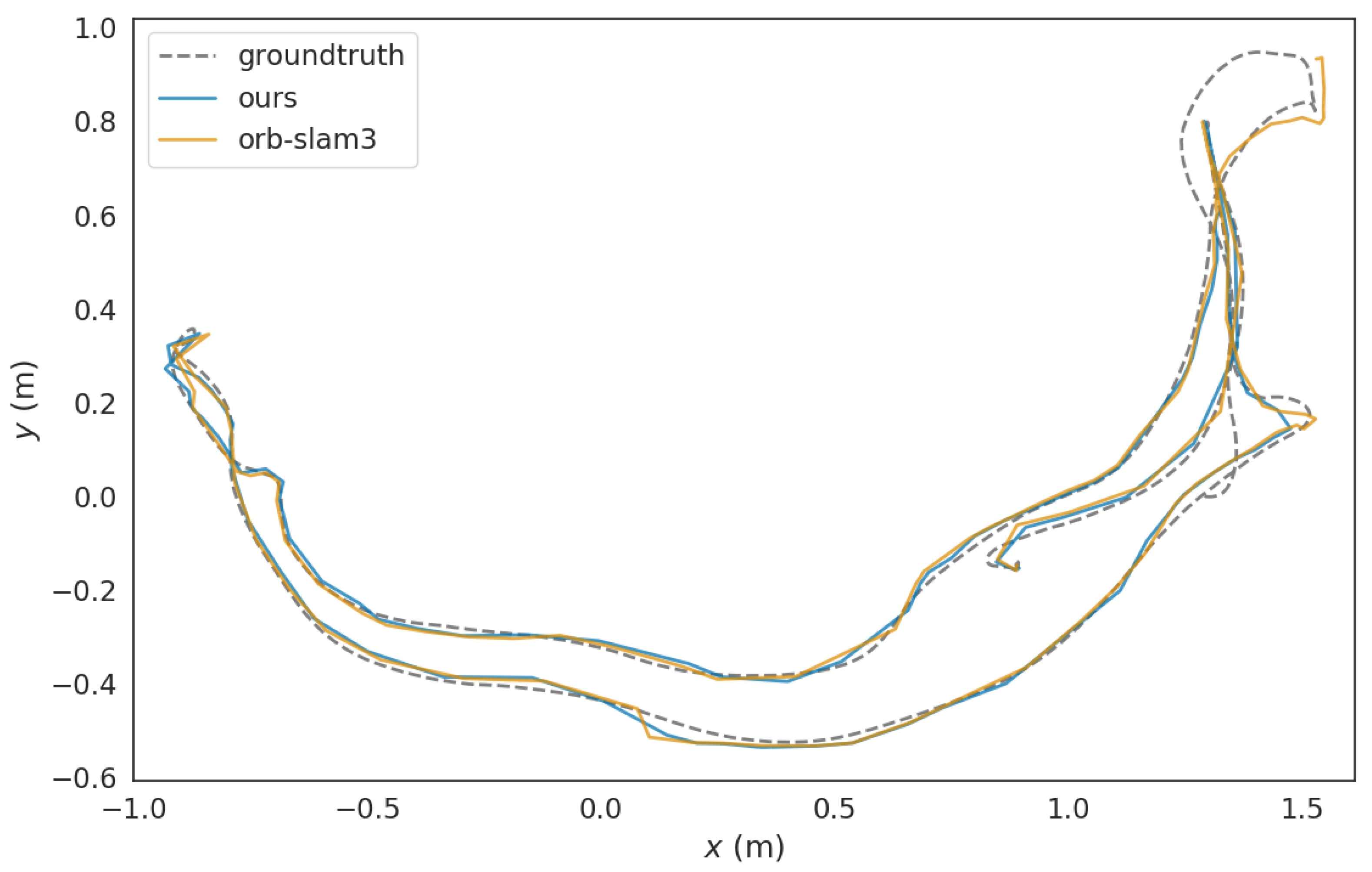
3. Experiment and Analysis

In this section, the proposed lightweight VO based on optical flow tracking is quantitatively evaluated from the perspectives of positioning accuracy and efficiency, and its accuracy and running speed are analyzed. All experiments were run on Ubuntu 18.04 LTS using an Inter(R) Core(TM) i5-6300 @2.30 GHz CPU and 8 GB RAM. To verify the effectiveness of the system in different indoor scenarios, four representative sequences are selected from both the TUM dataset [32] and the ICL-NUIM dataset [33] for testing purposes.

To minimize the influence of the random errors of the system on the experimental results, take all data with the average value of 20 experiments.

Table 1. Comparison of RMSE.

Sequence	RMSE (m)		Improvement
	Ours	ORB-SLAM3
fr1-xyz	0.012	0.011	-
fr1-room	0.042	0.045	6.67%
fr1-desk2	0.023	0.025	8.00%
fr2-large	0.12	0.107	-
fr2-rpy	0.003	0.003	-
fr2-person	0.005	0.006	16.67%
fr3-office	0.011	0.013	15.38%
fr3-notx-near	0.018	0.021	14.29%
fr3-tx-near	0.012	0.01	-
office2	0.017	0.02	15.00%
office3	0.066	0.06	-
living2	0.021	0.019	-
living3	0.012	0.013	7.69%

and

Table 2. Comparison of per frame average runtime.

Sequence	Average Time Consumption (s)		Improvement
	Ours	ORB-SLAM3
fr1-xyz	0.024	0.029	17.24%
fr1-room	0.016	0.021	23.81%
fr1-desk2	0.013	0.019	31.58%
fr2-large	0.015	0.022	31.82%
fr2-rpy	0.022	0.027	18.52%
fr2-person	0.024	0.034	29.41%
fr3-office	0.014	0.019	26.32%
fr3-notx-near	0.01	0.013	23.08%
fr3-tx-near	0.022	0.029	24.14%
office2	0.015	0.021	28.57%
office3	0.017	0.023	26.09%
living2	0.015	0.022	31.82%
living3	0.018	0.027	33.33%

show the positioning accuracy of the two systems under 13 different sequences and the per-frame average runtime. RMSE represents the root mean square error of the absolute trajectory error and the average runtime represents the time required to process each image.

From the analysis of Table 1, it can be seen that both the system proposed in this paper and the ORB-SLAM3 system have high precision and robustness in all 13 sequences. However, the system proposed in this paper performs slightly better in 7 of the sequences, in which positioning accuracy is close to and slightly improved compared with the ORB-SLAM3 system; the reason for the poor accuracy in the other six sequences is that the image texture in the sequence is clear and rich in key points, motion model prediction error is larger than the original tracking error. From the analysis of Table 2, in average runtime, the system proposed in this paper is significantly better than ORB-SLAM3 in all 13 sequences. The improvement is most evident in the fr1-room sequence which achieves 34.8%. The reason is that the key point-matching relationship between adjacent images is established in the proposed system without calculating descriptors, which results in a significant improvement in efficiency and real-time performance.

Since the sequences, fr1-desk2 and office2, are relatively stable and have clear trajectories, they were selected for comparison. Via the EVO toolkit [34], the parameters in the absolute pose error (APE) and relative pose error (RPE) of the two system trajectories are quantitatively analyzed for further testing of the system performance. At the same time, to observe the differences between the trajectories more clearly, the original trajectory is projected onto a two-dimensional plane for comparison.

Figure 7 shows the comparison projected onto the x-o-y plane between the ground truth and the trajectories generated by the proposed system and the ORB-SLAM3 system under the fr1-desk2 sequence. The dashed line represents the ground truth of the dataset, while the blue and orange curves represent the trajectories of the proposed system and the ORB-SLAM3 system. Both systems passed the test under this sequence, indicating that both systems have good robustness. However, the trajectory of the system proposed in this paper is closer to the ground truth in some local areas.

Figure 8 shows the APE comparison between the two systems under the fr1-desk2 sequence. The histogram compares the error parameters of the APE in the two systems, and the box diagram shows the fluctuation of the data. The histogram analysis shows that the supposed system in this paper outperforms the ORB-SLAM3 system in five of the APE error parameters, including the RMSE, minimum error (Min), median error (Median), mean error (Mean), and maximum error (Max). However, it is slightly inferior to the ORB-SLAM3 system in the standard error (Std), but the difference is relatively small. According to the box plot analysis, the data fluctuation of the proposed system is slightly smaller than that of the ORB-SLAM3 system. It shows that the positioning accuracies of the two systems are better under this sequence, and the differences among the various parameters in APE are small. However, on the whole, the positioning accuracy and stability of the proposed system in this paper are slightly better than that of ORB-SLAM3, and RMSE for translation is 0.021, which meets the requirements of positioning and map construction.

Figure 9 shows the RPE comparison between the two systems under the fr1-desk2 sequence. Through the detailed analysis of the figure, it can be seen that all the RPE data of the proposed system are better than those of the ORB-SLAM3 system. So it can be concluded that the comprehensive performance of the proposed system is better than that of the ORB-SLAM3 system under this sequence.

Figure 10 shows the comparison projected onto the x-o-z plane between the ground truth and the trajectories generated via the proposed system and the ORB-SLAM3 system under the office3 sequence. It can be seen from the figure that the trajectories generated by the two systems are consistent with the ground truth provided by the dataset, which indicates that both systems have achieved good performance under this sequence. However, as indicated by the red squares in the figure, the ORB-SLAM3 system has a large error. The reason is that the texture of the region is low and the key points are not rich enough, resulting in poor feature matching of the system. Because the proposed system tracks and matches the key points by the pyramid-based sparse optical flow method, more key points can be tracked in the area with lower texture, improving the accuracy and robustness of the system.

Figure 11 and Figure 12 show the comparisons of the APE and RPE of the two systems under the sequence, office2. Through specific analysis, we know that all the data of APE and RPE of the proposed system are better than those of the ORB-SLAM3 system, and the data fluctuation range is smaller.

Figure 13 shows the comparison projected onto the two-dimensional plane between the ground truth and the trajectories generated by the proposed system and the ORB-SLAM3 system under the other sequences. Among them, it can be seen that the VO in this paper is closer to the ground truth in the local trajectory from the (a) sequence, and the (b, d, e) sequence shows that both algorithms are close to the ground truth. Due to the dynamic objects present in the (c) sequence, both two algorithms produce a drift when they estimate the camera pose in the part of the image stream where dynamic objects are present, which shows a lack of ability to deal with dynamic objects.

4. Conclusions

In this paper, a lightweight, front-end VO based on optical flow tracking has been proposed to solve the problem that the visual SLAM system based on feature points has good robustness but poor real-time performance. Without calculating the descriptors, the reliable matching relationship of key points between the adjacent images has been established by combining the uniform motion model with the pyramid-based sparse optical flow method. GMS and RANSAC algorithms were used to filter out the outliers in turn. To verify the effectiveness of the proposed algorithm in different environments, experiments have been carried out in two datasets of TUM and ICL-NUIM and compared with ORB-SLAM3. According to the experimental results, although the RMSE of the proposed method is not much different from ORB-SLAM3, the proposed method can effectively improve the efficiency up to 27.3% on average, which will greatly reduce the computation quantity of the system.

In the future, we will improve and refine our work further in the following aspects: First, according to our experimental results, using the same motion prediction model for different scenarios may lead to accuracy degradation. Thus, we will consider experimenting with different motion prediction models in the same scene to research the adaptability of the motion model to the scene. Second, in the experimental part of this paper, only comparative tests with ORB-SLAM3 have been performed at present; we will look for other representative methods to compare and contrast to increase the validity of the paper. Finally, the work presented in this paper does not involve the lower-layer control and estimation of robots yet. Thus, the adaptability of the improved algorithm to various types of lower-layer control is also a very valuable research direction.

References

1. Leonard, J.J.; Durrant-Whyte, H.F. Simultaneous Map Building and Localization for an Autonomous Mobile Robot. In Proceedings of the IROS ‘91: IEEE/RSJ International Workshop on Intelligent Robots and Systems’91, Osaka, Japan, 3–5 November 1991; IEEE: Osaka, Japan, 1991; pp. 1442–1447. [Google Scholar]
2. Taketomi, T.; Uchiyama, H.; Ikeda, S. Visual SLAM Algorithms: A Survey from 2010 to 2016. IPSJ Trans. Comput. Vis. Appl. 2017, 9, 16. [Google Scholar] [CrossRef]
3. Li, H.; Zhou, Y.; Dong, Y.; Li, J. Research on Navigation Algorithm of Ros Robot Based on Laser SLAM. World Sci. Res. J. 2022, 8, 581–584. [Google Scholar]
4. Chen, Z.; Qi, Y.; Zhong, S.; Feng, D.; Chen, Q.; Chen, H. SCL-SLAM: A Scan Context-Enabled LiDAR SLAM Using Factor Graph-Based Optimization. In Proceedings of the IEEE International Conference on Unmanned Systems (ICUS), Guangzhou, China, 28–30 October 2022; pp. 1264–1269. [Google Scholar]
5. Shan, T.; Englot, B.; Meyers, D.; Wang, W.; Ratti, C.; Rus, D. LIO-SAM: Tightly-Coupled Lidar Inertial Odometry via Smoothing and Mapping. In Proceedings of the IEEE/RSJ International Conference on Intelligent Robots and Systems (IROS), Las Vegas, NV, USA, 25–29 October 2020. [Google Scholar]
6. Zhou, H.; Yao, Z.; Lu, M. UWB/Lidar Coordinate Matching Method with Anti-Degeneration Capability. IEEE Sens. J. 2021, 21, 3344–3352. [Google Scholar] [CrossRef]
7. Camurri, M.; Ramezani, M.; Nobili, S.; Fallon, M. Pronto: A Multi-Sensor State Estimator for Legged Robots in Real-World Scenarios. Front. Robot. AI 2020, 7, 68. [Google Scholar] [CrossRef] [PubMed]
8. Lin, J.; Zheng, C.; Xu, W.; Zhang, F. R2LIVE: A Robust, Real-Time, LiDAR-Inertial-Visual Tightly-Coupled State Estimator and Mapping. IEEE Robot. Autom. Lett. 2021, 6, 7469–7476. [Google Scholar] [CrossRef]
9. Lin, J.; Zhang, F. R3LIVE: A Robust, Real-Time, RGB-Colored, LiDAR-Inertial-Visual Tightly-Coupled State Estimation and Mapping Package. In Proceedings of the International Conference on Robotics and Automation (ICRA), Philadelphia, PA, USA, 23–27 May 2021. [Google Scholar]
10. Meng, Z.; Xia, X.; Xu, R.; Liu, W.; Ma, J. HYDRO-3D: Hybrid Object Detection and Tracking for Cooperative Perception Using 3D LiDAR. IEEE Trans. Intell. Veh. 2023, 8, 1–13. [Google Scholar] [CrossRef]
11. Kim, M.; Zhou, M.; Lee, S.; Lee, H. Development of an Autonomous Mobile Robot in the Outdoor Environments with a Comparative Survey of LiDAR SLAM. In Proceedings of the 22nd International Conference on Control, Automation and Systems (ICCAS), Busan, Republic of Korea, 27 November–1 December 2022; pp. 1990–1995. [Google Scholar]
12. Yang, S.; Zhao, C.; Wu, Z.; Wang, Y.; Wang, G.; Li, D. Visual SLAM Based on Semantic Segmentation and Geometric Constraints for Dynamic Indoor Environments. IEEE Access 2022, 10, 69636–69649. [Google Scholar] [CrossRef]
13. Jie, L.; Jin, Z.; Wang, J.; Zhang, L.; Tan, X. A SLAM System with Direct Velocity Estimation for Mechanical and Solid-State LiDARs. Remote Sens. 2022, 14, 1741. [Google Scholar] [CrossRef]
14. Davison, A.J.; Reid, I.D.; Molton, N.D.; Stasse, O. MonoSLAM: Real-Time Single Camera SLAM. IEEE Trans. Pattern Anal. Mach. Intell. 2007, 29, 1052–1067. [Google Scholar] [CrossRef] [PubMed]
15. Klein, G.; Murray, D. Parallel Tracking and Mapping for Small AR Workspaces. In Proceedings of the 6th IEEE and ACM International Symposium on Mixed and Augmented Reality, Washington, DC, USA, 13–16 November 2007; pp. 225–234. [Google Scholar]
16. Mur-Artal, R.; Montiel, J.M.M.; Tardós, J.D. ORB-SLAM: A Versatile and Accurate Monocular SLAM System. IEEE Trans. Robot. 2015, 31, 1147–1163. [Google Scholar] [CrossRef]
17. Rublee, E.; Rabaud, V.; Konolige, K.; Bradski, G. ORB: An Efficient Alternative to SIFT or SURF. In Proceedings of the International Conference on Computer Vision, Barcelona, Spain, 6–13 November 2011; pp. 2564–2571. [Google Scholar]
18. Mur-Artal, R.; Tardós, J.D. ORB-SLAM2: An Open-Source SLAM System for Monocular, Stereo, and RGB-D Cameras. IEEE Trans. Robot. 2017, 33, 1255–1262. [Google Scholar] [CrossRef]
19. Campos, C.; Elvira, R.; Rodríguez, J.J.G.; Montiel, J.M.M.; Tardós, J.D. ORB-SLAM3: An Accurate Open-Source Library for Visual, Visual–Inertial, and Multimap SLAM. IEEE Trans. Robot. 2021, 37, 1874–1890. [Google Scholar] [CrossRef]
20. Newcombe, R.A.; Lovegrove, S.J.; Davison, A.J. DTAM: Dense Tracking and Mapping in Real-Time. In Proceedings of the International Conference on Computer Vision, Barcelona, Spain, 6–13 November 2011; pp. 2320–2327. [Google Scholar]
21. Engel, J.; Schöps, T.; Cremers, D. LSD-SLAM: Large-Scale Direct Monocular SLAM. In Proceedings of the Computer Vision—ECCV 2014: 13th European Conference, Zurich, Switzerland, 6–12 September 2014; Fleet, D., Pajdla, T., Schiele, B., Tuytelaars, T., Eds.; Lecture Notes in Computer Science. Springer International Publishing: Cham, Switzerland, 2014; pp. 834–849. [Google Scholar]
22. Forster, C.; Pizzoli, M.; Scaramuzza, D. SVO: Fast Semi-Direct Monocular Visual Odometry. In Proceedings of the IEEE International Conference on Robotics and Automation (ICRA), Hong Kong, China, 31 May–5 June 2014; pp. 15–22. [Google Scholar]
23. Engel, J.; Koltun, V.; Cremers, D. Direct Sparse Odometry. IEEE Trans. Pattern Anal. Mach. Intell. 2018, 40, 611–625. [Google Scholar] [CrossRef] [PubMed]
24. Qin, T.; Li, P.; Shen, S. VINS-Mono: A Robust and Versatile Monocular Visual-Inertial State Estimator. IEEE Trans. Robot. 2018, 34, 1004–1020. [Google Scholar] [CrossRef]
25. Zhang, H.; Huo, J.; Sun, W.; Xue, M.; Zhou, J. A Static Feature Point Extraction Algorithm for Visual-Inertial SLAM. In Proceedings of the China Automation Congress (CAC), Xiamen, China, 25–27 November 2022; pp. 987–992. [Google Scholar]
26. Engel, J.; Stückler, J.; Cremers, D. Large-Scale Direct SLAM with Stereo Cameras. In Proceedings of the IEEE/RSJ International Conference on Intelligent Robots and Systems (IROS), Hamburg, Germany, 28 September–3 October 2015; pp. 1935–1942. [Google Scholar]
27. Khairuddin, A.R.; Talib, M.S.; Haron, H. Review on Simultaneous Localization and Mapping (SLAM). In Proceedings of the IEEE International Conference on Control System, Computing and Engineering (ICCSCE), Penang, Malaysia, 27–29 November 2015; pp. 85–90. [Google Scholar]
28. Guo, G.; Dai, Z.; Dai, Y. Real-Time Stereo Visual Odometry Based on an Improved KLT Method. Appl. Sci. 2022, 12, 12124. [Google Scholar] [CrossRef]
29. De Palezieux, N.; Nageli, T.; Hilliges, O. Duo-VIO: Fast, Light-Weight, Stereo Inertial Odometry. In Proceedings of the IEEE/RSJ International Conference on Intelligent Robots and Systems (IROS), Daejeon, Republic of Korea, 9–14 October 2016; pp. 2237–2242. [Google Scholar]
30. Bian, J.-W.; Lin, W.-Y.; Liu, Y.; Zhang, L.; Yeung, S.-K.; Cheng, M.-M.; Reid, I. GMS: Grid-Based Motion Statistics for Fast, Ultra-Robust Feature Correspondence. Int. J. Comput. Vis. 2020, 128, 1580–1593. [Google Scholar] [CrossRef]
31. Fischler, M.A.; Bolles, R.C. Random Sample Consensus: A Paradigm for Model Fitting with Applications to Image Analysis and Automated Cartography. Commun. ACM 1981, 24, 381–395. [Google Scholar] [CrossRef]
32. Sturm, J.; Engelhard, N.; Endres, F.; Burgard, W.; Cremers, D. A Benchmark for the Evaluation of RGB-D SLAM Systems. In Proceedings of the IEEE/RSJ International Conference on Intelligent Robots and Systems, Loulé, Portugal, 7–12 October 2012; pp. 573–580. [Google Scholar]
33. Handa, A.; Whelan, T.; McDonald, J.; Davison, A.J. A Benchmark for RGB-D Visual Odometry, 3D Reconstruction and SLAM. In Proceedings of the IEEE International Conference on Robotics and Automation (ICRA), Hong Kong, China, 31 May–5 June 2014; pp. 1524–1531. [Google Scholar]
34. Grupp, M. Evo: Python Package for the Evaluation of Odometry and Slam. Available online: https://github.com/MichaelGrupp/evo (accessed on 14 October 2017).
Figure 1. The framework of algorithm.
Applsci 13 11322 g001
Figure 2. Uniform Motion Model.
Applsci 13 11322 g002
Figure 3. Prediction of key point correspondence.
Applsci 13 11322 g003
Figure 4. Key point motion vector solution based on the pyramid.
Applsci 13 11322 g004
Figure 5. Combined mismatch point elimination algorithm.
Applsci 13 11322 g005
Figure 6. GMS algorithm diagram.
Applsci 13 11322 g006
Figure 7. The trajectory position comparison diagram of fr1-desk2 sequence.
Applsci 13 11322 g007
Figure 8. Comparison of APE of sequence fr1-desk2. (a) Histogram; (b) box diagram.
Applsci 13 11322 g008
Figure 9. Comparison of RPE of sequence fr1-desk2. (a) Histogram; (b) box diagram.
Applsci 13 11322 g009
Figure 10. The trajectory position comparison diagram of office2 sequence.
Applsci 13 11322 g010
Figure 11. Comparison of APE of sequence office2. (a) Histogram. (b) Box diagram.
Applsci 13 11322 g011
Figure 12. Comparison of RPE of sequence office2. (a) Histogram. (b) Box diagram.
Applsci 13 11322 g012
Figure 13. The trajectory position comparison diagram of the TUM dataset and the ICL-NUIM dataset. (a) fr1-room sequence; (b) fr3-office sequence; (c) fr2-person sequence; (d) fr2-large sequence; (e) living3 sequence.
Applsci 13 11322 g013aApplsci 13 11322 g013b