A Real-Time Simulator for Navigation in GNSS-Denied Environments of UAV Swarms

Featured Application

The findings presented herein can be directly applied for the development of navigation algorithms in gnss-denied environments.

Abstract

Accurate localization is the foundation of unmanned aerial vehicle (UAV) swarm applications in the global navigation satellite system (GNSS)-denied environment. However, the implementation of UAV formation in the real world is costly and time-consuming, which leads to difficulties in developing navigation algorithms. A real-time simulator for navigation in GNSS-denied environments is proposed, which includes world, model, controller, scene matching navigation (SMN), relative navigation and formation controller modules. Each module can be modified, which means that users can test their own algorithms. A novel inertial-aided SMN (ISMN) algorithm is developed and a relative navigation method that does not rely on inter communication is proposed. ISMN and relative navigation based on a camera and ultrawideband (UWB) are tested on the platform. Based on the developed simulation system, the navigation algorithms can be verified easily, which can reduce the time and personnel requirements during flight testing.

1. Introduction

Advances in science and technology in the past decade have brought increased interest towards the development of autonomous UAVs. Swarms are common in nature, such as fish schools, ants and honeybee swarms. The study of UAV swarms based on this biologically inspired concept has become an important trend in UAV development [1,2]. This makes autonomous UAVs a very promising technology for activities such as geological mapping, surveillance, resource gathering and rescue missions, among others. Maintaining, changing and reconstructing formation control is necessary for UAV swarm missions. A fundamental component of UAV swarm missions is a navigation system capable of providing navigation and relative positioning. Currently, most UAV formation controls are based on integrated navigation systems (INS), which include an inertial measurement unit (IMU) and a GNSS receiver. The IMU can accurately estimate the attitude and position of the UAV over a short period of time. However, due to random drift errors in inertial devices, the pose error accumulates over time. A GNSS such as the global positioning system (GPS) is more accurate over longer periods of time. Therefore, an IMU and GNSS are usually combined through extended Kalman filters (EKF) or unscented Kalman filters (UKF) to achieve high-precision pose information over a long time. Generally, UAV swarms can achieve high-precision relative positioning by sharing their locations through internetworking. However, in constantly evolving, high-intensity adversarial environments, relying solely on a GNSS to establish reliable spatial position and velocity measurements relative to geographic coordinate systems has become difficult [3]. With the development of the GNSS, the competition and control over the GNSS and its operating environment are becoming increasingly fierce. Currently, countermeasures such as interference, deception and attacks against GNSS signals and systems are emerging one after another, and the operating environment of satellite navigation systems is gradually deteriorating. The potential threats to the GNSS system mainly include the following: (1) directly killing or interfering with navigation satellites through anti-satellite weapons; (2) the use of radio interference, information security attacks and other means to target ground operation and control stations and other facilities, which makes it difficult for these ground operation and control facilities to function properly, resulting in the inability of the entire navigation system to function properly; (3) using various methods such as suppression interference and deception to directly interfere with the navigation terminal, making it unable to output or mistakenly output navigation information, thereby interfering with the normal use of the navigation system. On the other hand, GNSS signals are affected when passing through environmental objects such as trees, buildings and rocks. These obstacles can cause signal reflection, scattering, refraction, etc., resulting in longer signal propagation paths, weakened signal strengths, phase delays, etc. These impacts can lead to a decrease in the reception quality of GNSS signals, thereby affecting the accuracy of position calculation [4]. Therefore, navigation methods that do not rely on communication under GNSS-denied environments have become increasingly important for UAV swarm applications. Due to the complexity of outdoor environments, UAV formation flying requires a large number of personnel, which leads to high development costs and large time requirements for navigation algorithms. Currently, open-source simulation systems such as Promethues [5], Xtdrone [6,7] and Rflysim [8,9] are more concerned with single control or swarm control, and, in the early stages of developing relative navigation algorithms, it is necessary to verify them in simulation systems to achieve the rapid iteration and validation of the algorithms.

Visual navigation calculates the pose of UAVs relative to ground features to achieve positioning and navigation. Visual navigation has the advantage of minimal environmental impact and high accuracy and has been widely used in GNSS-denied environments [10]. Benefiting from the low cost and high-precision positioning, the SMN system possesses key potential in the GNSS-denied environment [11]. In [12], a novel SMN is proposed, and an optimized factor of the homography matrix is used to reduce the projection errors. In the experiment, the UAV flies at a 150 m height and the flight speed is 12 m/s. The results show that the time consumption for on-matching is 0.6 s and the position error is 4.6 m. In an SMN under GNSS-denied environments, the navigation accuracy is related to the flight altitude. Generally, a navigation error to flight altitude ratio of less than 1% is considered to reflect high precision. Due to factors such as changes in flight altitude and attitude during the flight process, the real-time aerial photos taken by drones exhibit complex geometric distortions, resulting in severe rotation, scaling and even deformation compared to the pre-stored reference images of drones. The inertial information from the IMU is not affected by external factors, which is beneficial. Inertial information can be used to solve the perspective transformation relationship between images [13].

In terms of relative navigation, the work in [14], which investigates onboard visual relative localization in GNSS-denied environments, detects the IDs through black and white colors and achieves localization through the diameter of the circles. Another approach [15] presents a novel onboard relative localization method for swarms of multirotor UAVs. The method uses a new smart sensor called UVDAR, as part of a UVDAR system, which can be used to obtain both the relative position and orientation from a modified camera. Blinking ultraviolet markers are used to identify the ID of the UAV and the orientation. In [16], the author utilizes UWB for peer-to-peer localization.

In this paper, a real-time simulator for navigation in GNSS-denied environments is proposed. The demo video can be found at the following link: https://v.youku.com/v_show/id_XNTk5NDIwMzA3Ng==.html (accessed on 1 October 2023)

The simulator integrates the world environment, sensor physical models, dynamic models of fixed-wing drones and multi-rotor drones, controllers of the drones, a formation controller, an ISMN module, relative navigation based on UWB and a vision module. The contributions of this study are as follows:

(1)

A real-time simulator for navigation in GNSS-denied environments is developed in order to improve the iteration efficiency of navigation algorithms;

(2)

A novel scene matching navigation algorithm called ISMN is proposed; based on the simulator, the ISMN algorithm is validated;

(3)

A relative navigation method that does not rely on inter-communication is proposed.

The remainder of this article is organized as follows. Section 2 describes the architecture of the simulation, which focuses on scene matching navigation and relative navigation. Section 3 describes the sensor model used in the simulation. Section 4 demonstrates the simulation result. In Section 5, the conclusions are summarized.

2. Architecture

As shown in Figure 1, the simulator contains the world, model, controller, ISMN, formation controller and relative navigation modules. In the world module, various environments, such as deserts, grasslands and canyons, can be simulated, which can be used to verify the robustness of the relative navigation. On the other hand, Google Earth containing GPS information is used for the SMN. Sensor models are strongly related to state estimation. In the simulator, a gyroscope, accelerometer, magnetometer, barometer, camera, UWB, etc., can be imported as plugins to supply accurate sensor models for the simulation platform. The controller and formation controller serve for control and swarm motion. Inertia, altitude and images are used for absolute navigation in GNSS-denied environments in the ISMN module. The relative navigation module receives images from cameras and distances from UWB and calculates the relative position for the formation controller.

In the simulation, the flight environment is set through the world module, and the UAV flies in the environment with sensors such as accelerometers, gyroscopes, magnetometers, UWB and cameras and so on. The ISMN module collects the information of the accelerometer, gyroscope, magnetometer and camera and calculates the absolute pose of the UAV. The pose information is sent to the controller module, which can stabilize the UAV through closed-loop control. The relative navigation based on UWB and vision module collects the images of adjacent drones from the camera and the distances of adjacent drones from UWB and calculates the relative position of the UAV. The relative position is sent to the formation controller module, which can implement swarm control.

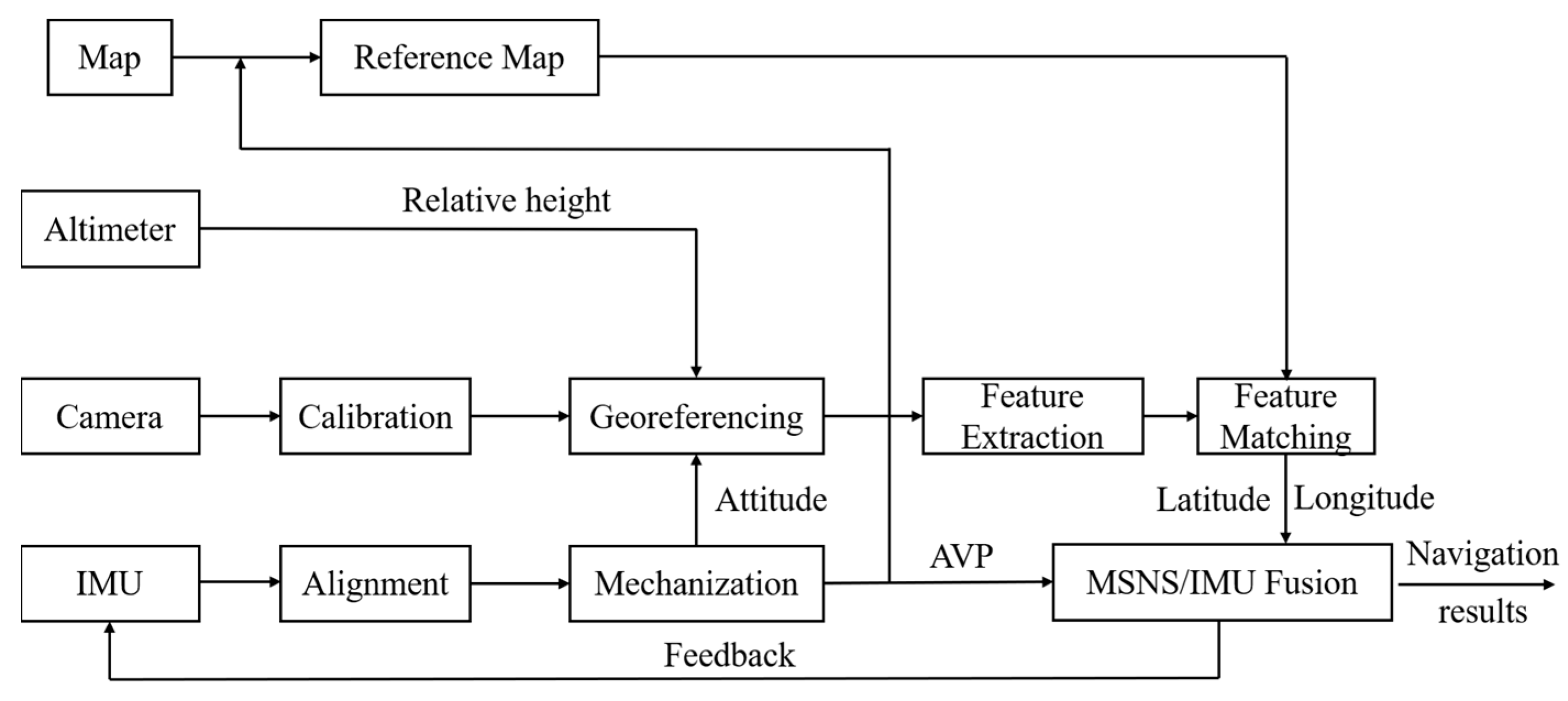
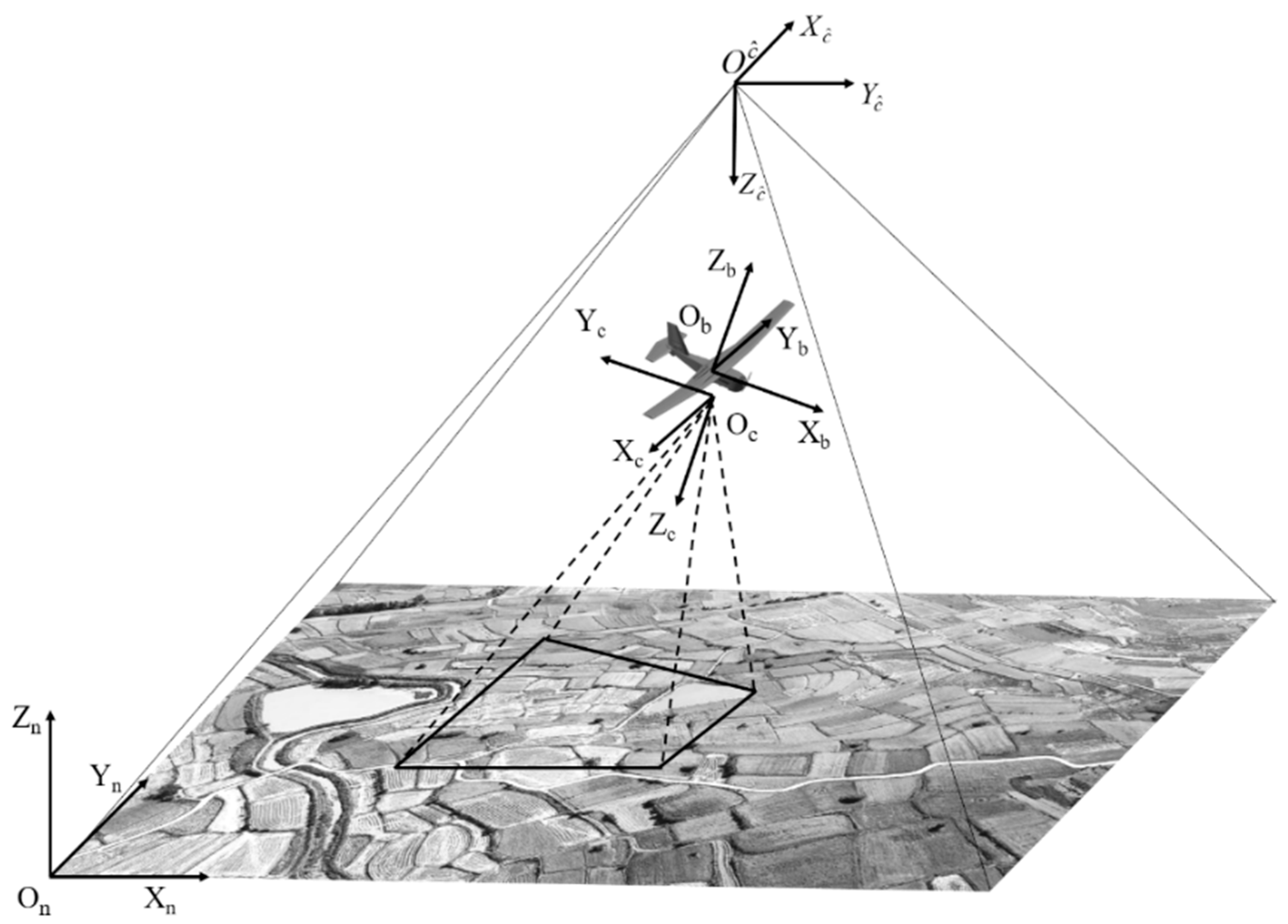
2.1. Inertial-Aided Scene Matching Navigation (ISMN)

SMN is an effective solution for localization in unknown environments when the GNSS is disturbed. We have developed a new localization method that uses local feature points extracted by the Accelerated Robust Feature (SURF) to match the current drone’s captured map image and onboard satellite image, thereby obtaining the position information of the current UAV. In order to improve the efficiency of SMN, the inertial information is obtained for assistance. The ISMN procedure is shown in Figure 2. It uses IMU propagation to determine the scope of the reference satellite map to improve the real-time performance. Considering that the real-time images from the onboard camera and the reference images from the satellite map are not in the same frame, the larger the obliqueness, the higher the probability of mismatching. To solve this problem, we use the attitude from the IMU to correct the real-time input images. This approach enhances the accuracy of image matching in large viewing angles and, consequently, improves the precision of SMN.

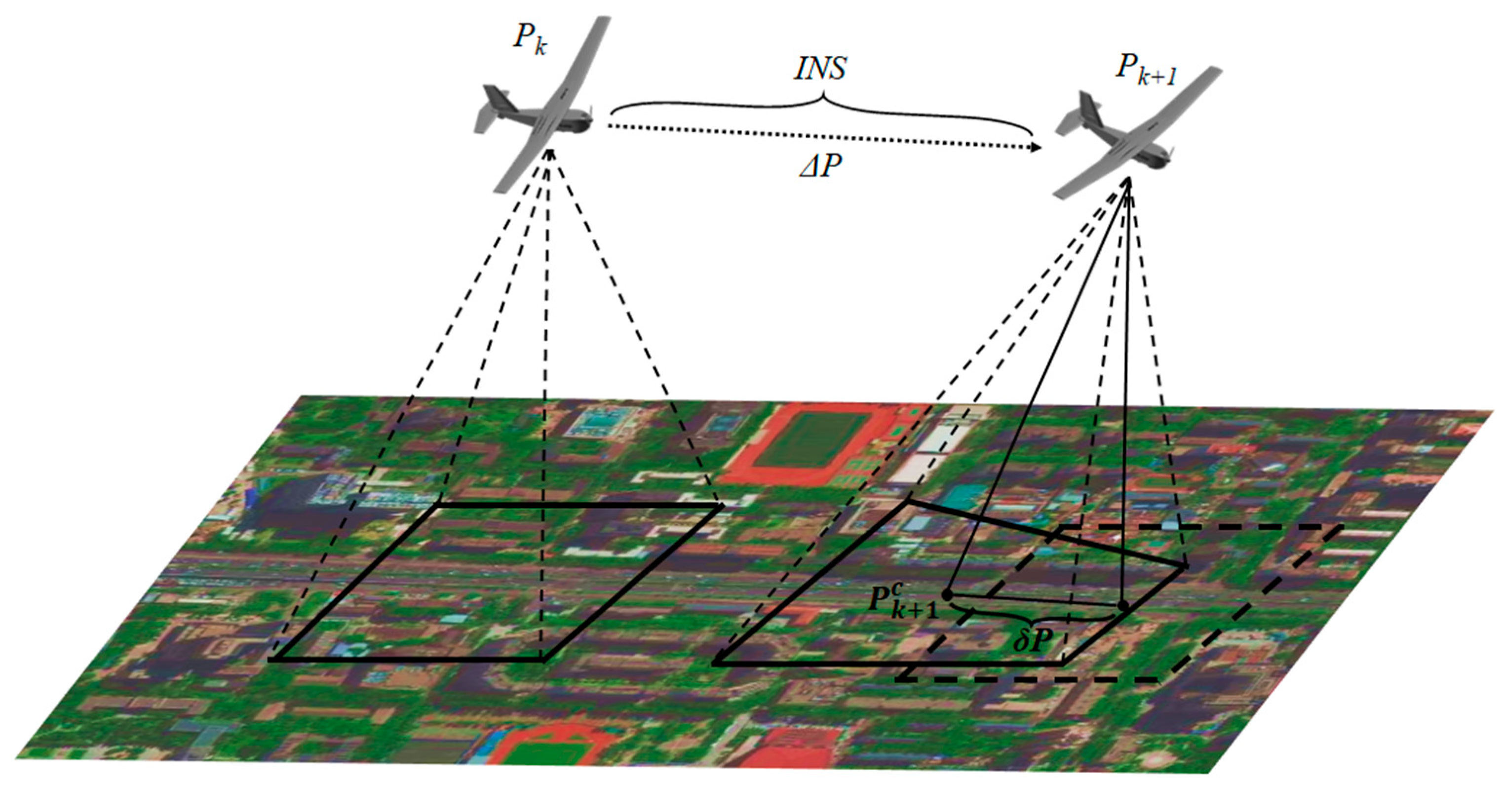
2.1.1. Reference Map from INS Propagation

IMU data are used to narrow the range of satellite images that we need to analyze to perform localization. The propagator is based on the relative acceleration and velocity of the INS model, which is accurate over a short time. As shown in Figure 3, the position of the UAV at time k is $p_k$. After a short time, the position of the UAV at time k + 1 is $p_{k+1}$. The distance at which the UAV flies forward is $\Delta p$, which can be obtained by INS propagation. The deviation $\delta p$ caused by the drone attitude can be obtained through parameters such as the drone flight attitude and altitude. The specific derivation process is as follows.

The velocity update equation with respect to the East, North, Up (ENU) frame in the simplified inertial navigation algorithm is shown in Equation (1).

$${\dot{v}}^n\left(t\right)=C_b^n{f}^b\left(t\right)-\left(2{\omega }_{ie}^n\left(t\right)+{\omega }_{en}^n\left(t\right)\right)\times v^n\left(t\right)+g^n\left(t\right)$$

(1)

$C_b^n$ is the transformation from the body frame (b frame) to the local geographic frame (n frame), $v^n=\left[\begin{array}{ccc}{v}_e& v_n& v_u\end{array}\right]$ represents the velocity in the n frame, $f^b$ is the specific force vector as measured by accelerometers in the b frame, ${\omega }_{ie}^n$ is the rotation rate of the Earth expressed in the n frame, ${\omega }_{en}^n$ is the transport rate, which is only related to the longitude and latitude, and $g^n$ is the local gravitational acceleration vector.

The position update equation in longitude and latitude is shown in Equation (2).

$$\dot{p}=M_{pv}{v}^n$$

(2)

$$p=\left[\begin{array}{c}L\\ \lambda \\ h\end{array}\right]$$

(3)

$$M_{pv}=\left[\begin{array}{ccc}0& 1/R_{Mh}& 0\\ \sec L/R_{Nh}& 0& 0\\ 0& 0& 1\end{array}\right]$$

(4)

$$R_{Mh}=R_M+h, R_{Nh}=R_N+h$$

(5)

$$R_M=\frac{R_N(1-e^2)}{\left(1-e^2{\sin }^{2}L\right)}$$

(6)

$$R_N=\frac{R_e}{{\left(1-e^2{\sin }^{2}L\right)}^{1/2}}$$

(7)

$$e=\sqrt{2f-f^2}$$

(8)

where $L$ represents longitude, $\lambda$ represents latitude, $R_e$ is the Earth’s radius, $e$ is the eccentricity of an ellipsoid and $f\approx 1/298.257$ is the oblateness of the ellipsoid shape.

According to the current longitude, latitude, INS propagation, attitude and height of the drone, we can predict the next feature position in the base map.

The next drone position can be obtained as follows:

$$p_{k+1}=p_k+\Delta p$$

(9)

Concerning the attitude of the drone, the positions of images captured by the camera are derived as

$$p_{k+1}^c=p_{k+1}+\delta p$$

(10)

where

$$\delta p=f\left(\left[\begin{array}{c}\frac{{\rm E}\left(0\right)}{{\rm E}\left(2\right)}\\ \frac{{\rm E}\left(1\right)}{{\rm E}\left(2\right)}\end{array}\right]h\right), {\rm E}=C_b^n{\rm K}, {\rm K}=\left[\begin{array}{c}0\\ 0\\ 1\end{array}\right]$$

$\delta p$ is the drift from obliqueness, $f\left(\right)$ is a transform from the NED coordinate to the WGS-84 coordinate and $h$ is the altitude of the UAV.

According to $p_{k+1}^c$, we can obtain the feature position in the base map, so the number of images that we need to analyze is significantly reduced. We use this method to increase the efficiency of the SMN.

2.1.2. Inertial-Aided Georeference

SMN has a mismatching problem, because the attitude changes during UAV flight will cause differences between the base map and the input images. However, due to the immunity of inertial information to external influences, the inertial information can be utilized to project the real-time image to the reference image coordinates. The matching method aided by inertial information is shown in Figure 4. The attitude of the camera can be estimated from the mechanization results of the IMU. The transformation from the body frame to the navigation frame is $C_b^n$ [17]:

$$C_b^n=\left[\begin{array}{ccc}\cos \gamma \cos \psi & -\cos \theta \sin \psi +\sin \theta \sin \gamma \cos \psi & \sin \theta \sin \psi +\cos \theta \sin \gamma \cos \psi \\ \cos \gamma \sin \psi & \cos \theta \cos \psi +\cos \theta \sin \gamma \sin \psi & -\sin \theta \cos \psi +\cos \theta \sin \gamma \sin \psi \\ -\sin \gamma & \sin \theta \cos \gamma & \cos \theta \cos \gamma \end{array}\right]$$

(11)

where $\psi$, $\theta$ and $\gamma$ denote yaw, pitch and roll, respectively.

The conversion relationship between the camera coordinate system and the IMU coordinate system (body coordinate system) can be expressed as

$$C_c^b=\left[\begin{array}{ccc}\cos {\phi }_y\cos {\phi }_z& -\cos {\phi }_x\sin {\phi }_z+\sin {\phi }_x\sin {\phi }_y\cos {\phi }_z& \sin {\phi }_x\sin \psi +\cos {\phi }_x\sin {\phi }_y\cos {\phi }_z\\ \cos {\phi }_y\sin {\phi }_z& \cos {\phi }_x\cos {\phi }_z+\cos {\phi }_x\sin {\phi }_y\sin {\phi }_z& -\sin {\phi }_x\cos \psi +\cos {\phi }_x\sin {\phi }_y\sin {\phi }_z\\ -\sin {\phi }_y& \sin {\phi }_x\cos {\phi }_y& \cos {\phi }_x\cos {\phi }_y\end{array}\right]$$

(12)

where ${\phi }_x,{\phi }_y,{\phi }_z$ refer to the installation angle between the camera and IMU.

The camera’s optical axis taken from the reference image is almost perpendicular to the ground, $Z_{\widehat{c}}$ is considered to be perpendicular to the ground downwards, $X_{\widehat{c}}$ and $Y_n$ are in the same direction and $Y_{\widehat{c}}$ and $X_n$ are in the same direction, Therefore, there are

$$C_n^{\widehat{c}}\approx \left[\begin{array}{ccc}0& 1& 0\\ 1& 0& 0\\ 0& 0& -1\end{array}\right]$$

(13)

The conversion relationship between the reference maps and real-time maps can be obtained from the above:

$$C_c^{\widehat{c}}=C_n^{\widehat{c}}{C}_b^n{C}_c^b$$

(14)

According to the above conversion relationship and camera parameters, the squint image can be converted to an orthophoto:

$${\widehat{U}}_i=sK{C}_c^{\widehat{c}}{K}^{-1}{U}_i$$

(15)

where $s=\frac{1}{z_c}$, and $z_c$ is the z-direction coordinate component of $U$ in the camera frame.$K$ denotes the internal parameters of the camera, which can be obtained by calibration.

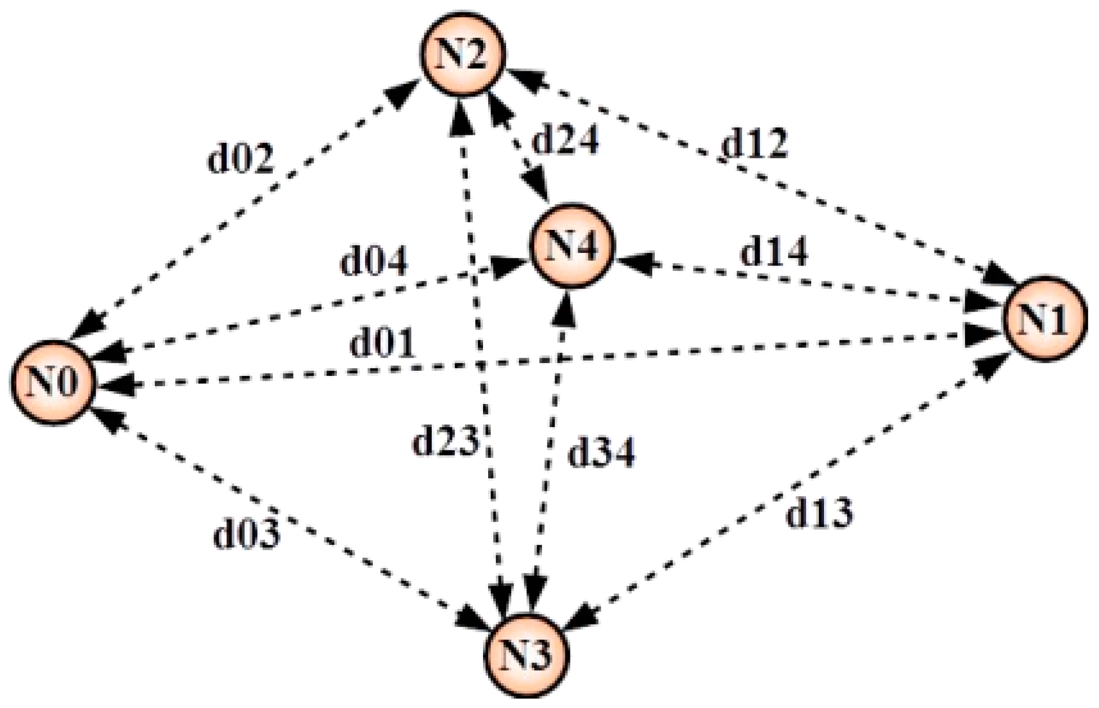
2.2. Relative Navigation Based on Vision and UWB

In this work, we propose the use of local visual information and UWB to perform relative localization. Here, we aim to utilize the onboard sensors including cameras and UWB for relative navigation. In this way, there is no need for inter-communication and localization infrastructure.

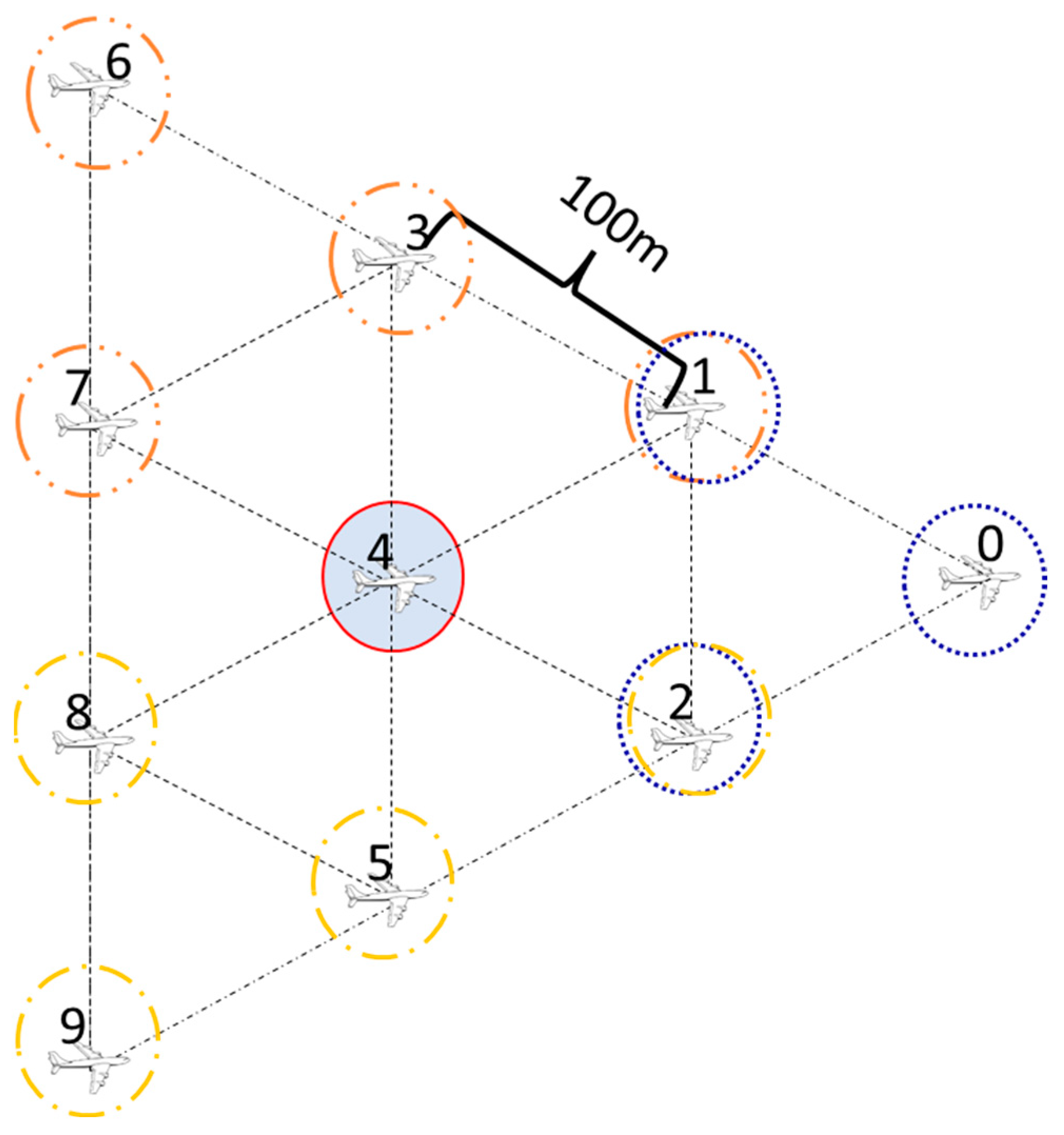
2.2.1. Detection and Tracking of Adjacent UAVs

YOLOv3-tiny [18] is used to detect the adjacent UAVs. YOLOv3-tiny is a lightweight state-of-the-art convolutional neural network (CNN) detector that can work on the on-board computer to provide detection. To utilize the detector to detect adjacent UAVs, an additional training set captured by the camera on the UAV, as well as containing the UAVs, is labeled and fed into the CNN. After training, the CNN is able to detect the UAVs efficiently.

For the tracking of the drone, a KF filter is adopted to predict the trajectory. Moreover, we use the Hungarian algorithm, which is a matching algorithm, to match the detected and predicted result. Blinking LED markers are used to identify unique IDs, preventing all UAVs in the swarm from having a similar appearance.

For the KF filter of the trajectory predicted, the state of the system is

$$x=\left[u,v,\gamma ,h,\dot{u},\dot{v},\dot{\gamma },\dot{h}\right]$$

(16)

where $u$ and $v$ are the center of the object in the image, $\gamma$ is the aspect ratio, $h$ is the altitude and the observation equation can be expressed as

$$z=\left(u,v,\gamma ,h\right)$$

(17)

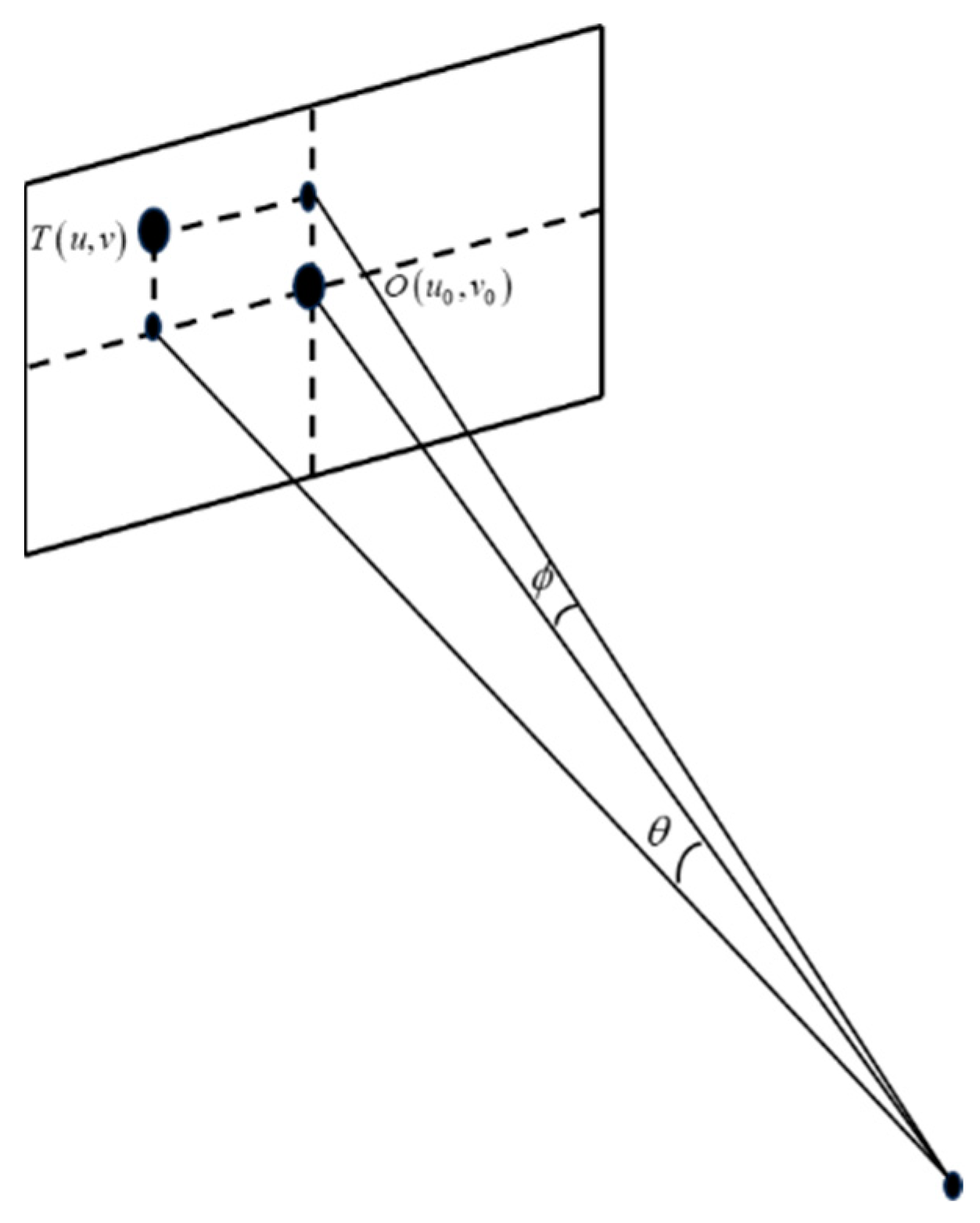
2.2.2. Calculating the Relative Position

The camera imaging plane is shown in Figure 5. $O\left(u_0,v_0\right)$ is the origin located in the image coordinate system. The target’s coordinates in the image coordinate system are denoted by $T\left(u,v\right)$. In the physical coordinate system of the camera, the corresponding coordinate origin is located at $O\left(x_0,y_0\right)$, and the target coordinate system is denoted by $T\left(x,y\right)$. $f$ is the focal length of the camera, and $d_x,d_y$ are the physical sizes of each pixel on the imaging plane along the axis of $x,y$.

$$\{\begin{array}{c}\theta =\arctan \left(\frac{\left(u-u_0\right)\times d_x}{f}\right)\\ \varphi =\arctan \left(\frac{\left(v-v_0\right)\times d_y}{f}\right)\end{array}$$

(18)

where ${\left[\begin{array}{cc}\theta & \varphi \end{array}\right]}^T$ refers to the line-of-sight angle, $\theta$ refers to the line-of-sight azimuth angle and $\varphi$ refers to the line-of-sight elevation angle.

The position among neighboring drones in the swarms can be calculated as

$$u=\rho \left[\begin{array}{c}\sin \left(\varphi \right)\sin \left(\theta \right)\\ \sin \left(\varphi \right)\cos \left(\theta \right)\\ \cos \left(\varphi \right)\end{array}\right]$$

(19)

where $u={\left[\begin{array}{ccc}{u}_x& u_y& u_z\end{array}\right]}^T$.

3. Configuration of Simulator

3.1. Ultrawideband Model

A UWB sensor is a range sensor that can measure the distance between each object within the measurement range. Each UAV is equipped with a UWB sensor, so that each UAV can measure the other UAV’s position in its frame without accessing a central computational unit. The UWB workflow is as follows.

Benefiting from the fact that the time of flight (ToF) measurement does not require clock synchronization between two UWB sensors, the UWB sensor can work with high update rates. In the measurement loop, all UAVs are equipped with UWBs with incremental IDs from I to N. All UAVs’ UWB modules work in receiver mode, except for the first UAV, which is in sender mode. Then, the first UAV obtains the distance from 2 to N and changes into receiver mode, while the second UAV changes into sender mode and starts its own measurement. In this way, the range measurement can be run on an arbitrary number of UAVs, as shown in Figure 6.

When the UWB works in line-of-sight (LOS) propagation conditions, the UWB’s simplified measurement model can be described as

$$r_k=r_k^0+n_k$$

(20)

where $r_k$ is the measured value, $r_k^0$ is the ground truth and $n_k$ is white noise.

However, there are obstacles and other interferers between the emitter and the receiver, which will lead to non-line-of-sight (NLOS) situations. In this work mode, the measurement error will increase. The NLOS error follows an exponential distribution as a random variable, with its probability density function represented by

$$p\left(t_{k,N}\right)=\{\begin{array}{cc}0& ,t_{k,N}<0\\ \frac{1}{{\tau }_{k,rms}}\exp \left(-\frac{t_{k,N}}{{\tau }_{k,rms}}\right)& ,t_{k,N}\ge 0\end{array}$$

(21)

where ${\tau }_{k,rms}$ represents the root-mean-square delay spread determined based on the channel, following a log-normal distribution. The calculation formula is as follows:

$${\tau }_{k,rms}=T_k{d}_k^{\epsilon }\xi$$

(22)

In the IEEE 802.15.4a channel model, for the non-line-of-sight (NLOS) environment, the root-mean-square delay spread $T_k\approx 19ns$, and $\epsilon$ is a constant within a certain range $\left[0.5,1\right]$. $\xi$ is a random variable following a Gaussian distribution with a mean of zero. Therefore, the non-line-of-sight distance error model can be expressed as follows:

$$r_k=r_k^0+n_k+W_k$$

(23)

where $W_k$ is the error from NLOS, which follows an exponential distribution.

The received signal strength indicator (RSSI) is an important metric in evaluating signal quality. The signal’s path loss is directly proportional to the transmission distance. As the signal propagates further, the path loss increases, resulting in lower signal strength. In practical localization scenarios, the presence of obstacles such as walls introduces multipath interference and non-line-of-sight errors in signal propagation. To account for environmental factors and distance-related energy losses, a propagation energy loss model can be constructed, as shown in Equation (24).

$$P_r\left(d\right)=P_0+10n_p\lg \left(\frac{d}{d_0}\right)+S$$

(24)

where $d_0$ represents the distance as a reference, $d$ represents the actual distance, $P_r\left(d\right)$ represents the energy loss at a distance $d$ from the radiation source, $P_0$ represents the energy loss at the reference distance $d_0$, $n_p$ represents the environment-dependent channel attenuation factor and $S$ represents the standard deviation of Gaussian white noise signals.

3.2. Monocular Camera

A GNSS can supply global position and speed. Unfortunately, GNSS systems have been proven to be unreliable in multiple contexts [19]. As most of today’s UAVs already have an onboard camera, computer vision has been widely researched as a potential solution to the problem. SMN [20,21] is an absolute navigation algorithm that can obtain the position without external information. Such an approach performs matching of the images captured by the UAV with high-resolution geotagged satellite images or geotagged images from previous flights. In our simulator, we use a monocular camera to capture the images and use historical Google satellite maps as database images. The matching procedure will be introduced in Section 4. The parameters of the monocular camera are shown in

Table 1. Parameters of monocular camera.

Parameter		Description
image	width, height	Width and height of pixel
	format	Format of RGB
noise	mean	Mean of the noise
	stddev	Std of the noise
inner parameters	fx, fy	Focal length
	cx, cy	Pixel shifting
distortion	k1, k2, k3	Radial distortion
	p1, p2	Tangential distortion
	center	Distortion center
clipping	near, far clipping	Near and far clip planes

.

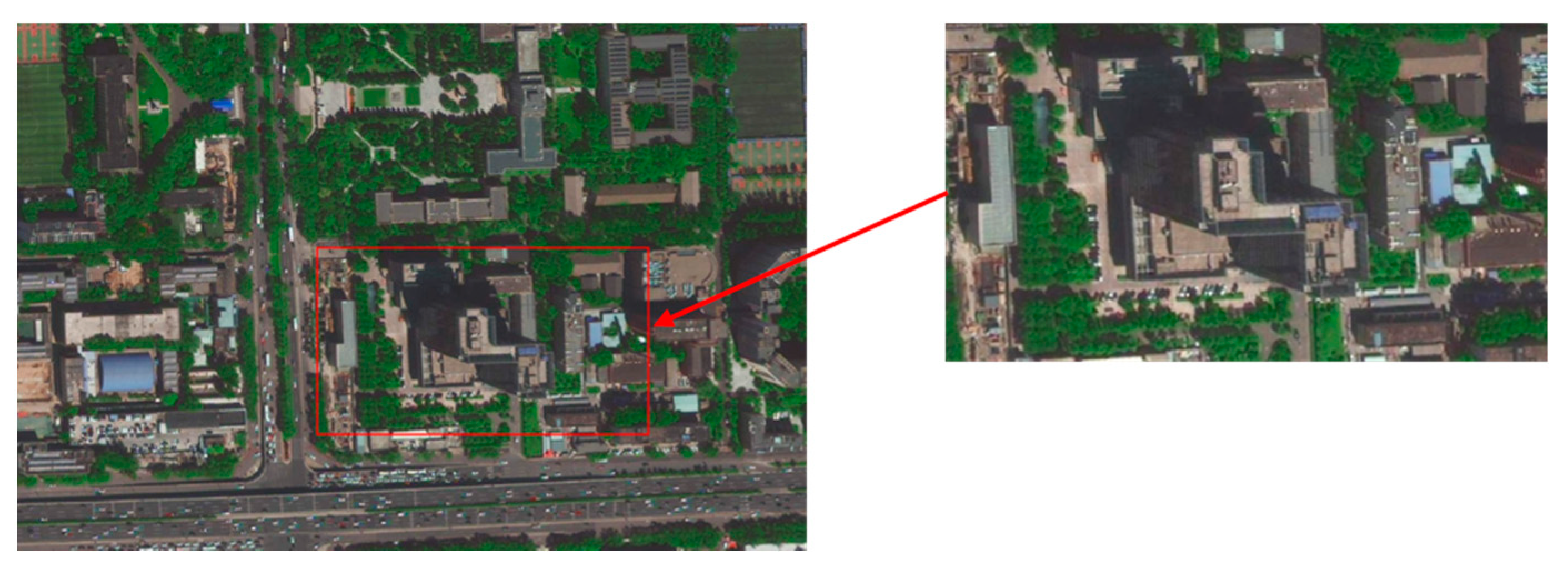
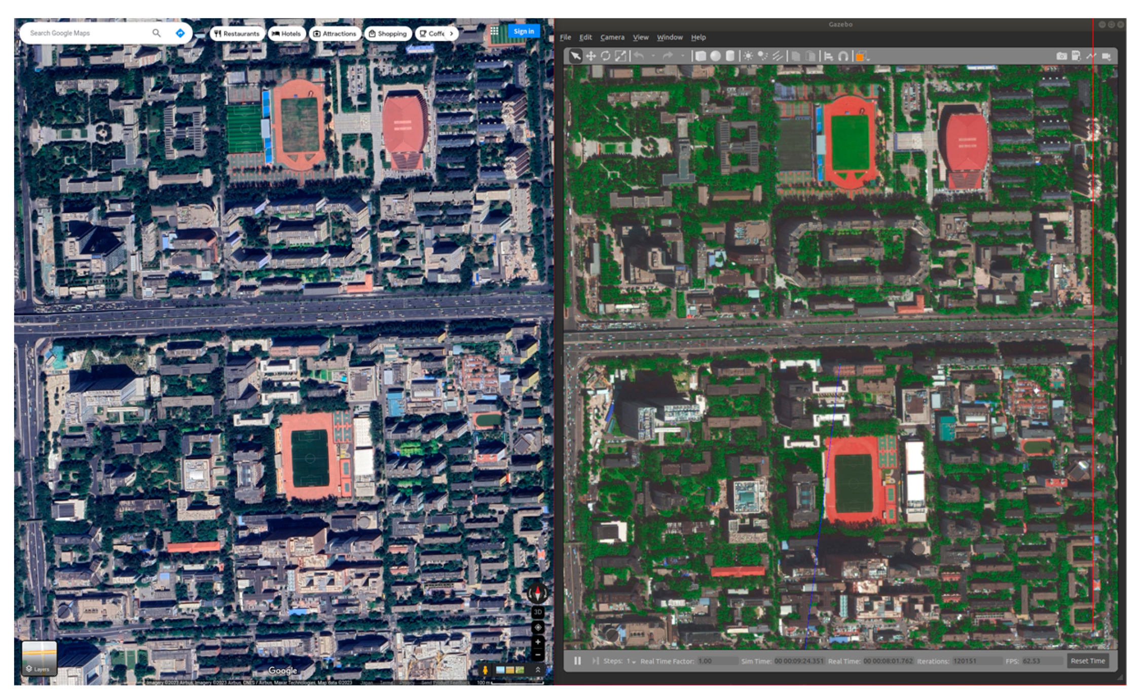
3.3. Google Earth for Gazebo

In the simulator, we use a Google commercial satellite map as a base map. To create a satellite map model and integrate it into a simulation world using Gazebo, which is a free robot simulation software program that provides high-fidelity physical simulations, and to achieve a complete set of sensor models and a user-friendly interaction between users and programs, we utilize the “Static Map” world plugin provided by Gazebo (https://gazebosim.org/ accessed in 1 October 2023). This plugin allows us to download satellite images in real time using Google’s “Static Maps API” and incorporate them into the simulation world. Please note that this plugin requires an internet connection as the satellite imagery is fetched during runtime. Since the “Static Map” world plugin generates the map model and inserts it into the simulation world at runtime, there is no need for a ground plane model. The satellite map model created using the plugin will serve as the terrain in the simulation environment. We insert some models from the Gazebo model database into the simulation world, as shown in Figure 7.

The parameters of the plugin are listed in

Table 2. Parameters of Google map.

Parameter	Description
center	The map center: latitude and longitude
World_size	The desired size of the world target to be covered
Model_name	The name of the map model
pose	The pose of the map model in the simulation
zoom	The zoom level
Map_type	The map type to be used, which can be a roadmap, satellite, terrain or hybrid. By default, it is set to satellite
Tile_size	The size of map tiles in pixels. The maximum limit for standard Google Static Maps is 640 pixels

.

3.4. Hardware Configuration of Simulation Platform

A Dell laptop with an Intel i7 9750H-2.6Ghz CPU is used as a simulation device. The field of view of the camera is 120° and the image size is 1920 × 1080 pixels. The gyroscope measurement range is 450°/s, and the zero bias stability of the gyroscope is set to 7°/h. The measurement range of the accelerometer is 20 g and the zero bias stability of the accelerometer is 14 μg. The measurement range of the UWB is 200 m, and the measurement error is 10 cm. We use the OpenCV 4.7 library for image processing, and Python3.7 is used for programming.

4. Simulation Result

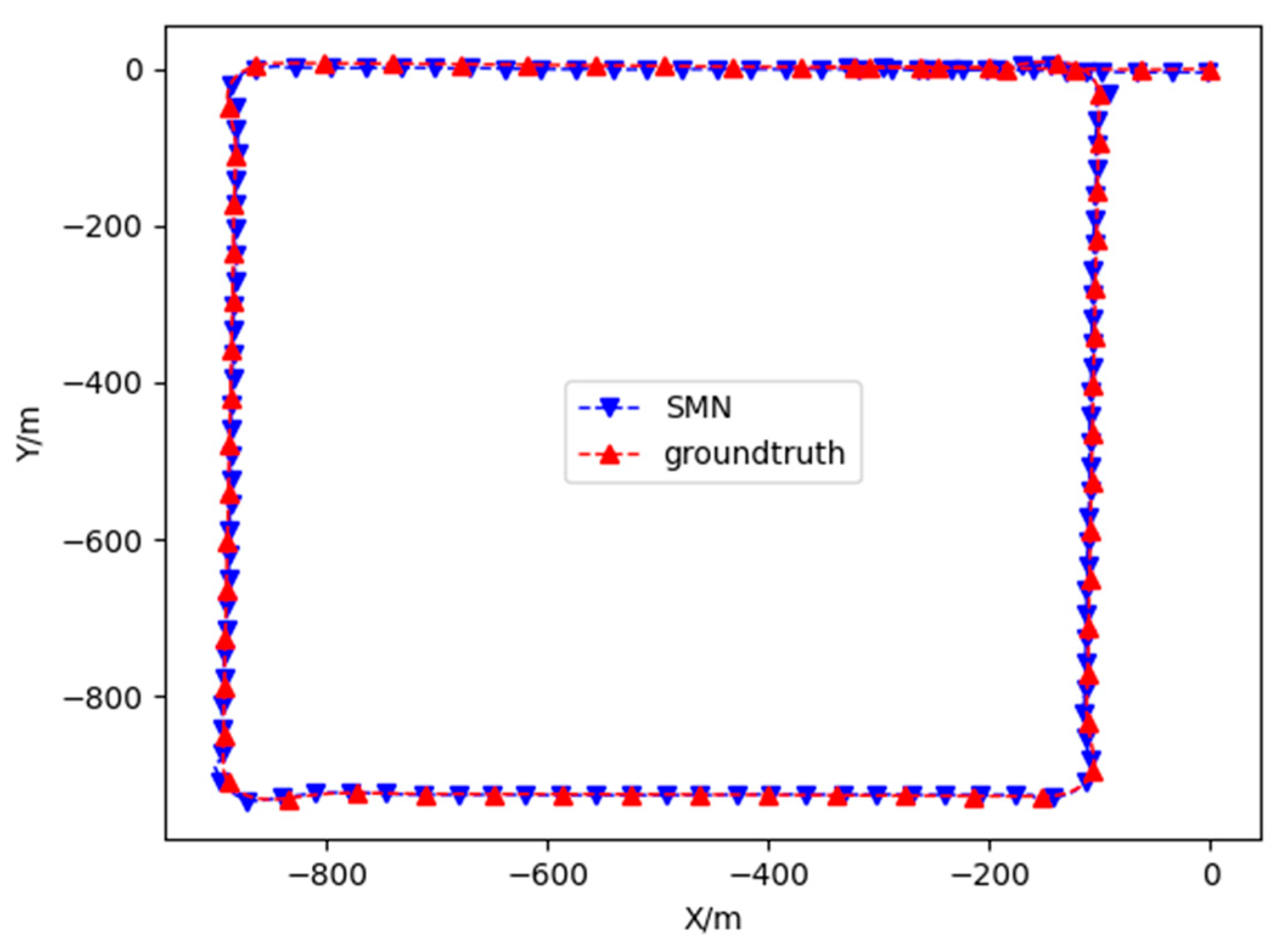
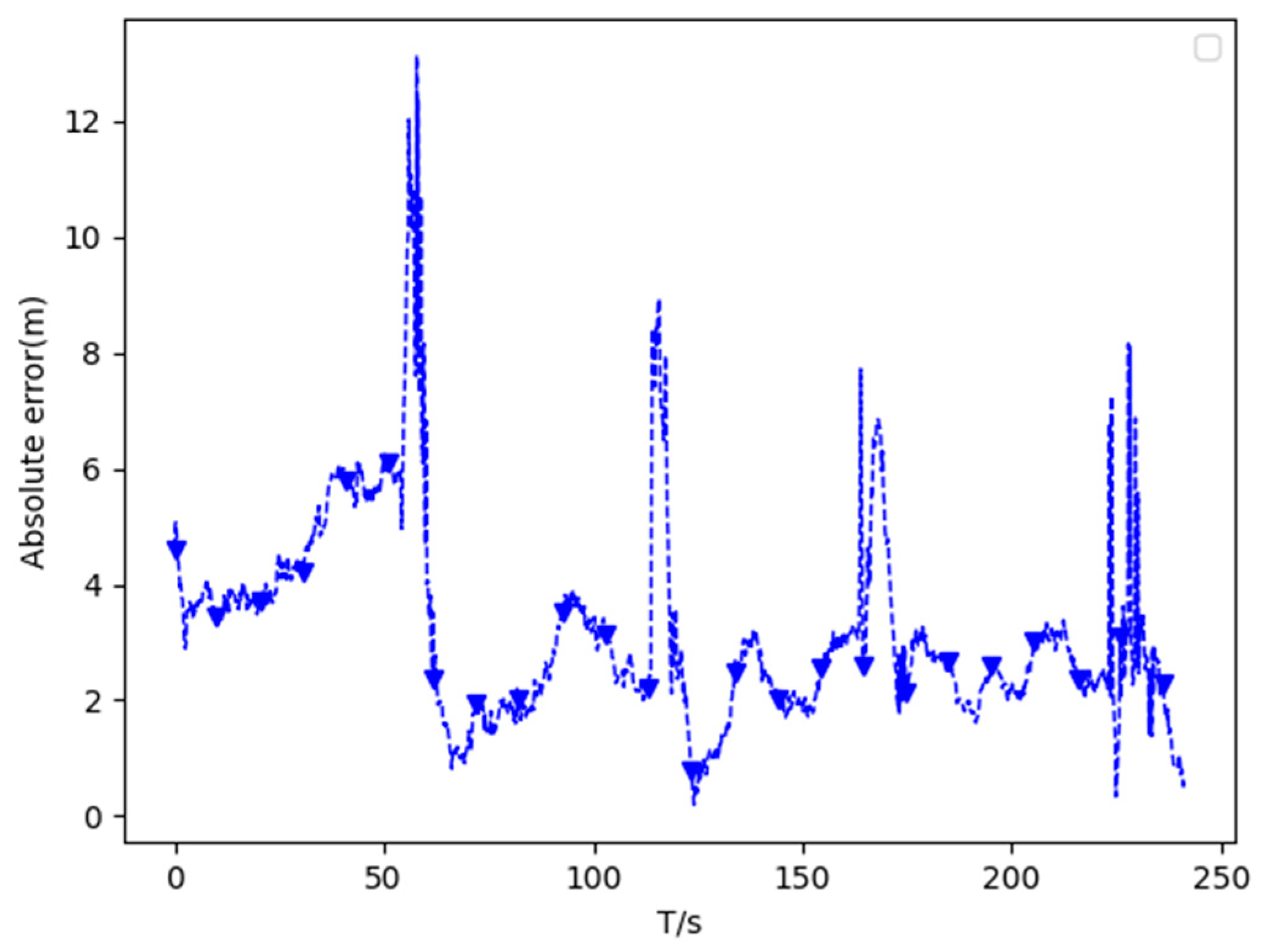
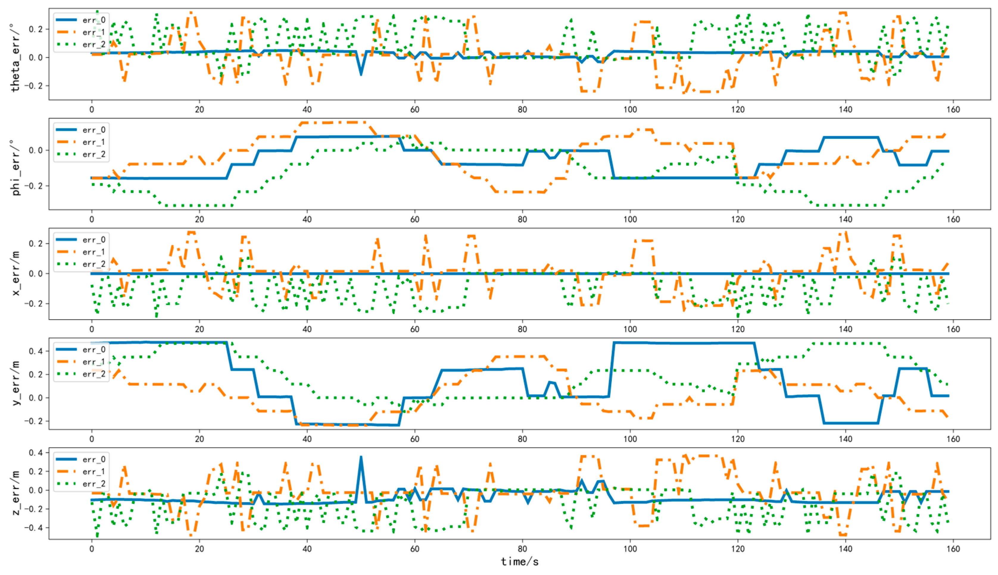
4.1. Simulation for ISMN

The ISMN is tested at Beijing University of Science and Technology, based on the 4546 × 3912 resolution Google civil and commercial satellite map. We aim to demonstrate the effectiveness of the simulation environment and localization algorithm by comparing the output of the ISMN with the truth values provided by the simulation environment. The ISMN outputs the longitude and latitude of the UAV. The simulation environment can provide true values of longitude and latitude for comparison. The mapping relationship between the real-time continuous images captured by the UAV and the satellite reference images is shown in Figure 8.

The result, shown in Figure 9 and Figure 10, indicates that when the UAV’s altitude is 800 m, the optimized reference map area and the input image overlap >90%, and the average positioning error is 3.1 m (<0.387% of the height) when the UAV flies smoothly. Moreover, when the UAV turns at a large angle (the attitude is ${30}^{\circ }$), the position error is 13.1 m. The experimental results indicate that the use of ISMN can achieve navigation in GNSS-denied environments.

4.2. Simulation for Relative Navigation

In the simulation, the swarm is composed of a leader and nine followers, the formation structure is as shown in Figure 11 and the distance between drones is set to 100 m. Taking the fourth drone as an example, the front camera can observe 0, 1 and 2, the left camera can observe 1, 3, 6 and 7 and the right camera can observe 2, 5, 8 and 9. The relative navigation based on the vision and UWB results is shown in Figure 12. We detect the IDs of adjacent drones through a camera and measure the relative line of sight and azimuth angle, obtaining the relative distance between UAVs through airborne UWB sensors. Based on the measurement results of the camera and UWB, we calculate the relative positions between UAVs using the theoretical tools discussed in Section 2.2. Using the truth values provided by the simulation system as a reference, according to Figure 12, the maximum relative position error is 0.75 m (<0.75% of the distance between adjacent drones). According to (19), the accuracy of the relative position mainly depends on the line of sight and azimuth angle measured by the camera. The error from UWB is only 10 cm, which is a small amount compared to the distance between machines. On the other hand, under the condition of a fixed angle error, the farther the distance between drones, the greater the relative navigation error.

5. Conclusions

This paper introduces a real-time simulator for navigation in GNSS-denied environments. The sensor models are established and imported to the simulator as a plugin. Based on Gazebo, a series of scenarios is simulated to facilitate the validation of the navigation algorithms in various environments. Addressing navigation challenges in denial environments, an inertial-aided scene matching navigation method is proposed for a camera working in a highly oblique scenario to improve the navigation performance. The position error is 13.1 m when the flight altitude is 800 m. Focusing on relative navigation, a method based on vision and UWB is proposed and the relative positioning accuracy is 0.75 m. Although we verify our simulation system in various environments, we find that there are many more outliers in complex conditions. In future research, we will tackle this challenge from the perspective of multirobot cooperative optimization in the continuous time domain. Moreover, relative navigation is closely related to the formation structure. The design of formation based on the relative navigation accuracy is worthy of in-depth research. In addition, we will develop hardware for robotic applications.

References

1. Zhou, X.; Wen, X.; Wang, Z.; Gao, Y.; Li, H.; Wang, Q.; Yang, T.; Lu, H.; Cao, Y.; Xu, C.; et al. Swarm of micro flying robots in the wild. Sci. Robot. 2022, 7, eabm5954. [Google Scholar] [CrossRef]
2. Soria, E.; Schiano, F.; Floreano, D. Predictive control of aerial swarms in cluttered environments. Nat. Mach. Intell. 2021, 3, 545–554. [Google Scholar] [CrossRef]
3. McGuire, K.N.; De Wagter, C.; Tuyls, K.; Kappen, H.J.; de Croon, G.C. Minimal navigation solution for a swarm of tiny flying robots to explore an unknown environment. Sci. Robot. 2019, 4, eaaw9710. [Google Scholar] [CrossRef] [PubMed]
4. Shan, M.; Wang, F.; Lin, F.; Gao, Z.; Tang, Y.Z.; Chen, B.M. Google Map aided Visual Navigation for UAVs in GPS-denied environment. In Proceedings of the 2015 IEEE International Conference on Robotics and Biomimetics (ROBIO), Zhuhai, China, 6–9 December 2015. [Google Scholar] [CrossRef]
5. Prometheus. Available online: https://github.com/amov-lab/Prometheus (accessed on 1 October 2023).
6. XTDrone. Available online: https://github.com/robin-shaun/XTDrone (accessed on 1 October 2023).
7. Xiao, K.; Ma, L.; Tan, S.; Cong, Y.; Wang, X. Implementation of UAV Coordination Based on a Hierarchical Multi-UAV Simulation Platform. Advances in Guidance, Navigation and Control; Lecture Notes in Electrical Engineering; Springer: Singapore, 2022; Volume 644. [Google Scholar] [CrossRef]
8. Dai, X.; Ke, C.; Quan, Q.; Cai, K.Y. RFlySim: Automatic test platform for UAV autopilot systems with FPGA-based hardware-in-the-loop simulations. Aerosp. Sci. Technol. 2021, 114, 106727. [Google Scholar] [CrossRef]
9. Wang, S.; Dai, X.; Ke, C.; Quan, Q. RflySim: A rapid multicopter development platform for education and research based on pixhawk and MATLAB. In Proceedings of the 2021 International Conference on Unmanned Aircraft Systems (ICUAS), Athens, Greece, 15–18 June 2021; IEEE: Piscataway, NJ, USA, 2021; pp. 1587–1594. [Google Scholar]
10. Qin, T.; Li, P.; Shen, S. VINS-Mono: A Robust and Versatile Monocular Visual-Inertial State Estimator. IEEE Trans. Robot. 2017, 34, 1004–1020. [Google Scholar] [CrossRef]
11. Balamurugan, G.; Valarmathi, J.; Naidu, V.P.S. Survey on UAV navigation in GPS denied environments. In Proceedings of the International Conference on Signal Processing, Communication, Power and Embedded System (SCOPES), Paralakhemundi, India, 3–5 October 2016; pp. 198–204. [Google Scholar]
12. Mei, C.; Fan, Z.; Zhu, Q.; Yang, P.; Hou, Z.; Jin, H. A Novel Scene Matching Navigation System for UAVs Based on Vision/Inertial Fusion. IEEE Sens. J. 2023, 23, 6192–6203. [Google Scholar] [CrossRef]
13. Xia, L.; Yu, J.; Chu, Y.; Zhu, B.H. Attitude and position calculations for SINS/GPS aided by space resection of aeronautic single-image under small inclination angles. J. Chin. Inert. Technol. 2015, 350–355. [Google Scholar] [CrossRef]
14. Saska, M.; Baca, T.; Thomas, J.; Chudoba, J.; Preucil, L.; Krajnik, T.; Faigl, J.; Loianno, G.; Kumar, V. System for deployment of groups of unmanned micro aerial vehicles in GPS-denied environments using onboard visual relative localization. Auton. Robot. 2017, 41, 919–944. [Google Scholar] [CrossRef]
15. Walter, V.; Staub, N.; Franchi, A.; Saska, M. UVDAR System for Visual Relative Localization With Application to Leader–Follower Formations of Multirotor UAVs. IEEE Robot. Autom. Lett. 2019, 4, 2637–2644. [Google Scholar] [CrossRef]
16. Güler, S.; Abdelkader, M.; Shamma, J.S. Peer-to-Peer Relative Localization of Aerial Robots With Ultrawideband Sensors. IEEE Trans. Control. Syst. Technol. 2020, 99, 1–16. [Google Scholar] [CrossRef]
17. Xiang, H.; Tian, L. Method for automatic georeferencing aerial remote sensing (RS) images from an unmanned aerial vehicle (UAV) platform. Biosyst. Eng. 2011, 108, 104–113. [Google Scholar] [CrossRef]
18. Redmon, J.; Farhadi, A. Yolov3: An incremental improvement. arXiv 2018, arXiv:1804.02767. [Google Scholar]
19. Couturier, A.; Akhloufi, M.A. A review on absolute visual localization for UAV. Robot. Auton. Syst. 2021, 135, 103666. [Google Scholar] [CrossRef]
20. Cesetti, A.; Frontoni, E.; Mancini, A.; Ascani, A.; Zingaretti, P.; Longhi, S.A. visual global positioning system for unmanned aerial vehicles used in photogrammetric applications. Intell. Robot. Syst. 2011, 61, 157–168. [Google Scholar] [CrossRef]
21. Conte, G.; Doherty, P. Vision-based unmanned aerial vehicle navigation using geo-referenced information. EURASIP J. Adv. Signal Process. 2009, 10, 387308. [Google Scholar] [CrossRef]
Figure 1. Architecture of the simulator.
Applsci 13 11278 g001
Figure 2. ISMN system architecture.
Applsci 13 11278 g002
Figure 3. Reference map from INS propagation.
Applsci 13 11278 g003
Figure 4. Inertial-Aided Georeference.
Applsci 13 11278 g004
Figure 5. Camera imaging plane.
Applsci 13 11278 g005
Figure 6. Measurement scheme for multiple UWB nodes in an infinite loop.
Applsci 13 11278 g006
Figure 7. Google map in simulation world.
Applsci 13 11278 g007
Figure 8. Real-time mapping between images captured by the UAV and the base map.
Applsci 13 11278 g008
Figure 9. The trajectory of ISMN simulation.
Applsci 13 11278 g009
Figure 10. The absolute error of ISMN simulation.
Applsci 13 11278 g010
Figure 11. Formation structure.
Applsci 13 11278 g011
Figure 12. Relative navigation result.
Applsci 13 11278 g012