Abstract
A robot can accurately localize itself and navigate in an indoor environment based on information about the operating environment, often called a world or a map. While typical maps describe structural layouts of buildings, the accuracy of localization is significantly affected by non-structural building elements and common items, such as doors, appliances, and furniture. This study enhances the robustness and accuracy of indoor robot localization by dynamically updating the semantic building map with non-structural elements detected by sensors. We propose modified Adaptive Monte Carlo Localization (AMCL), integrating object recognition and map updating into the traditional probabilistic localization. With the proposed approach, a robot can automatically correct errors caused by non-structural elements by updating a semantic building map reflecting the current state of the environment. Evaluations in kidnapped robot and traditional localization scenarios indicate that more accurate and robust pose estimation can be achieved with the map updating capability.
1. Introduction
Real-time localization is one of the key techniques used in robotization, which estimates the location and orientation of a mobile robot within its operating environment by aligning data from a combination of sensors and information of the environment stored in a map. The accurate and robust calculation of the location, as well as orientation, in the map provides an essential basis for a robot to determine appropriate actions in given situations [1]. With the increasing utilization of indoor mobile robots, recent studies have presented various techniques to determine the robot poses within built environments [2,3,4]. In its most basic approach, a wheel-based mobile robot can estimate its position based on wheel encoders. Despite its simple implementation, pose estimation using a wheel encoder can suffer from drift. As another class of approaches, studies have presented methods that rely on landmarks (such as BLE sensors [5], RFID sensors [6], and visual markers [7]) installed in the environment. Even though these landmarks can explicitly indicate known locations, these approaches can also suffer significantly from even slight changes made to the configuration of the environment. Deviations from the initial setting, such as additional interior partitions and the relocation of large furniture and electronic appliances, dramatically reduce the accuracy, which then requires recalibration of the entire setting for localization. Many probabilistic methods were then proposed recently to allow for the estimation of possible robot poses by fusing data from multiple sensors [8]. Because of robustness in response to changes in the environment, probabilistic approaches have the potential to overcome the limitations of deterministic localization methods. Monte Carlo Localization (MCL) [9] continuously generates the distribution of arbitrary robot poses and selects samples from the particles of highly probable robot poses. This approach uses pose data, previously built occupancy grid maps, sensor data, and Kullback–Leibler divergence (KLD)-based sampling. Adaptive Monte Carlo Localization (AMCL) [10] is one of the most widely used variations derived from MCL. A Robot Operating System (ROS)-based implementation of AMCL [11] has been applied in many studies [12,13] that successfully fused data from multiple sensors (e.g., 2D laser scan, IMU, wheel encoder) to accurately estimate robot poses.
Despite these advances, most of the approaches in robot localization were developed with the assumption that the operating environment is static. A typical map reflecting the knowledge about the present environment is a two-dimensional grid map depicting unchanging structural elements, such as walls, floors, and ceilings. In a typical building environment, however, non-structural building elements and common items (e.g., temporarily loaded materials, doors, appliances, and furniture) also exist, which change location occasionally and consequently significantly impact the accuracy of localization [14]. In order to overcome the impact of these non-structural elements that are not being represented within a map, this study proposes a method that allows a mobile robot to continuously update the map with objects it encounters during navigation and correct possible positioning errors automatically. More specifically, we propose a modification to the traditional AMCL localization method to integrate image-based object recognition, point cloud processing, and map updating. Then, we evaluated the performance of the modified AMCL method based on a conventional localization scenario, where a robot starts the navigation from a known location, and also a kidnapped robot scenario, where a robot has to find its location without knowledge about prior locations.
2. Literature Review
2.1. Indoor Robot Localization Techniques
Robot localization is the process of estimating the position and orientation of a mobile robot with respect to the environment, which is an important task for mobile robots as it is essential for path planning [15]. Many technologies are used to localize mobile robots, and they are usually divided into relative positioning and absolute positioning. The relative (local) localization uses internal sensors (such as wheel encoders, inertial sensors, and digital compasses) to estimate the robot’s pose [16]. The absolute (global) localization uses external sensors (such as cameras and lasers) that enable direction calculation of the location with respect to the environment. The relative localization of the robot is estimated based on the information obtained through the integration of different sensors. The integration is initiated at the starting position and continuously updated throughout time. Relative position measurement techniques are widely used because of their low cost and faster pose estimation. However, relative positioning cannot be used to measure long distances due to errors, such as wheel slippage and other unbounded errors, which continue to accumulate with increases in the distance traveled by the robot [15]. Wheel odometer-based localization is a navigation method for relative positioning techniques in the mobile robot field, known as dead reckoning, which uses a rotary encoder that measures the rotation of the wheels to calculate the pose of the robot. It is very simple, inexpensive, and has good accuracy over a short range and short term, but it incurs a high level of uncertainty in cumulative position estimation over time due to wheel-slip, changes in wheel dimensions, and misalignment. The level of uncertainty could be mitigated by combining multiple sensors optimally and generating better position estimation through Kalman filter fusion techniques [17,18]. The Inertial navigation systems (INSs) can also be utilized to estimate the pose of a robot with respect to the starting point. They typically include IMUs, which are equipped with accelerometers, gyroscopes, and magnetometers to calculate the position, direction, and velocity of a moving object. The advantages of the inertia sensors include simple implementation, lower prices, and utilization without prior knowledge about the environment [19]. Even though INS-based approaches do not require external references for positioning, they are vulnerable to cumulative errors that can lead to large localization errors in a short period of time. This is because the mathematical integral of the acceleration with respect to time should be calculated to estimate the pose. The small errors in acceleration and velocity accumulate over the integral calculation and produce increasingly inaccurate position estimates. The magnetometer sensor in the IMU could provide the robot’s absolute heading by measuring the earth’s magnetic field; however, the earth’s magnetic field is often distorted near metal objects, which makes it inappropriate for indoor applications [20]. Therefore, any type of inertial sensor is not appropriate for long-term position estimation.
Unlike relative localization, absolute localization does not suffer from error accumulation because the calculation of the current pose does not depend on the previous poses. However, the measurement of small movements using external sensors may not be as accurate as that with internal sensors [19]. One of the most popular external sensors for absolute localization is GPS (Global Positioning System). Its performance is negatively affected by the canopy, bad weather, and building structures blocking the signal strength to the GPS receiver [21]. This aspect makes GPS unreliable for the indoor localization of objects, which is the focus of this paper. Video cameras are also utilized for the absolute localization of mobile robots. Camera-based methods can achieve relatively accurate positioning with a low cost, low weight, and low power consumption. Visual sensor data from cameras provide rich information essential for localization, mapping, obstacle detection, and path planning without the need for merging other sensors. However, cameras suffer from the influence of lighting conditions, especially in an outdoor environment, and distortion due to fast movement, in addition to its view being narrow [21]. As another approach for absolute localization, a laser range finder measures relative distances between a robot and objects in its surroundings with the time of flight of the pulse. The distances can be used to generate a metric map or to determine the location of the robot within the map of the known environment. Landmark-based absolute localization attaches landmarks as fixed features that mobile robots can directly match with known locations. It is classified into an artificial landmark or natural landmark. Artificial landmarks are objects or shapes that are placed in the environment for the sole purpose of robot localization, while natural landmarks are features that already exist in the environment, which can be used for localization. The artificial landmarks can be geometric shapes or objects and other additional information in the form of bar-codes [22]. Many approaches explicitly mark the indoor environment by laying down magnetic lines that a robot can follow [23] or placing QR-coded markers that visually represent known locations [7]. Although these approaches can be highly reliable in a static environment, those markers cannot cope with changes made to the initial setting. The relocation of common items, such as furniture and large electronic appliances, can block the line-of-sight of the mark or block signals prohibiting positioning.
Many localization techniques were then proposed to enhance the accuracy and robustness based on multiple sensor fusion and a probabilistic approach. Multi-sensor fusion combines multiple sensor data, such as an RGB camera, RGBD camera, LiDAR, radar, and other sensors that measure relative and absolute localization [24]. The most well-developed probabilistic approaches are based on a Bayes Filter. From EKF (Extended Kalman Filter) to a particle filter, it recursively updates the conditional probability distribution over the state space of the robot to estimate its pose. In particular, representing the posterior distribution based on a set of samples or particles, the particle filter-based approaches [25], also known as MCL methods, are most widely used for robot localization since they could deal with nonlinear and non-Gaussian problems, and almost arbitrary distributions can be represented. However, it requires a sufficiently large number of particles to cover the state space to generate pose estimates with acceptable accuracy and success rates. Hence, MCL methods may perform poorly if the size of the sample set is small in a large environment and the complexity, and memory cost of this kind of method will grow significantly as the state space expands [26]. Furthermore, this approach relies on the consistency between the given map and real environment. Therefore, it becomes important that the robot be able to deal with the changes in the environment over time [27]. Especially, the construction environment keeps changing over time, and various objects in the construction environment should be dynamically updated in the map. For autonomous robot systems to effectively operate based on a building environment, they must be able to refer to or derive a semantic model of the environment [28]. Some researchers have made it possible for the robot to access project information contained in a Building Information Model (BIM), which is a comprehensive database of a built environment [29].
2.2. Creating Indoor Maps for Robot Localization
This section reviews studies that have created environment maps that can be used for robot operations, not limited to localization. Numerous studies have proposed different techniques and approaches using the appearance, geometric, and topological features contained in the environment for creating a two-dimensional (2D) map and localizing robots in spaces. A statistical approach was proposed in [30] for creating 2D metric maps based on landmark features for large-scale indoor environments using the motion and perception of a mobile robot. The approach can estimate both the robot’s position and mark the location of the landmarks in an indoor environment to create a map. However, the approach requires a human to identify these landmarks and control the robot. The authors of [31] created 2D maps that contain both topological and geometric features by performing SLAM and localizing the robot using the topological features or objects in an unknown space. This approach may experience difficulties in an open space with little topographical features (e.g., a plain wall with no edges) that the robot can recognize easily. Ref. [32] presented a multilayered map by first creating a 2D metric map with geometric information and transforming the data into a topological map. The transformation process described in the study adjusts the potential obstacle grid of the metric map to create topological features of the environment. The authors of [33] presented a view-based mapping system to incrementally build maps with geometric features for both outdoor and indoor environments as the robot performs SLAM in the environment. In this approach, a map was generated by continuously stitching camera views using geometric features. Ref. [34] proposed a loop-closure detection approach using a memory management mechanism to reduce the time to create maps for large areas. Similar to that in reference [33], the loop closure detection allows a robot to link previously seen views to the current view in real time during SLAM to create a geometric map. In [35], a graph-based SLAM solution was proposed to create geometric maps for indoor environments based on the memory management approach in [34] to cater to the multi-session mapping of large areas where gross errors in odometry and the “kidnapped robot” situation might occur.
Even though several studies have created 2D geometric maps for robot task planning and navigation, recent studies have attempted to incorporate important non-geometric information about the environment in maps to facilitate the intelligent behaviors of robots. Many studies proposed methods of combining semantic information with geometric and topological features of spaces to further improve a robot’s understanding of a space for performing tasks. Ref. [36] proposed a multi-hierarchical approach using sensor data from a mobile robot to build semantic maps that includes both spatial and semantic information of spaces for performing tasks, such as room classification according to observed objects. This multi-hierarchical approach consists of a metric map connected to global topological features and is linked to the semantic representations of the space through an anchoring process that allows the robot to draw inferences from symbolic data to perform complex tasks that requires semantic information. Ref. [37] extended the approach in [36] to present ways in which a robot can generate new goals based on predefined semantic knowledge in the metric map to deduce new information for performing complex task planning and ignore less important information. Similar to that in [36], a Bayesian hierarchical probabilistic approach was presented in [38] to classify and infer semantic information about a space by linking commonly found objects and spatial features in that space to create a semantic map with spatial features. Ref. [39] acquired 3D scan data of the spatial features of spaces by performing 6D SLAM with a mobile robot to create a 2D semantic map. The approach semantically labels and localizes objects, as well as spatial features in a scene, based on a previously trained classifier to create a map that includes both spatial and semantic information. Ref. [40] proposed a method to create a semantic map that includes spatial information from a metric map by semantically modeling the objects commonly found in the place. The objects are identified and trained using image processing techniques and a trained supervised learning algorithm. Ref. [41] presented an approach that performs SLAM and combines both metric and topological features with the semantic information of spaces to create a semantic map. The approach uses the ontology of the space and the interactions between a human and a robot to create the semantic information that the robot can use for planning and executing tasks.
3. Objective and Scope
Even though typical maps provided to robots describe structural layouts of buildings, the accuracy of localization is significantly impacted by non-structural building elements and common items, such as doors, appliances, and furniture, which a robot can recognize using its sensors. However, none of the mentioned approaches have enhanced robot localization by dynamically updating the semantic building representation with non-structural elements. It is clear from related works on semantic maps and object recognition that there have been interesting solutions and approaches proposed to improve robot localization. State-of-the-art studies have not proposed an approach that considers altering the navigation map dynamically. This study presents a new method to enhance the accuracy of indoor robot localization by automatically updating the environment state in a semantic 3D building map. This study also presents a modified AMCL that integrates object recognition and map updating based on traditional probabilistic localization. For that, we developed a robot localization system that analyzes real-time data from sensors, detects and classifies objects using object-recognition techniques, acquires geometric information about detected objects using the depth point cloud, and creates a semantic building map reflecting the current environment state.
4. Methodology
4.1. Overview of the Modified AMCL with Map Updating
This section describes the overview of the proposed modified AMCL with real-time map updating. As shown in Figure 1, the proposed process is composed of three major components, including semantic building map creation, map updating with sensor-based object detection, and AMCL localization with the updated map. When localization or navigation begins, (1) semantic building model creation generates a 3D semantic building model and a 2D AMCL map that can be used by an autonomous robot. A BIM model, as a building lifecycle database, contains comprehensive geometric and non-geometric information about a building. A semantic building model in our study is a ROS-compliant building model that can describe both static elements (e.g., walls, floors, ceilings) and dynamic elements (e.g., doors, furniture, large electronic devices) in a way that can be interpreted by a robot. We utilized the IFC-to-URDF convertor used in our previous work [42,43] that parses information in a BIM model and augments additional information to generate a semantic 3D building model. Based on the semantic 3D building model, a 2D AMCL map is generated as the essential input for AMCL-based localization and navigation. The semantic 3D building model is updated when a robot detects the presence of non-structural elements, such as doors or furniture, and estimates their poses within the building, and the 2D AMCL map is updated accordingly to reflect the observed changes. Depending on the characteristics of the objects, the 2D AMCL map can be directly updated without updating the 3D model. For example, the state of a swing door can be accurately described by updating the door angle around the known door hinge coordinate stored in the semantic 3D model. A 2D map showing the area occupied by the door can be generated based on the 3D model. In this way, an accurate 2D map can be created even with only partial observation of the elements. However, it is difficult to accurately estimate the poses and boundaries of non-building elements (such as a sofa, table, bed) without fully observing the entire element from all angles, which would require excessive additional movements. For non-building elements, our study estimates the partial boundary of the elements that can impact the accuracy of localization and updates the 2D AMCL map directly without changing the 3D model. However, accurately updating the 3D building model with non-building elements would also be possible if the information about the items could be provided in advance. (2) Sensor-based object recognition utilizes sensors attached to the mobile robot to detect the presences of objects that can impact localization and estimate their boundaries to be updated in the 2D/3D maps. From the RGB images, the robot detects and classifies objects using object-recognition techniques. Then, it acquires geometric information on the detected objects using depth point cloud data. The presence and states of the detected elements are then updated in the 2D/3D maps reflecting the current state of the environment. (3) AMCL localization with an updated map is a conventional localization method utilizing the given map of the environment. AMCL is a probability-based 2D robot localization algorithm, also known as particle filter localization, which uses many particles to track the pose of a robot in a known map with an adaptive (or KLD sampling) Monte Carlo localization approach. Each particle in the particle filter represents a distribution of possible states, considered a hypothesis of where the robot is. The regions with many particles indicate an increased probability of the robot’s actual position, whereas regions with fewer particles are unlikely to be where the robot is. The algorithm usually initializes uniformly distributed random particles over the known map because the robot has no knowledge of its pose on start-up and assumes that it is equally likely to be anywhere on the known map. The algorithm also assumes the Markov property that the current state’s probability distribution depends only on the direct previous state (not any states before that). This only works if the environment is static and does not change through time. Typically, on start-up, the robot has no information on its current pose, and thus, the particles are uniformly distributed over the configuration space. Subsequently the particles move to predict the new state at each moment of robot movement. The particles are also resampled based on recursive Bayesian estimation whenever the robot sensor detects something, and it represents how well the detected data correlate with the predicted state. In other words, resampling means discarding particles that do not match the sensor observation and producing more particles that are more consistent with the sensor measurement. This is because the robot does not always behave in a predictable way; thus, there needs to be corrections to the pose based on sensor data. In the end, hopefully, most particles should converge to the actual robot pose. Therefore, the AMCL algorithm estimates the position and orientation of a robot as it moves and senses the environment in the given map.
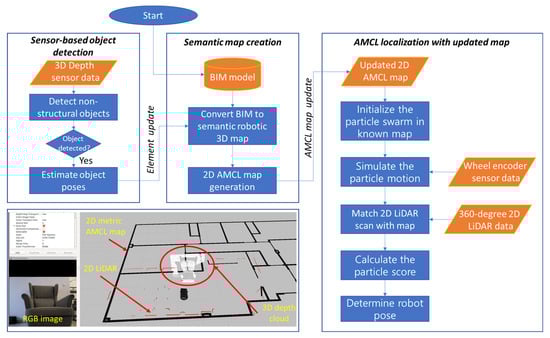
Figure 1.
Overall framework.
4.2. Examples of Localization Errors Caused by Non-Structural Elements
Due to the reliance on geometric features of the environment, probabilistic-based location algorithms could easily report erroneous localization poses when the surface shapes of different objects are similar. For example, a sofa not presented in a map could be interpreted mistakenly as a wall due to its large and flat front surface, as shown in Figure 2a. Because of this error, the entire map will be incorrectly offset toward the wall. The green particle swarm around the robot represents the best guess of the AMCL algorithm regarding where the robot is, which is incorrect. There are fewer correct particles than incorrect particles, and thus, the algorithm chose an incorrect pose as its localization. Figure 2b shows another example of inaccurate AMCL localization due to closed doors being recognized as walls. The navigation routine could plan routes through the doors if the frames are left open as spaces. However, when doors are closed, their previously empty space in the map is filled, allowing the closed doors to easily be mistakenly interpreted as part of a contiguous wall. As a result, a robot may determine its pose to be in another location in the building where there are three doors and continuous walls along the hallway. This type of layout is very difficult for a robot when subjected to the “kidnapped robot” problem [30], which arises when a robot is placed within the building and not given a starting pose or is relocated to another place in the building. Our study attempts to address these limitations by recognizing the types of objects, estimating their poses, and augmenting the information in the AMCL map during real-time localization.
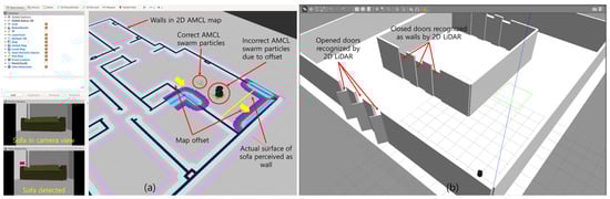
Figure 2.
AMCL localization errors (a) due to the interpretation of the sofa front as a wall and (b) doors being mistakenly recognized as a contiguous wall.
4.3. Semantic Map Creation from BIM
A robot’s operating software should internally maintain a map, which is an internal representation of its operating environment. From the map, the robot can retrieve geometric and semantic information required for task planning and execution. In cases of AMCL localization, the map should provide the geometric information of the environment (as shown in the 2D AMCL map in Figure 2a) and key coordinates, such as the initial location and target destination. In addition to the structural elements, our study incorporates dynamic non-structural elements, such as doors and furniture, in order to represent the environment with details sufficient for robot operations. For example, the static door element modeled in BIM (Figure 3a) describes a door with a static solid model with annotations showing possible door swings. However, as shown in Figure 3b, the main body of the door needs to be described as a dynamically movable element that can interact with a robot. In order to overcome the limitation, our study describes a building in a URDF format to describe static and dynamic elements within the robot operating environment. The URDF is a format that is commonly used for precise description of the dynamic actions of robot parts. A URDF file expresses a robot with its subparts as links and joints that describe the relationship between links. We utilized the IFC-URDF convertor from our previous work [43] to generate a URDF building model from a BIM model. Ref. [43] provides technical details about the BIM-URDF conversion used in this study. There are four major steps required for the generation of a dynamic URDF building model.
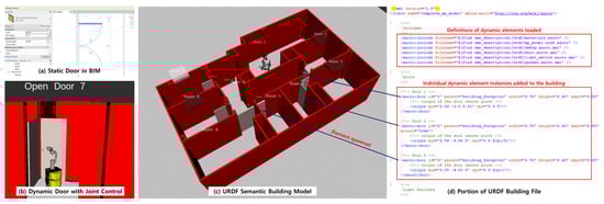
Figure 3.
URDF building model creation for semantic localization of (a) conventional static door element in BIM, (b) dynamic door element with joint control, (c) 3D URDF building model with static and dynamic building elements, and (d) part of the URDF building file presenting dynamic building elements.
Step 1. BIM-based building model creation: This first step is a traditional process to model a 3D BIM model that contains project information, including geometric information of individual building elements and properties of the building elements. This process can use commercially available BIM authoring tools.
Step 2. Conversion of building element information using IFC-URDF converter: This step converts the information about individual building elements to a ROS-compliant URDF format. This is done to describe both the static and dynamic aspects of building elements required for robot operations. Ref. [43] created the IFC-URDF converter that generates URDF files from an IFC file. The conversion first extracts shapes of static elements, such as walls and floors, from an IFC file and generates one URDF file. This URDF file describes static building elements as links connected with fixed joints. Using fixed joints, the one congregate object combining all static elements remains static during robot operations. However, elements with dynamic behaviors, such as doors and windows, are expressed in a different way. After extracting geometric information of the dynamic elements, the relationship between their hosting element links and the dynamic joints are specified to define their possible motions. As shown in Figure 3c, doors are connected to walls with revolute joints that allow door swings around the door hinges when a robot attempts to open the door. Moreover, any other project information required for robot task planning can be stored separately in other formats, such as XML, which a robot can parse. As a result, step 2 generates one URDF file for all static building elements, a URDF file for each dynamic element, and multiple XML files for other project information that are combined in step 3.
Step 3. Integration of converted URDF files into a robotic building world: This step combines the converted files from step 2 to generate a robotic building world that becomes a robot’s internal representation of the environment. Figure 3d shows how parametric door URDF files can be attached to the main URDF building model. The initial building world may contain all the project information, but a partial building world can be loaded on a robot’s operating software to reduce the computational burden of handling a large amount of project information. Partial building worlds can be customized for different robotic tasks and uploaded through wireless or wired connections.
Step 4. Retrieval of project information for robot task planning: In this last step, a robot performs tasks utilizing the information in the building world. Robot actions can be triggered by a user’s comments, such as “navigate to room 1”, “open doors and windows in room 3”, and “measure the current angle of door 3”. Then, the results of the robot actions can be reflected in the internal building representation by updating the building world model.
4.4. Object Detection
The object detection part of the proposed framework uses a neural net-based computer vision algorithm called You Only Look Once (YOLO) [44]. The YOLO algorithm is based on a deep convolutional neural network, which provides robust image recognition of a predefined list of objects and operates based on unstructured, arbitrary images, identifying objects for which it has been trained. The images are divided into grid cells to determine the class and represent a probability of the likelihood of identification (a confidence weight of the neural net) and a bounding box encompassing the recognized object. These processes are executed through the same neural network structure and were trained to recognize 80 common household objects, including people, bicycles, cars, dogs, and cats. All of the objects targeted for this study, such as chairs, sofas, tables, refrigerators, and people, were included in the pre-trained set of weighting values except for the doors. Due to the importance of doors in this study, custom training for the neural network was undertaken. A subset of door images was taken from the image list from [45], as well as more than 50 images taken by the authors from the test building of the actual doors being tested. This combined image set, comprising more than a hundred images of doors in different positions and lighting conditions, was then used as the neural network’s training set. Because of the extreme computational demands of neural network training, an NVIDIA Tesla K80 graphical processing unit (GPU) made available via Google Colab [46] was used to compute the training weights. All images used for training were annotated, which is the process of specifying the bounding coordinates within the image of the object to be recognized (for this study, the door) along with a corresponding label (in this case, simply “door”). Annotations for this dataset were carried out by hand for each image. All images used for training were then specified within an input training file, along with the classification labels and other training parameters and hyper-parameters. With these files uploaded to Google Colab, the training could proceed, taking roughly 12 h of computation time on the GPU. This resulted in a weights file, which was then used for the YOLO during execution of the software stack.
4.5. Location and Boundary Estimation Using RGBD Point Cloud
Localization and boundary estimation is performed after the presence of an object is detected by YOLO image-based object detection. Figure 4 presents a point cloud processing pipeline that extracts the location and boundary of the object detected by YOLO. This pipeline is used to determine the locations and boundaries when general objects, such as a sofa, are detected. The pipeline begins with obtaining a set of RGBD point cloud data from a depth camera (Step 1). This is either passed to the pipeline as an ROS PointCloud2 object, or it is passed as a file path to a point-cloud (.pcd) data file, which can be loaded into memory. The next two steps are performed separately and in parallel. A set of point clouds representing the floor is removed (Step 2). Using plane segmentation of the PCL library [47], planar surfaces are identified and organized in the order of their size, with the largest planes identified first. If one or more planes are found to be within an absolute tolerance of the vertical (z-axis) basis vector, they were considered floors. The tolerance factor was experimentally set after trial-and-error to be 0.97 for real-world experiments and 0.99 for simulations. This process has the effect of reshaping the point cloud, converting it from one point per pixel (640 × 480 in these experiments) to a single dimensional “flat” data structure. Because of this re-shaping, the cropping of the YOLO-identified bounding box (Step 3) must occur in parallel with (rather than after) the floor plane segmentation. With this process, the full point cloud is cropped to what YOLO has identified as the object. This provides a starting point for further segmentation. In addition, it cannot occur before plane segmentation since a large amount of the cloud is removed during bounding box cropping, often leaving too few floor points to qualify as a plane. Thus, these two processes are performed in parallel, and then, a union of the points is generated in Step 4 of the pipeline. Statistical outliers, which are points that statistically likely do not belong (i.e., noisy points), are removed in Step 5. A process of grouping together points that likely belong to the same object is performed in Step 6. This step is called Euclidean Clustering of PCL library [48], and it generally results in several point-clouds, each of which is indicative of an object. YOLO generally draws a tight bounding box around the object it identifies and the point-cloud that is cropped according to this bounding (Step 3). Thus, the largest object after Euclidean clustering is chosen as the object of interest. The point cloud corresponding to this object is projected onto a 2D plane below the object, and a convex hull calculation is performed in Steps 7 and 8. This hull is used as the size and shape of the target object. A principal component analysis (PCA) and oriented bounding box were initially used to calculate the object boundary, but the often occluded view and unstructured partial point-cloud representation of objects would not result in consistently well-oriented bounding boxes. The convex hull procedure was more reliable in this study, especially for real-world cases. Figure 5 shows the results of point cloud isolation and convex polygons for furniture and doors detected from the pipeline.
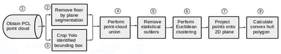
Figure 4.
Point cloud processing pipeline for isolating and determining the location of a general object.
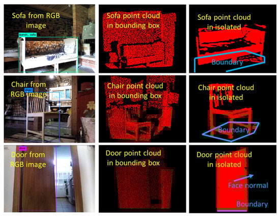
Figure 5.
Point cloud isolation and boundary detection for identified objects.
The PCL pipeline for the isolation and localization of doors is depicted in Figure 6. The first six steps for the PCL pipeline for door recognition are identical to the pipeline for general objects shown in Figure 4. The difference between doors and general objects occurs in Steps 7 and 8. Unlike non-door objects that used a 2D projection and convex hull calculation, door objects used principal components analysis (PCA) in order to determine the object major axes. PCA is an eigen-analysis-based technique [49]. With the principal (eigen) components known, an oriented bounding box (OBB) is placed around the object. The choice of an OBB rather than an axis-aligned bounding box (AABB) was made since the principal axes of the furniture do not always align with the global basis vectors. Due to their long and planar shape, doors lend themselves to accurate PCA and orientation within a bounding box. The bounding box provides the best shape to determine the door’s current position.
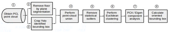
Figure 6.
PCL pipeline for isolating and determining the location of a door.
The door location-determination algorithm is outlined in pseudo code from lines 9 to 25 in Figure 7. For each door that is identified, a bounding box is determined, and the 3D semantic model is searched for a door axis that fits within this box. If such an axis is found, the possible door positions are iterated over from the least extent (door closed) to the maximum extent (door wide open) with a fixed interval of π/20 (meaning that 20 possible door positions are searched for a door that can be opened 180°, or 10 positions for a door that can be opened to at most right angles). A normal vector is calculated for each door position, and it is compared to planes that have been found within the point-cloud. When a match is found, the location of the door has been identified accurately.
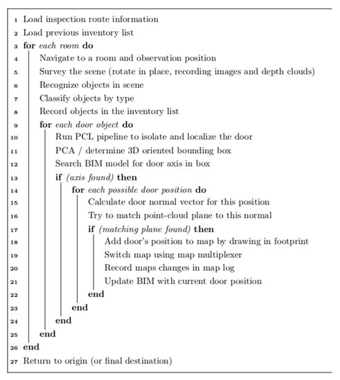
Figure 7.
Pseudo code identifying doors and insertion into navigation map and BIM.
4.6. Real-Time Map Update and Localization
After detecting various types of objects and determining their locations and boundaries, the results are updated on the 2D map to reflect the current state of the environment during navigation. Due to different impacts on robot navigation, this study maintains a dictionary of objects that groups commonly observed objects into two categories that are long-term objects and transient objects. Long-term objects include objects, such as sofas, doors, and refrigerators, which do not frequently move and confuse the traditional navigation approaches. On the other hand, transient objects are objects, such as humans, which dynamically move frequently but not significantly impact navigation due to their shapes. This study updates geometric information of only long-term objects as their presences can significantly impact navigation for a prolonged period. Transient objects are not directly updated in the navigation map, as commonly used AMCL navigation can avoid objects, such moving persons, while changing navigation routes. The benefit of updating the map with human locations is minimal because their presences do not confuse localization and navigation, such as long-term objects with large surfaces. Though this study presents one case of categorizing objects in common indoor buildings, different ways of object categorization can be suggested for navigations in different types of buildings to utilize semantic information for navigation.
In order to perform this task within the software framework, a dedicated, self-contained ROS node was written in C++. This node listens for and acts on messages sent by the object detection and localization routine described in the section above. When an object is detected, the node classifies that node based on the type of object recognized. For long-term objects, the node was designed to automatically insert all such objects directly into the navigation map, whereas a more nuanced version of classification is foreseen for more complicated situations, perhaps using behavior-trees or other higher-level decision capabilities. Transient objects, such as humans, were also identified by the image-recognition software. A classification dictionary is used to determine what action should be taken for each identified object. Because humans are transient, they were determined not to belong as non-structural permanent objects within the navigation map. Each classified long-term object was also saved within a file of identified objects. This file can be used to repopulate an original map from a previous state or simply as a record of all objects identified. Detected objects belong within the navigation map so that at the outset of each surveillance routine, the most up-to-date information is available for route planning, navigation, and localization. The map is continually updated, meaning objects are added and maintained within the map. The entire object is reduced to a 2D footprint represented as a convex hull polygon, as described in the previous section. This convex hull is localized within the coordinate frame of the structure and matched to that of the maps. The map coordinates are iterated over from the upper-left corner to lower-right. Each point (representing a 2D coordinate) is compared to the convex hull to determine if it resides within or outside of the hull. If it resides within the hull, the map point is over-written with a black pixel to indicate that this space is filled, as per the PGM map specification [50]. Alternatively, lighter grey could be used to indicate that this space is not part of the permanent structure so long as the darkness intensity of the pixel is high enough to exceed the threshold for the AMCL navigation routine’s value for a filled point. In order to increase the speed of checking each point for inclusion in the convex hull, a simple x–y axis-aligned bounding box is used to quickly rule out all points of the PGM map that could not fall within the hull since they do not fall within the enclosing AABB. This greatly reduces the number of points that need to be checked for the more computationally intensive task of inclusion in the convex hull. Similarly, current door positions are marked within the navigation. However, door positions will change often, perhaps even during a single surveillance task. Therefore, door positions are recorded in their own file, which can be quickly updated. When a door position is updated, the base map is copied from the most recently updated map containing long-term objects, and then, each door is added using the last known door position. In this way, long-term objects, such as furniture and appliances, remain in their place, and doors are able to change position frequently. After the new map has been copied and modified, it is made immediately available within the ROS ecosystem (e.g., for use by the navigation system) by spawning a new map server node. In order to avoid naming conflicts, each map server is set to broadcast on its own map topic name. A relay node is used to determine the map server that should broadcast to the principal/map topic. This process is illustrated in Figure 8, in which an initial map without a sofa is used for navigation. After the robot identifies and classifies the sofa, it is inserted into the PGM map, which is then served to the navigation system.
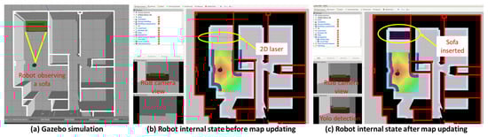
Figure 8.
Example of object recognition and navigation map updating. (a) Robot observing a sofa in a Gazebo simulation, (b) robot’s internal state before map updating, and (c) robot’s internal state after map updating.
5. Case Studies: Localization in a Real-World Indoor Environment
In this section, we present two case studies performed to demonstrate how the accuracy and robustness of indoor robot localization can be enhanced by allowing a mobile robot to recognize non-structural elements and update the map during the navigation. Case studies were conducted in a furnished apartment (Figure 9a) using a mobile robot called Turtlebot2 (Figure 9b). Based on the Kobuki mobile base, an Orbbec Astra camera and Slamtec RPLidar were installed for object recognition and localization, respectively. The Orbbec Astra camera collects sensor messages including RGB image, depth images, and the point cloud, which are required as input for YOLO-based object recognition and point cloud processing. The Slamtect RPLidar collects 360-degree 2D LiDAR scans that are required to match the current location with locations in the 2D AMCL map. The living space is a 100 m2 (1076 ft2) residential apartment that contains floors made of wood and marble. The doors in the apartment are mostly single doors with an average width of 71 cm (28 in). These widths, along with the hallway widths, are large enough for the TurtleBot2 to navigate without any issue. There is one set of double doors separating the dining and foyer areas, which is used for a portion of the case study.
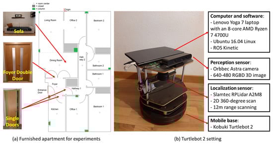
Figure 9.
(a) Furnished apartment for experiment and (b) Turtlebot2 with RGBD and 2D LiDAR sensors.
The case studies included both traditional localization (case study 1) and kidnapped robot (case study 2) scenarios. At the beginning of case study 1, as shown in Figure 10a, the robot first navigated the apartment along a predefined path from station 1 to station 10 and updated the original unaltered map with objects recognized by the Astra RGBD camera. By performing map updating, the robot was expected to correct errors caused by non-structural elements and adjust its XY location and orientation automatically. Then, we compared how the accuracy was impacted when the robot without map-updating capability utilized the unaltered original map as the present state-of-practice. Similarly, in case study 2, we compared the time and accuracy of localization when different maps (original unaltered map and the map updated from case study 1) were used in kidnapped robot situations. As shown in Figure 10b, the robot was carried to arbitrary locations (five stations) by a human. Even though the initial belief about the current pose was in office 2, the robot was instructed to rotate at its unknown locations to recover the current pose by matching the 2D LiDAR scans with the given maps. In these two case studies, the types of non-building objects were limited to doors and sofa. However, other common items can be included in practical implementations. One important aspect when considering localization is parameter setting to configure the AMCL algorithm. As shown in Table 1, the values of the AMCL parameters were set differently for traditional localization and kidnapped robot scenarios. For the kidnapped robot, a larger number of particles was generated (min_particle and max_particles), spread farther from the arbitrary location (init_cov_xx, init_cov_yy, and init_cov_aa), and converged slower (resample_interval, recovery_alpha_slow, and recovery_alpha_fast) to explore and search potential locations all over the building.
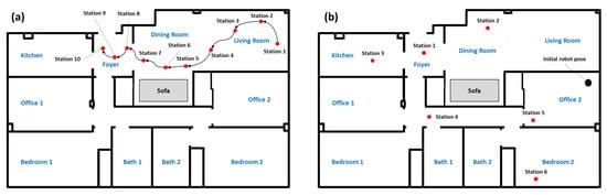
Figure 10.
(a) Navigation path for traditional localization and (b) robot locations for kidnapped localization.

Table 1.
Modifications to the AMCL default parameters for the kidnapped robot problem.
5.1. Case Study 1: Traditional Localization Scenario
Case study 1 started with the Turtlebot2 navigating the indoor environment while updating the map. The robot started from a known, accurate location (station 1) using the unaltered map with walls of the apartment, without furniture or doors. As shown in Figure 11, the robot was instructed to visit ten stations in living room, dining room, and foyer area while updating the map when non-structural objects (e.g., sofa or doors) were detected by the Astra camera. During the map updating, localization errors were corrected automatically. Then, in another experiment for comparison, the robot was instructed to repeat navigation of the path without using the object recognition and map updating as the state-of-practice. This provided a demonstration of the difference between employing the software versus the current method. Each scenario was repeated three times. Figure 11 shows how the map was updated during the navigation. Around station 5, the robot identified the presence of a couch with the camera, isolated its point cloud from the depth cloud, and inserted the 2D boundary polygon into the map. At station 7 around the foyer, the robot detected a set of double-doors and updated the map. Finally, at the final location in the foyer, the robot rotated around to detect and update three more doors.
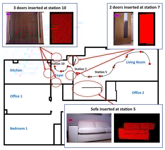
Figure 11.
Robot navigation along a given path with object recognition and map updating.
As shown in Table 2, the accuracy of localization with map updating implemented was highly reliable, with location errors within 10 cm and orientation errors of 0.1 radian (about 6 degrees). However, localization without map updating suffered from non-building elements existing around the path. The localization for the initial part without non-building elements was highly accurate (station 1–4). However, once the robot approached the couch, the error started increasing with the robot interpreting the front of the sofa as the wall behind it (station 5–7). This led to the robot “jumping” by roughly one meter towards the direction of the wall at station 7. Then, as the robot entered the foyer area, closed doors (three single doors and one of double doors) made the 2D shape of the foyer area similar to rooms without doors, eventually determining the location to be bathroom 1. At this point, the robot could not recover its location and could not proceed to station 8–10. Figure 12 shows how the AMCL particle swarms evolved during the navigation. With map updating, the robot could arrive at station 10 automatically recovering from errors. However, without map updating, the robot could not recover location and orientation errors caused by the sofa around station 5 and 6, which then accumulated around 7 to jump to a location far from the final destination.
Table 2.
Results of one trial of the traditional localization experiment (values are in meters and radians).
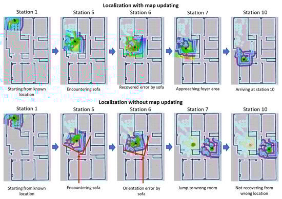
Figure 12.
Traditional localization scenario: navigation without map updating (top) and traditional navigation with map updating (bottom).
5.2. Case Study 2: Kidnapped Robot Scenario
Kidnapped robot tests were performed to evaluate how fast and accurately a robot can determine its position in the map when the robot was moved to arbitrary locations. As shown in Figure 10b, six stations were selected for different kidnapped positions. The initial pose represents the initial belief about the current pose from which the robot should recover. For station 1 in a foyer area, a set of sub-tests was performed because there are multiple possible states due to six doors that can be either correctly or incorrectly represented in the map. The doors were either fully open or closed in real life, and the map was altered to show the doors being fully open or closed. At station 1, the robot was placed in the center of the foyer and rotated until it could localize itself. If a full minute of rotation was undertaken without the robot being able to locate itself, the experiment was stopped and marked as a failure. For each case, a total of five identical iterations of the experiment was performed. Each of the cases resulted in the robot being able to localize itself after rotating multiple times. The average time and standard deviations for each iteration are given in Table 3. As shown in the results, all kidnapped robot positioning-utilizing maps accurately presenting the actual door states successfully determined the current positions, and the location error ranged from 2 cm to 8 cm, averaging 5 cm, for all successful localizations. For example, in the case where the map showed all doors open, the robot failed to locate itself regardless of the actual door configurations. However, for each case where the map matched the real-life door configuration, the robot was able to localize itself within the 60 s cut-off. While some of the localization trials were faster for maps that did not match the door layout, localization was more successful and fastest when the maps matched reality. Figure 13 shows how the AMCL particle swarms evolve during rotation searching for the best match between the map and 2D LiDAR scans. Due to the AMCL setting in Table 1, the initial swarm was spread in a wide area around the initial belief. Then, the swarm converged to the most likely positions making the robot jump to different locations. While the robot was able to accurately determine the location when it used an accurate map, a wrong location was determined after four rotations when it used a map with inaccurate door states. The robot’s position could not recover from the incorrect localization regardless of many rotations were made.
Table 3.
Results of the kidnapped robot in station 1 with different door configurations.
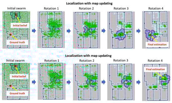
Figure 13.
Evolution of particle swarms for actual door configuration OOOOXO using an accurate map (OOOOXO) and inaccurate map (OOOOOO).
All adjacent doors were closed for the remainder of the kidnapped localization at stations 2–6. A comparison of the average time necessary for localization using the updated map versus the original map was undertaken, with the results being presented in Table 4. Error ranged from 2 cm to 8 cm, averaging 5 cm, for all successful localizations. All of the scenarios relying on the original map failed in localization, except for station 6. This is likely due to the simple rectangular rooms that do not provide enough geometric differentiation for the AMCL algorithm to correctly localize it if it is rotating in one place. This was also found to be the case even if an updated map was used for stations 3 and 5. Station 4 took a significant number of rotations before it converged to the correct location. Unlike that with traditional localization, the results of kidnapped robot scenarios show that the map updating could provide limited aids in localization in these challenging conditions.
Table 4.
Results of localization at stations 2–6, with the average time in seconds before accurate localization.
6. Conclusions and Discussion
Accurate localization is an essential component in developing a robot-based processes in a built environment. Creating and updating a map of the environment plays an important role in accurately estimating its own location. However, most of the conventional robot localization methods have grounded their approaches on an assumption that the environments are static without considerations about non-structural elements not presented in the map negatively impacting the accuracy and robustness of localization. In order to address this limitation, our study proposed an AMCL-based indoor robot localization method, improved in terms of accuracy and robustness, which comprises combined object recognition and semantic three-dimensional building map dynamical updating. In this approach, (1) A 2D map generated based on BIM is provided to the mobile robot, and it navigates it with the SLAM algorithm using that information, (2) a mobile robot moves around an indoor environment to collect 3D point cloud data with a depth camera and extracts semantic object information that has not existed in the BIM model, and (3) the extracted new object information is updated and reflected in the two-dimensional map so that it can be used to improve the accuracy of localization and possibly for path planning, mission planning, and construction management process. By performing case studies with both traditional localization and kidnapped robot scenarios, this study proved that the map-updating capability embedded in AMCL localization could enhance the accuracy and robustness of a mobile robot’s indoor localization. In the given environment, a mobile robot could accurately update a map of the indoor environment with non-structural objects using sensors, and importantly, by utilizing a continuously updated indoor map, accuracy and robustness could be enhanced in both traditional navigation and kidnapped localization scenarios. Moreover, by performing localization without map updating, this study found that indoor localization is significantly impacted by how non-structural elements are presented in a robot’s map for the operating environment. Our study is distinguishable from existing approaches mainly because of the capability to detect non-structural elements during localization. We present a new process that detects non-structural elements with sensors and incorporates them into a semantic building map. Unlike conventional metric maps, the semantic 3D map of the building allows for a precise presentation of elements with their parameters (such as doors) instead of simple 2D shapes. From the 3D map, we directly generated 2D metric maps that are inputted for AMCL-based localization. By updating the maps in real-time, our approach allowed the robot to correct errors caused by non-structural elements without input from human users.
However, there are several limitations that will lead to future studies. During the map updating, only the front boundaries of the objects were detected and inserted into the map. Even though this allowed for the real-time correction of localization errors, the estimation of exact poses of the elements was not achieved in this project. In future studies, exact poses of various types of elements can be calculated by preparing an inventory of elements in the environment. A 3D point cloud of the detected object can be aligned to point cloud templates of objects in the inventory so that the robot can fully understand the states of the elements with partial observations. The information about these non-structural elements can then be incorporated into a BIM model of the environment for various purposes, including building asset management, inventory checking, and occupancy monitoring. Moreover, our study did not overcome the reliance on 2D laser scans, which is a fundamental limitation of AMCL localization. Since the 2D laser scan inspects 2D features at a certain height, the performance can be greatly impacted by slight changes in the environment. Future studies can create a 3D point cloud of the environment using SLAM and overlay it on the semantic building model to achieve greater accuracy and resiliency to changes in the environment. Finally, for practical implementation of the proposed approach, various other non-structural elements should be included in the scope of object detection. The list of elements can vary depending on the types of buildings. For example, desks, tables, chairs, students, and monitors can be included as commonly observed elements for implementation in educational facilities.
Author Contributions
Conceptualization, K.K.; methodology, M.P. and K.K.; software, M.P. and K.K.; validation, M.P. and K.K.; formal analysis, M.P.; writing—original draft preparation, M.P. and K.K.; writing—review and editing, P.K. and H.O.; All authors have read and agreed to the published version of the manuscript.
Funding
This research received no external funding.
Informed Consent Statement
Not applicable.
Data Availability Statement
Data is unavailable due to privacy.
Conflicts of Interest
The authors declare no conflict of interest.
References
- Huang, S.; Dissanayake, G. Robot Localization: An Introduction. In Wiley Encyclopedia Electrical and Electronics Engineering; John Wiley & Sons, Inc.: Hoboken, NJ, USA, 1999; pp. 1–10. [Google Scholar]
- Liu, H.; Zheng, X.; Sun, F. Orientation Estimate of Indoor Mobile Robot Using Laser Scans. J. Tsinghua Univ. Sci. Technol. 2018, 58, 609–613. [Google Scholar]
- Dobrev, Y.; Flores, S.; Vossiek, M. Multi-Modal Sensor Fusion for Indoor Mobile Robot Pose Estimation. In Proceedings of the IEEE/ION PLANS 2016, Savannah, GA, USA, 11–14 April 2016; pp. 553–556. [Google Scholar]
- Eman, A.; Ramdane, H. Mobile Robot Localization Using Extended Kalman Filter. In Proceedings of the 2020 3rd International Conference on Computer Applications & Information Security (ICCAIS), Riyadh, Saudi Arabia, 19–21 March 2020; pp. 1–5. [Google Scholar]
- Raghavan, A.N.; Ananthapadmanaban, H.; Sivamurugan, M.S.; Ravindran, B. Accurate Mobile Robot Localization in Indoor Environments Using Bluetooth. In Proceedings of the 2010 IEEE International Conference on Robotics and Automation, Anchorage, AK, USA, 3–7 May 2010; pp. 4391–4396. [Google Scholar]
- Tao, B.; Wu, H.; Gong, Z.; Yin, Z.; Ding, H. An RFID-Based Mobile Robot Localization Method Combining Phase Difference and Readability. IEEE Trans. Autom. Sci. Eng. 2020, 18, 1406–1416. [Google Scholar] [CrossRef]
- Nazemzadeh, P.; Fontanelli, D.; Macii, D.; Palopoli, L. Indoor Localization of Mobile Robots through QR Code Detection and Dead Reckoning Data Fusion. IEEE/ASME Trans. Mechatron. 2017, 22, 2588–2599. [Google Scholar] [CrossRef]
- Luan, J.; Zhang, R.; Zhang, B.; Cui, L. An Improved Monte Carlo Localization Algorithm for Mobile Wireless Sensor Networks. In Proceedings of the 2014 Seventh International Symposium on Computational Intelligence and Design, Washington, DC, USA, 13–14 December 2014; Volume 1, pp. 477–480. [Google Scholar]
- Dellaert, F.; Fox, D.; Burgard, W.; Thrun, S. Monte Carlo Localization for Mobile Robots. In Proceedings of the 1999 IEEE International Conference on Robotics and Automation (Cat. No. 99CH36288C), Detroit, MI, USA, 10–15 May 1999; Volume 2, pp. 1322–1328. [Google Scholar]
- Quigley, M.; Conley, K.; Gerkey, B.; Faust, J.; Foote, T.; Leibs, J.; Wheeler, R.; Ng, A.Y. ROS: An Open-Source Robot Operating System. In Proceedings of the ICRA Workshop on Open Source Software, Kobe, Japan, 12–17 May 2009; Volume 3, p. 5. [Google Scholar]
- ROS.org Amcl—ROS Wiki. Available online: http://wiki.ros.org/amcl (accessed on 13 July 2021).
- Stahl, T.; Wischnewski, A.; Betz, J.; Lienkamp, M. ROS-Based Localization of a Race Vehicle at High-Speed Using LIDAR. In Proceedings of the E3S Web of Conferences, Prague, Czech Republic, 16–19 February 2019; Volume 95, p. 4002. [Google Scholar]
- Dos Reis, W.P.N.; Morandin, O.; Vivaldini, K.C.T. A Quantitative Study of Tuning ROS Adaptive Monte Carlo Localization Parameters and Their Effect on an AGV Localization. In Proceedings of the 2019 19th International Conference on Advanced Robotics (ICAR), Belo Horizonte, Brazil, 2–6 December 2019; pp. 302–307. [Google Scholar]
- Panchpor, A.A.; Shue, S.; Conrad, J.M. A Survey of Methods for Mobile Robot Localization and Mapping in Dynamic Indoor Environments. In Proceedings of the 2018 Conference on Signal Processing and Communication Engineering Systems (SPACES), Vijayawada, India, 4–5 January 2018; pp. 138–144. [Google Scholar]
- Gao, X.; Li, J.; Fan, L.; Zhou, Q.; Yin, K.; Wang, J.; Song, C.; Huang, L.; Wang, Z. Review of Wheeled Mobile Robots’ Navigation Problems and Application Prospects in Agriculture. IEEE Access 2018, 6, 49248–49268. [Google Scholar] [CrossRef]
- Alatise, M.B.; Hancke, G.P. Pose Estimation of a Mobile Robot Based on Fusion of IMU Data and Vision Data Using an Extended Kalman Filter. Sensors 2017, 17, 2164. [Google Scholar] [CrossRef] [PubMed]
- Sasiadek, J.Z.; Hartana, P. Sensor Fusion for Dead-Reckoning Mobile Robot Navigation. IFAC Proc. Vol. 2001, 34, 251–256. [Google Scholar] [CrossRef]
- Park, K.; Chung, H.; Lee, J.G. Dead Reckoning Navigation for Autonomous Mobile Robots. IFAC Proc. Vol. 1998, 31, 219–224. [Google Scholar] [CrossRef]
- Lizarralde, F.; Nunes, E.V.L.; Hsu, L.; Wen, J.T. Mobile Robot Navigation Using Sensor Fusion. In Proceedings of the 2003 IEEE International Conference on Robotics and Automation (Cat. No. 03CH37422), Taipei, Taiwan, 14–19 September 2003; Volume 1, pp. 458–463. [Google Scholar]
- Fan, B.; Li, Q.; Liu, T. How Magnetic Disturbance Influences the Attitude and Heading in Magnetic and Inertial Sensor-Based Orientation Estimation. Sensors 2017, 18, 76. [Google Scholar] [CrossRef]
- Patle, B.K.; Pandey, A.; Parhi, D.R.K.; Jagadeesh, A. A Review: On Path Planning Strategies for Navigation of Mobile Robot. Def. Technol. 2019, 15, 582–606. [Google Scholar] [CrossRef]
- Almasri, M.; Elleithy, K.; Alajlan, A. Sensor Fusion Based Model for Collision Free Mobile Robot Navigation. Sensors 2015, 16, 24. [Google Scholar] [CrossRef]
- Jeon, D.; Choi, H.; Kim, J. UKF Data Fusion of Odometry and Magnetic Sensor for a Precise Indoor Localization System of an Autonomous Vehicle. In Proceedings of the 2016 13th International Conference on Ubiquitous Robots and Ambient Intelligence (URAI), Xi’an, China, 19–22 August 2016; pp. 47–52. [Google Scholar]
- Debeunne, C.; Vivet, D. A Review of Visual-LiDAR Fusion Based Simultaneous Localization and Mapping. Sensors 2020, 20, 2068. [Google Scholar] [CrossRef]
- Behzadian, B.; Agarwal, P.; Burgard, W.; Tipaldi, G.D. Monte Carlo Localization in Hand-Drawn Maps. In Proceedings of the 2015 IEEE/RSJ International Conference on Intelligent Robots and Systems (IROS), Hamburg, Germany, 28 September–2 October 2015; pp. 4291–4296. [Google Scholar]
- Feng, Q.; Cai, H.; Li, F.; Liu, X.; Liu, S.; Xu, J. An Improved Particle Swarm Optimization Method for Locating Time-Varying Indoor Particle Sources. Build Environ. 2019, 147, 146–157. [Google Scholar] [CrossRef] [PubMed]
- Biswas, J.; Veloso, M. Episodic Non-Markov Localization: Reasoning about Short-Term and Long-Term Features. In Proceedings of the 2014 IEEE International Conference on Robotics and Automation (ICRA), Hong Kong, China, 31 May–7 June 2014; pp. 3969–3974. [Google Scholar]
- Ferguson, M.; Jeong, S.; Law, K.H. Worksite Object Characterization for Automatically Updating Building Information Models. In Proceedings of the Computing in Civil Engineering 2019, Atlanta, GA, USA, 17–19 June 2019; American Society of Civil Engineers: Reston, VA, USA; pp. 303–311. [Google Scholar]
- Correa, F. Robot-Oriented Design for Production in the Context of Building Information Modeling. In Proceedings of the ISARC—The International Symposium on Automation and Robotics in Construction, Auburn, AL, USA, 18–21 July 2016; Volume 33, p. 1. [Google Scholar]
- Thrun, S.; Fox, D.; Burgard, W. Probabilistic Mapping of an Environment by a Mobile Robot. In Proceedings of the 1998 IEEE International Conference on Robotics and Automation (Cat. No.98CH36146), Leuven, Belgium, 20 May 1998; Volume 2, pp. 1546–1551. [Google Scholar]
- Choset, H.; Nagatani, K. Topological Simultaneous Localization and Mapping (SLAM): Toward Exact Localization without Explicit Localization. IEEE Trans. Robot. Autom. 2001, 17, 125–137. [Google Scholar] [CrossRef]
- Kuric, I.; Bulej, V.; Saga, M.; Pokorny, P. Development of Simulation Software for Mobile Robot Path Planning within Multilayer Map System Based on Metric and Topological Maps. Int. J. Adv. Robot. Syst. 2017, 14, 1–14. [Google Scholar] [CrossRef]
- Konolige, K.; Bowman, J.; Chen, J.D.; Mihelich, P.; Calonder, M.; Lepetit, V.; Fua, P. View-Based Maps. Int. J. Rob. Res. 2010, 29, 941–957. [Google Scholar] [CrossRef]
- Labbe, M.; Michaud, F. Appearance-Based Loop Closure Detection for Online Large-Scale and Long-Term Operation. IEEE Trans. Robot. 2013, 29, 734–745. [Google Scholar] [CrossRef]
- Labbe, M.; Michaud, F. Online Global Loop Closure Detection for Large-Scale Multi-Session Graph-Based SLAM. In Proceedings of the 2014 IEEE/RSJ International Conference on Intelligent Robots and Systems, Chicago, IL, USA, 14–18 September 2014; pp. 2661–2666. [Google Scholar]
- Galindo, C.; Saffiotti, A.; Coradeschi, S.; Buschka, P.; Fernandez-Madrigal, J.A.; Gonzalez, J. Multi-Hierarchical Semantic Maps for Mobile Robotics. In Proceedings of the 2005 IEEE/RSJ International Conference on Intelligent Robots and Systems, Edmonton, AB, Canada, 2–6 August 2005; pp. 2278–2283. [Google Scholar]
- Galindo, C.; Fernández-Madrigal, J.A.; González, J.; Saffiotti, A. Robot Task Planning Using Semantic Maps. Robot. Auton. Syst. 2008, 56, 955–966. [Google Scholar] [CrossRef]
- Vasudevan, S.; Siegwart, R. Bayesian Space Conceptualization and Place Classification for Semantic Maps in Mobile Robotics. Robot. Auton. Syst. 2008, 56, 522–537. [Google Scholar] [CrossRef]
- Nüchter, A.; Hertzberg, J. Towards Semantic Maps for Mobile Robots. Robot. Auton. Syst. 2008, 56, 915–926. [Google Scholar] [CrossRef]
- Ranganathan, A.; Dellaert, F. Semantic Modeling of Places Using Objects. In Proceedings of the Robotics: Science and Systems III, Atlanta, GA, USA, 27–30 June 2007; Robotics: Science and Systems Foundation: Atlanta, GA, USA, 2007. [Google Scholar]
- Kruijff, G.-J.M.; Zender, H.; Jensfelt, P.; Christensen, H.I. Situated Dialogue and Spatial Organization: What, Where… and Why? Int. J. Adv. Robot. Syst. 2007, 4, 16. [Google Scholar] [CrossRef]
- Kim, S.; Peavy, M.; Huang, P.-C.; Kim, K. Development of BIM-Integrated Construction Robot Task Planning and Simulation System. Autom. Constr. 2021, 127, 103720. [Google Scholar] [CrossRef]
- Kim, K.; Peavy, M. BIM-Based Semantic Building World Modeling for Robot Task Planning and Execution in Built Environments. Autom. Constr. 2022, 138, 104247. [Google Scholar] [CrossRef]
- Bochkovskiy, A.; Wang, C.-Y.; Liao, H.-Y.M. YOLOv4: Optimal Speed and Accuracy of Object Detection. arXiv 2020, arXiv:2004.10934. [Google Scholar]
- Arduengo, M.; Torras, C.; Sentis, L. Robust and Adaptive Door Operation with a Mobile Robot. Intell. Serv. Robot. 2021, 14, 409–425. [Google Scholar] [CrossRef]
- Google Research Google Colaboratory. Available online: https://research.google.com/colaboratory (accessed on 29 November 2021).
- Point Cloud Library Plane Model Segmentation. Available online: https://pcl.readthedocs.io/en/latest/planar_segmentation.html (accessed on 20 March 2022).
- Point Cloud Library Euclidean Cluster Extraction. Available online: https://pcl.readthedocs.io/en/latest/cluster_extraction.html (accessed on 20 March 2022).
- Champion, K.; Lusch, B.; Kutz, J.N.; Brunton, S.L. Data-Driven Discovery of Coordinates and Governing Equations. Proc. Natl. Acad. Sci. USA 2019, 116, 22445–22451. [Google Scholar] [CrossRef] [PubMed]
- Yang, H. GitHub—Pgm_map_creator: Create Pgm Map from Gazebo World File for ROS Localization. Available online: https://github.com/hyfan1116/pgm_map_creator (accessed on 29 November 2021).


Disclaimer/Publisher’s Note: The statements, opinions and data contained in all publications are solely those of the individual author(s) and contributor(s) and not of MDPI and/or the editor(s). MDPI and/or the editor(s) disclaim responsibility for any injury to people or property resulting from any ideas, methods, instructions or products referred to in the content. |
© 2023 by the authors. Licensee MDPI, Basel, Switzerland. This article is an open access article distributed under the terms and conditions of the Creative Commons Attribution (CC BY) license (https://creativecommons.org/licenses/by/4.0/).