1. Introduction
With the progress of wireless communication technology and information technology and the continuous emergence of various sensing devices, intelligent vehicles equipped with wireless communication units, computing equipment, electronic maps and a large number of sensors appear. With the help of On Board Units (OBUs), intelligent vehicles constitute the Internet of Vehicles (IoV). As the most potential industrial application in the fields of 5G, transportation and automobile, IoV is an important part of the future intelligent transportation system [
1,
2]. However, rogue nodes (bad nodes), which spread false information or malicious information in the network, bring many problems to the entire network, such as high network delay, data inconsistency and data loss. These problems have a great impact on the actual traffic environment, resulting in traffic jams, vehicle collisions, etc., which bring social losses. Hence, rogue node discovery plays an important role in building a secure IoV environment.
Previous research proposed machine learning-based methods to detect rogue nodes [
3,
4,
5,
6]. In these works, Support Vector Machine classifiers (SVM), K-Nearest Neighbor (KNN), Random Forest (RF) algorithm, etc., are used for rogue vehicle detection. These above methods can identify a certain number of rogue nodes. However, they rely too much on historical data. Further, these methods may lead to long network delay and slow detection speed [
6]. Since using the computing power of roadside units (RSUs) can obtain more accurate detection results, studies [
7,
8,
9] proposed to use the RSUs deployed on the road to discover the rogue node. However, both the number and the coverage of the RSUs in the urban area are limited. Therefore, it is difficult to obtain real-time detection when the traffic load is heavy. Moreover, RSU-based rogue vehicle detection strategies cannot work if the RSUs become failed due to disasters. To discover rogue vehicles, Paranjothi et al. [
10] proposed to dynamically create a fog network composed of moving vehicles in the detection area. However, due to the fast speed of moving vehicles, the stability of the fog network is difficult to guarantee.
Based on the widespread parked vehicles in cities, this paper proposes a rogue node detection scheme based on roadside parked vehicles. In this paper, parked vehicles on a road automatically form parking clusters at first. Then, a prediction model is built to predict the vehicles that will continue to stay in the cluster in the next few hours. A fog network composed of stable parked vehicles is dynamically established. Finally, a U-test method based on hypothesis testing is proposed in order to detect rogue vehicles. To achieve fast and efficient rogue vehicle detection, we let all nodes in the fog network perform rogue node detection in parallel. Simulation results show that the proposed scheme has higher detection accuracy and stability than other rogue node detection schemes. We summarize our contributions as follows:
(1) We propose a parked vehicle stability prediction model to predict the probability that the parked vehicle will continue to stay in the cluster in the future period of time. Stable vehicles are then selected to form a fog network, in which fog nodes cooperate with each other to detect rogue nodes to reduce the delay of bad node discovery. Since the formed fog network is stable, the calculation migration overhead caused by the leaving of the fog node is avoided. To the best of our knowledge, this is the first attempt that tries to decrease the processing delay of bad nodes by using parked vehicles in cities.
(2) To adapt to the dynamic changes of traffic conditions, we let the number of fog nodes correspond to the moving vehicle density on the road. To obtain the density of moving vehicle on the road, the Greenshield model is used to model the current road conditions.
(3) To detect rogue nodes effectively, a machine learning method is firstly used to classify the moving vehicles according to the average moving speed of the vehicle. Then, a novel U-test rogue node detection method, which is performed by fog nodes, is proposed to further discover the bad nodes.
2. Related Work
The detection of rogue nodes can be roughly divided into two categories: the first category is the use of machine learning methods to identify rogue nodes, and the second one is the use of non-machine learning strategies for rogue node detection. Kang, M.J. [
11] proposed an intrusion detection system based on a deep belief network, which used unsupervised pre-training to initialize parameters, thus improving the detection accuracy. Fei Li [
12] proposed an intrusion detection system based on VANETs, which used a self-encoder network and a recurrent neural network to achieve efficient intrusion detection. The methods proposed in [
11,
12] have the problem that the generalization ability of the model is not strong due to the large difference between the training data set and the actual application. Literature [
3] proposed a scheme based on SVM to defend against false information. The local trust module used the SVM-based classifier to detect false messages, and the vehicle trust module applied SVM to obtain the comprehensive trust value of the vehicle. Rogue nodes can be determined by combining the detection results of the two types of modules. However, this method has the problem of over-reliance on historical data, resulting in low recognition accuracy. Research [
4] used an SVM-based module to analyze historical vehicle data to calculate the vehicle’s trust value, which was then used to detect rogue nodes. However, this mechanism showed high network latency and storage overhead when the density of automobiles in the city was high. Zang et al. [
5] proposed an intrusion detection algorithm based on machine learning to monitor network traffic and detect abnormal network activities. However, due to the lack of samples, this algorithm had low universality for different network abnormal behavior detection. Ercan et al. [
6] used KNN and RF to establish a generalized detection mechanism. Although these proposed mechanisms can detect rogue nodes in different scenarios, the detection speed is slow. Further, no response mechanism is established to deal with the detected anomalies.
Nowadays, various non-machine learning-based detection strategies have been proposed. For instance, Liu, J. [
13] proposed a secure intelligent traffic light control scheme based on fog computing. The system used roadside traffic lights as fog equipment, and its security was based on the hardness of the computational Diffie–Hellman puzzle. K. Zaidi [
14] proposed an Intrusion Detection System using statistical techniques to detect anomalies and identify rogue nodes. Paranjothi [
15] proposed a fog computing-based Sybil attack detection for VANETs, which utilized onboard units of all the vehicles in the region to create a dynamic fog for rogue nodes detection. Arif [
16] proposed a VANETs architecture for secure communication, which included two parts: the software defined network and the fog computing. In the interim, fog computing was used to provide secure communication of information. The methods proposed in [
13,
14,
15,
16] have the problem that their performance will generally decline as the number of rogue nodes increases. Ahmed [
7] presented a trust-based approach to classify moving vehicles. The authors used RSUs to calculate the trust score for each vehicle at first. Then, vehicles were classified according to their trust values. To resolve both the information security and the data privacy issues in fog computing, Otaibi et al. [
8] proposed a rogue node detection scheme based on symmetric keys. RSUs first encrypted the rogue node calculation results, and then shared the detection results with other RSUs in the network. The authors in [
9] showed a method that can discover bad nodes based on a group of user equipment. Simulation results presented that the proposed method achieves high performance with minimum implementation overhead. In literature [
10], the authors described the concept of guard nodes for judging illegal nodes. Moving vehicles on the road are employed to form a fog network. A guard vehicle is then chosen by jointly combining the position and the speed of the vehicles in the fog network. The guarding vehicle was responsible for running the corresponding algorithm with the aim of high-accuracy bad node discovery. However, this strategy relied too much on the guard node, which is a bottleneck of the fog network. In addition, the stability of the fog network formed by the moving vehicles is difficult to maintain. Further, Ghaleb et al. [
17] introduced a context-aware misbehavior detection model for local detection of false mobility information. However, research works [
8,
17] all depended on the infrastructure in the urban area. The proposed strategies are inefficient when the infrastructure is overloaded. Moreover, these proposed strategies cannot be used when the RSUs are destroyed or failed.
3. Network Model
3.1. Network Architecture
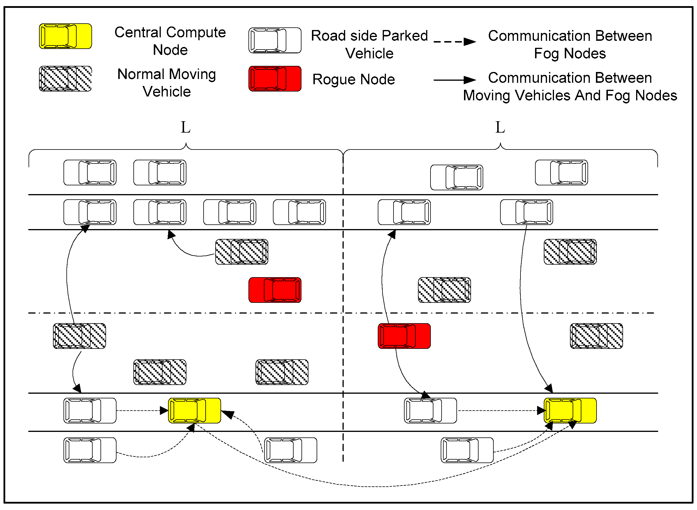
The basic framework of this paper is shown in
Figure 1, which consists of the following three parts: parked vehicles, parking clusters and moving vehicles on the road.
(1) Parked vehicles: Parked vehicles parked on both sides of the roads. Parked vehicles own computation and storage capacities. They are member nodes of the parking clusters.
(2) Parking cluster: It consists of parked vehicles on both sides of the road. A parking cluster includes many cluster members and a cluster head. The cluster head collects cluster member information for maintaining the structure. The cluster head is also responsible for maintaining the historical parking records of parked vehicle members. Moreover, to predict relatively stable parked vehicles in the cluster, a parking prediction model is executed by the cluster head.
(3) Moving vehicle: Moving vehicles are intelligent vehicles driving on the road. Most smart vehicles are equipped with electronic maps, positioning systems, wireless communication modules and various intelligent sensing devices. Moving vehicles can communicate with each other by using the IEEE802.11p protocol [
18].
In this paper, some moving vehicles may be rogue nodes, which need to be detected in time through the formed fog network which is composed of stable parked vehicles in the parking cluster.
3.2. The Construction of Parking Cluster
A parking cluster, which includes some parked vehicle member nodes and a cluster head node, is formed by parked vehicles on both sides of a road. The parking cluster contains sufficient computational capacity. We let the maximum distance between the two endpoint members of a cluster be L meters. In order to reduce the rogue node detection latency, the length of the cluster cannot be too long. Hence, when the road is longer than L meters, the road will be divided into multiple clusters. In each cluster, the parked vehicle that is closest to the center of the cluster is set as the cluster head, and other parked vehicles become cluster members. Each member vehicle periodically sends a notification message to the cluster head to report its ID number, its current location and its remaining power to the head node. The cluster head manages all cluster members and maintains the cluster’ structure. Since the cluster head may drive away, the vehicle adjacent to the cluster head is set as the secondary node, with the aim of improving the reliability of the cluster.
3.3. Parked Vehicle Stability Prediction Model
The proposed parked vehicle stability prediction model in this subsection is executed by the cluster head, with the aim of predicting the parking probability of each member. The parking probability denotes the probability that the vehicle will continue to stay in the cluster in the future period of time. The parked vehicles with higher parking probabilities are selected as fog computing nodes to ensure the relative stability of parked vehicles that will perform fog computing. The data set used here comes from the Jiuzhaigou county government office [
19], which contains parking datasets from 11 March 2020 to 29 March 2020 in the Jiuzhaigou scenic area, Sichuan, China. This data set contains 11 features, as shown in
Table 1. In addition, this data set records the specific time that vehicles enter and exit the parking lot.
Based on this data set, both the number of daily parking times and the average daily parking duration of each vehicle are analyzed.
Figure 2 shows the statistics of the distribution of parking times in each time period within 24 h of a day. As shown in
Figure 2, the number of parking times is the maximum from 8:00 a.m. to 17:00 p.m. of a day, and the peak of the stop of vehicles is around 10:00 a.m. in the morning. The least number of stops are from 4:00 a.m. to 6:00 a.m. in the morning.
Figure 3 shows the average parking duration of the vehicles in the parking lot. It can be seen from this figure that most of the parked vehicles stay in the parking lot for 1 to 8 h, and the number of vehicles that parked for more than 3 h account for 87.8% of the total number of parked vehicles.
Feature extraction is the key to data analysis. Combined with the attribute information of the data set, we select 10,000 pieces of data and extract 6 key attribute features for model analysis. These six features are vehicle code, parking lot ID number, parking order number, historical times of parking, average parking time and the longest parking duration of each parked vehicle. Through the extraction of the above features, the corresponding relationship between each vehicle and each parking lot is sorted out and 2826 new pieces of data is obtained. The first 2000 pieces of data are selected as training data and the rest of the data are test data. The training set is processed by a linear model to raise and then reduce the original four-dimensional data. Finally, one-dimensional data are obtained. In addition, since this problem is a binary classification problem, it needs to be activated by the sigmoid function so that the parking probability is distributed between 0 and 1. The neural network model is shown in
Figure 4, which adopts a fully connected neural network, including an input layer, hidden layers and an output layer. The probability of stable parking of the vehicle is given by the sigmoid function.
Figure 5a denotes the variation of the average entropy loss vs. the training epochs. It can be seen that the cross entropy loss converges around 0.37 after about 1000 epochs.
Figure 5b shows the variation of average prediction accuracy with the varying of training epochs. As can be seen from the figure, the prediction accuracy reaches about 76%, and the average accuracy on the test set is 72.67%. Therefore, we can conclude that whether the vehicle will continue to stay in the cluster in the next several hours can be predicted with a high accuracy by using the proposed prediction model.
3.4. Fog Network Construction
Based on the above-mentioned prediction model, the set of vehicles that will continue to stay in the parking cluster in the next few hours is obtained. The fog nodes should be selected from these candidate parked vehicles. This is because selecting stable parked vehicles as fog computing nodes can avoid the computational migration cost caused by the sudden departure of the cluster member during the rogue node calculation process. At the same time, the number of fog nodes in the fog network should be related to the density of moving vehicles on the road. The higher the density of the moving vehicles, the more fog computing nodes should be needed to speed up the detection of rogue nodes. We select several nodes with high parking probability in the parking cluster to form the fog network. The fog node selection process is described as follows:
(1) Firstly, the Greenshield model [
20] is used to model the density of moving vehicles on the road where the parking cluster is located. The Greenshield model, which is widely used to model uninterrupted traffic conditions, is recognized as a highly accurate traffic flow statistical model in the field of traffic engineering. In the Greenshield model, vehicle density is inversely proportional to vehicle speed, and an increase in the vehicle density will decrease the vehicle’s moving speed. According to this model, the vehicle density is:
where
is the average speed of the vehicles on this road,
is the moving speed of the vehicle when the vehicle density is zero (the maximum moving speed of the vehicle that is limited by the road section) and
is the average vehicle density in the vehicle’s communication range. According to Formula (1), to calculate
ρ,
and
need to be obtained first. In order to know the average moving speed of vehicles on the road section, the cluster head interacts with the surrounding moving vehicles to obtain both their speed information and the number of moving vehicles within its communication range. In addition, cluster member nodes at the two ends of the cluster obtain the information about the speed of moving vehicles and the number of moving vehicles within their communication range, respectively. The obtained information is sent to the cluster head, and then the cluster head can roughly calculate the values of
and
.
(2) The relationship between selection ratio
t (the ratio of the number of fog nodes to the total number of stable parked vehicle members) and
ρ is given as:
where
denotes the maximum vehicle density of the road, which can be determined according to research [
20]. If
, according to Formula (2), when there are no moving vehicles on the road, that is,
, 50% of the vehicles in the candidate vehicles are selected as fog nodes. As the number of moving vehicles increases, the value of
t gradually approaches 1.
After t is determined, the number of fog nodes is obtained. A certain number of parked vehicles are randomly selected from the candidate vehicles to form the fog network. When the fog nodes are selected, we first check whether the cluster head becomes a fog node. If so, the cluster head becomes the central computing node in the fog network. Otherwise, the fog node that is closest to the cluster head acts as the central computing node.
3.5. Problem Statement
A vehicle that offers an incorrect message is denoted as a bad node. Bad nodes usually supply high or low moving speed compared with normal automobiles [
9]. Hence, most research [
8,
9,
10,
21] detects bad nodes according to the vehicles’ moving speeds. However, the detection performance of the relevant studies that are based on RSUs relies heavily on the density of deployed RSUs. In fact, it takes a lot of money to build infrastructure. Moreover, these strategies cannot work if the RSUs become failed due to disasters. In study [
10], the authors let moving vehicles on the road form a fog network, in which fogs nodes assist the guard node to detect bad nodes. However, the stability of the fog network formed by the moving vehicles is difficult to maintain. When the traffic density is very low, it is difficult to even form the fog network.
The scheme we propose is based on the parking resources on the roadside. Hence, the distribution and stability of the roadside parked vehicles are the keys to the realization of the proposed scheme. Research [
22] conducted an investigation on the utilization of parking spaces in the Puget Sound of the United States and found that parking spaces are occupied for a long time. The average utilization rate of the ground parking lot is about 78%. In addition, the occupancy rate of more than half of the ground parking lots is close to 100%. The authors in [
23] gave a survey of the parked vehicles in a 5500-square-kilometer area in Montreal, Canada, which found that the number of parked vehicles in this area is about 30,000 per day and the average parking time of the vehicle is nearly 6.95 h every day. Report [
24], which investigated the road conditions in Shenzhen, China, showed that the density of parking spaces in this city is very high, reaching 2100 parking spaces per square kilometer. In reference [
25], the situation of parking lots in Harbin, China was investigated. It was found that the utilization rate of parking spaces during the day was maintained at more than 80% and was relatively stable. Although the parking reports provided above are only for a few cities, large-scale parking, long-term parking and high-density ground parking are common in most cities. Moreover, research [
26] proved the occupancy ratios of roadside parking can be maintained. Research [
27] further verified the stability of the parking cluster through theoretically analysis.
Traffic conditions in modern cities are highly variable, with moving vehicles on the streets changing their positions rapidly, especially during rush hours of the day. On the contrary, most cars are parked for much longer time than they are driven. Based on the above analysis, we conclude that, compared with moving vehicles, the formed cluster is much more stable. Further, fog nodes are carefully selected from stable parked vehicle members in the cluster. Hence, the formed fog network, which has high stability, is able to support the detection of bad nodes in complex traffic environments.
For the power problem of the vehicle, we let parked vehicles with low power not take part in rogue node detection. This is because the driver cannot drive the parked car away if the remaining power of the parked vehicle is low. To avoid this problem, when selecting the fog computing nodes, if the remaining battery level of a stable parked vehicle is lower than a predefined threshold, it cannot be selected as the member of the fog network. Moreover, if the battery level of the parked car is lower than the predefined threshold, it is deleted from the fog network. Further, the proposed parked vehicle stability prediction model can be executed periodically. The structure of the fog network is maintained and updated by constantly adding newly-detected parked vehicles with sufficient battery energy into the fog network. Thus, the power of the fog nodes can support the rogue node computation.
4. The Rogue Node Detection Scheme
4.1. The Basic Idea of the Scheme
This paper detects rogue nodes according to the speed of the mobile vehicle. The basic idea of the proposed scheme is described as follows. Firstly, for each moving vehicle (such as vehicle
i), when it enters the road segment where a parking cluster is located, it periodically sends a beacon information, which includes its vehicle ID and the vehicle’s speed, to the nearest fog node
j. Fog node
j collects beacon messages from moving vehicle
i and calculates the average moving speed of vehicle
i, which is then sent to the central computing node for further computation. Secondly, for vehicle
i, the central computing node further calculates its final average moving speed according to the speed value from different fog nodes. The central computing node then divides the average speed of all vehicles into three categories based on the K-means algorithm [
28,
29]. The information of the high-risk mobile vehicles is then delivered to fog nodes so that fog nodes can simultaneously perform the rogue node detection to speed up the whole detection speed. Thirdly, the U-test method is adopted to judge the rogue vehicles. After determining rogue nodes, the fog node broadcasts the ID numbers of the rogue nodes to other moving vehicles on the road segment through V2V communication. In addition, the fog node also sends the bad nodes’ information to the cluster head. The cluster head sends the rogue nodes’ information to other clusters on the road to inform other moving vehicles on the road to make a response to rogue nodes. The whole process of the scheme is shown in
Figure 6 and the pseudocode of the scheme is shown in Algorithm 1.
| Algorithm 1: Rogue Node Detection |
Procedure:
The parked vehicles form a parking cluster, the cluster head dynamically creates a fog network according to the parking prediction model and each moving vehicle sends a Beacon message to the nearest fog node.
1 While (j get Beacon of i) do
2 Calculate the average speed of i:
3 If (U-test failed) then
4 Mark i as a High-Risk node
5 end if
6 end while;
7 j send to central computing node C
8 While (C get message of j) do
9 Update: ,,t,,
10 Divide all speeds into three categories and check the three categories based on U-test
11 If (U-test failed) then
12 Mark all vehicles of the categories as High-Risk nodes
13 end if
14 Send every High-Risk node to idle fog nodes firstly
15 end while;
16 for all idle fog:
17 If (U-test failed) then
18 Mark the vehicle (example: k) as a rogue node
19 Send rogue node message of k to C
20 end if
21 While (C get rogue node message of k) do
22 Remove k from history speed data
23 Update: and
24 Send rogue node message of k to the next cluster
25 end while; |
In Algorithm 1, line 1 to line 6 aims to calculate the average speed of each moving vehicle. In line 7 to line 15, the central computing node summarizes the speed information, updates the speed standard deviation and divides the speed into three categories. Then, the U-test is used to determine whether nodes in each category are high-risk or not. In line 16 to line 20, the central computing node distributes high-risk nodes to each fog node, which further determine whether each node is a rogue node or not through the U-test method. In lines 21 to 25, the central compute node summarizes the rogue node information and sends it to other nodes in the fog network and adjacent parking clusters, respectively.
4.2. Analysis of Fog Node Communication
Since the fog node and the central computing node communicate with each other in the above-mentioned algorithm, in this subsection, we analyze the communication delay among fog nodes. If the fog node can directly communicate with the central computing node, the delivery time between fog node
a and the central computing node is denoted as:
where
Sdata is the size of the transmission data,
Ca,cen is the throughput from fog node
a to the central computing node,
Pv is the transmission power of the vehicle, while
is the small-scale fading channel power gains from the fog node
a to the parked vehicle central computing node and
W is the bandwidth. Once the fog node cannot directly communicate with the central computing node, we have:
in which
L(
a,cen) is the distance from node
a to the central computing node,
Cv is the throughput of vehicle-to-vehicle delivery and
R is the coverage range of the vehicle. Note that
Cv can be acquired using a similar calculation method as
Ca,cen.
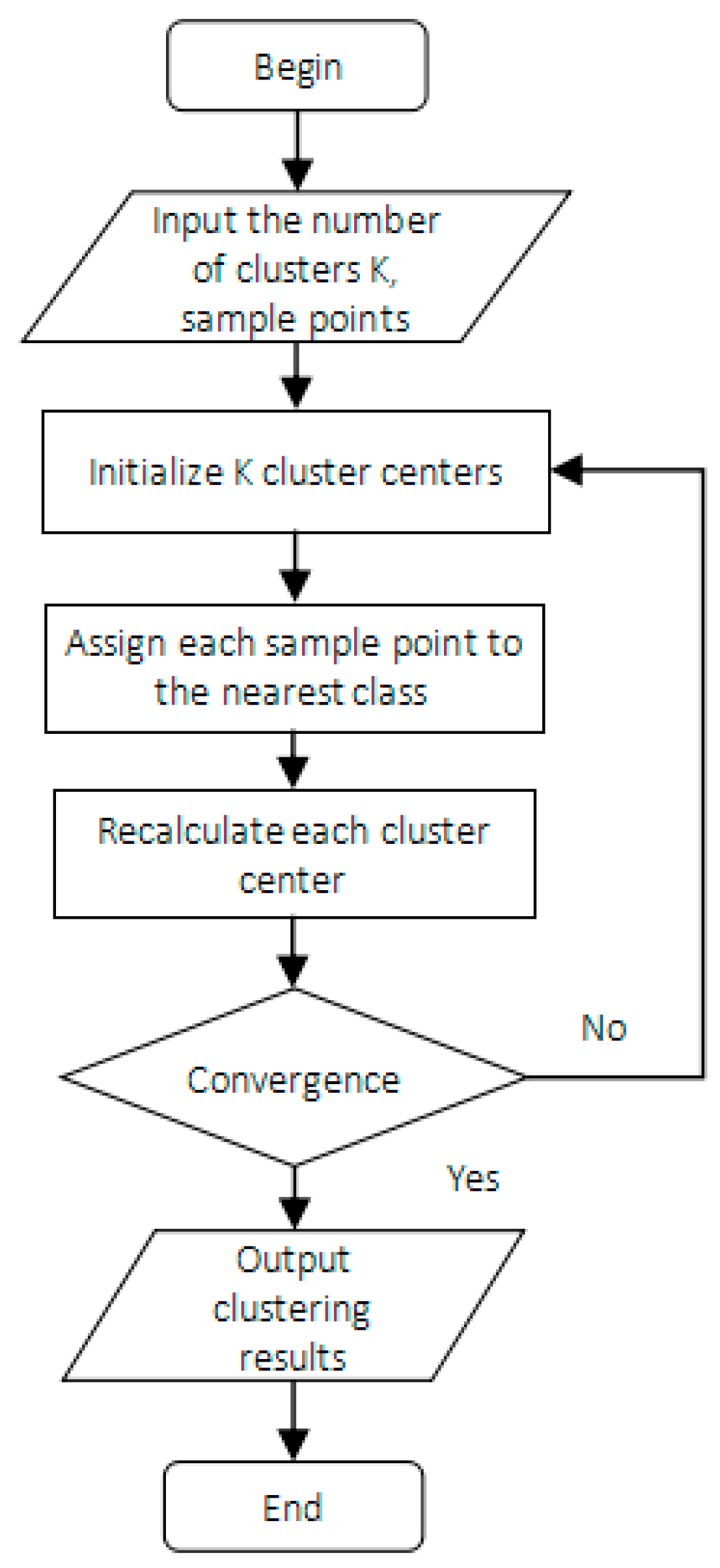
4.3. The K-Means Algorithm
A K-means algorithm is an unsupervised clustering algorithm. The basic idea of K-means is to divide the samples into k classes according to the distance between samples for a given sample set so that the distance between samples in the same class is close to each other and the distance between two different samples in different classes is as large as possible [
21,
30]. In this paper, the speed values of most mobile vehicles are relatively close, and some abnormal vehicles’ speeds are much lower or much higher than most vehicles’ speeds. Therefore, the collected average speed of vehicles is divided into three categories, which is in line with the actual traffic situation. The specific steps of speed classification are as follows. First, the velocity samples are arranged in ascending order. The lowest speed value, the fastest speed value and the medium speed value are chosen as the initial centroids of the three classes in the first round, respectively. According to the relative distance between each sample and the three centroids, all samples are grouped into three categories. In the second round, the new central point is calculated and is then selected as the new barycenter in each category. The above classification method is repeated until the classification is relatively stable.
Figure 7 shows the process of the K-means algorithm for sample classification.
4.4. The Process of the U-Test for Rogue Node Detection
Hypothesis testing is used to test specific predictions by calculating how likely it is that a pattern or relationship between variables could have arisen by chance. The basic idea of hypothesis testing is the small probability reduction method. The small probability idea believes that small probability events are basically impossible to occur in an experiment [
31,
32]. Based on this idea, we first make a hypothesis, which is very likely to be true. If, in an experiment, the experimental results deviate from the original hypothesis, then the small probability event occurs. Following this, we doubt the authenticity of the original hypothesis and reject it. The U-test is a commonly-used hypothesis testing method. The U-test uses the theory of standard normal distribution to determine the difference so as to compare whether the difference between two samples is significantly different or not [
33]. The specific steps for using the U-test for fog nodes to detect rogue nodes are as follows.
Step 1: For samples and , put forward a hypothesis H0. H0 believes there is no significant difference between the two samples, which is . At the same time, an alternative hypothesis H1 is provided, which is .
Step 2: Denote the value of the statistic
u as:
where
represents the mean value of the speed received by the fog node,
represents the overall average speed calculated by the cluster head (the same as
in this paper),
represents the standard deviation of the overall speed and
represents the number of samples received by the fog node.
Step 3: Suppose , which means the probability that the test statistic u falls in the receptive field is . This paper uses a two-sided test, and the upper and lower limits of the receptive field are ua/2 and -ua/2, respectively, that is, if the value is greater than ua/2 or less than −ua/2, the sample is different from the population, and it is initially determined to be an abnormal sample. According to the U-test, when u < 1.96, that is, the p value is greater than 0.05, it means the difference between the samples is significant. Then, hypothesis H0 is accepted and hypothesis H1 is rejected
After multiple rounds of classification and inspection, all rogue nodes are obtained. The fog node sends the information of rogue nodes to the cluster head. The cluster head also sends the rogue node information to other clusters on the road.
5. Simulation Experiment
In order to verify the performance of the proposed rogue node detection mechanism described in this paper, we use Python to conduct simulation experiments and compare our scheme with the F-RouND strategy in literature [
10] and the method described in reference (RSUs) [
7]. The F-RouND strategy of literature [
10] is used to organize moving vehicles to form vehicle clusters, and literature [
7] proposed to use RSUs to monitor the speed information of moving vehicles. In this experiment, three RSU devices are set, and the communication radius of each RSU is assumed to be 500 m.
We assume that the length of each parking cluster is 1000 m. The road has two-way lanes and the width of the road is 12 m. The communication mechanism among vehicles uses a 2 MHz 802.11p channel. According to the investigation of parked vehicles on both sides of the road in the urban environment in research [
19], the number of parked vehicles on the roadside is set as 100. The number of mobile vehicles is varied from 20–200, and the speed range of mobile vehicles is 10 km/ h–100 km/h. The specific simulation parameters used in the experiment are shown in
Table 2.
In order to compare the performance of the three schemes, this paper uses two evaluation indicators as True Positive Rate (TPR) and False Positive Rate (FPR), which are defined as follows:
TPR refers to the ratio of the number of rogue nodes correctly detected to the whole number of rogue nodes, while FPR refers to the ratio of the number of incorrectly detected rogue nodes to the number of normal nodes.
The U-test uses the theory of normal distribution to determine the difference between two samples. To verify whether the U-test is fit to detect rogue vehicles, the speed distributions of mobile vehicles are analyzed.
Figure 8 shows the histogram of the speed distribution of a randomly selected mobile vehicle within the simulation time from 100 s to 200 s in our simulation. It can be seen from
Figure 7 that the speed of the moving vehicle basically obeys the normal distribution, which meets the prerequisite of using the U-test. Therefore, the U-test is suitable for rogue node detection.
Figure 9 and
Figure 10 show that, when the proportion of rogue nodes is 20% and the number of mobile vehicles is less than 60, the scheme of this paper has significantly stronger stability than the other two schemes. The TPR value is 100% and the FPR remains at 0% when varying the number of moving vehicles, which indicates that the detection accuracy of the scheme proposed in this paper is very high. With the increase of the number of mobile vehicles, the accuracy of each scheme declines, but the decline of our proposed schemes is the smallest among the three schemes. When the number of mobile vehicles is 200, the TPR of our scheme is still more than 80%, and the FPR of our scheme is below 5%. Compared with the other two research works, our scheme achieves high performance in rogue node discovery.
It can be seen from
Figure 11 and
Figure 12 that, when the proportion of rogue nodes is increased to 30%, the proposed scheme still achieves much higher detection accuracy than the other two schemes ever though the number of automobiles is small on the road. When the number of mobile vehicles increases, the decrease of the TPR of our scheme is smaller than that of the other two comparison schemes. The FPR value can also achieve about 5%, which shows that our scheme is more accurate in abnormal node detection. Meanwhile, it can be seen from
Figure 13 that, with the increase of the ratio of rogue nodes, the proposed scheme can always achieve a relatively high TPR value. The main reason is that we use as many fog nodes as possible to discover rogue nodes, especially when the traffic is heavy. In addition, the fog network in this paper is very stable, which can face complex urban traffic conditions. In all, the algorithm proposed in this paper has higher accuracy than the other two schemes, which can identify more rogue nodes and achieve high detection accuracy.
In order to further verify the stability of the proposed algorithm, we assume that the number of moving vehicles is 200, and we compare the performance of the three schemes when changing the speed of moving vehicles. In the following experiment, assuming that the number of RSU devices is three and the proportion of rogue nodes is 20%, we explore the changes of the TPR values of the three algorithms when the standard deviation of moving vehicles’ speeds is within the range of 0.2–2.
As it can be seen from
Figure 13, when the speed standard deviation of a moving vehicle is small, the TPR values of the three algorithms are high. However, as the standard deviation is greater than 1, it can be clearly seen that the algorithm in this paper has better stability than the other two algorithms. In particular, for the F-RouND strategy in literature [
10], when the speed standard deviation of a moving vehicle is greater than 1, the TPR value decreases significantly. The reason, mainly, is this research depends too much on the physical distance of mobile vehicles on the road. When the average physical distance of the moving vehicle is long, the stability of the algorithm cannot be guaranteed. In contrast, the scheme proposed in this paper has a higher TPR value when varying the speed standard deviation and it is more stable than the other two schemes.
Next, we assume that the vehicles’ speeds follow the standard normal distribution and the standard deviation is 1. Further, the number of RSU devices is within the range of 1–5. The TPR value changes of the three algorithms are explored and shown in
Figure 14.
Moreover, assuming that the number of RSU devices is 3, the vehicles’ speed values follow the standard normal distribution, and the standard deviation is 1, the TPR values of the 3 algorithms vs. the proportion of rogue nodes is shown in
Figure 15.
As shown in
Figure 14 and
Figure 15, the algorithm proposed in this paper always has higher accuracy than the other two detection algorithms. In
Figure 14, we know that, when the number of RSUs is small, the RSU-based scheme achieves the lowest TPR among these schemes. It can be seen from
Figure 15 that, with the increase of the ratio of rogue nodes, the proposed scheme can always achieve a relatively high TPR value. It can identify more rogue nodes and can also identify normal nodes more accurately. The reason is our scheme relies on stable parked vehicles to detect rogue nodes, and the protocol performance is little affected by traffic environment changes.
In
Figure 16, the running times of the three schemes are compared. When the number of mobile vehicles is less than 75, the running times of the 3 schemes have little difference, which is less than 2000 ms. However, when the number of mobile vehicles is more than 75, the running time of the F-RouND scheme is one third slower than that of the proposed scheme. The reason is mainly because it dynamically forms the fog network using the moving vehicles on the road, which consumes a lot of time. However, the fog network formed by roadside parked cars in our scheme is much more stable. The scheme based on RSUs has the longest running time because of its complex algorithm. Theoretically, since neither the algorithm in this paper nor the F-RouND algorithm in [
10] has nested loops, the time complexity of these two algorithms is O(n). In contrast, the RSU-based strategy algorithm in literature [
7] has three layers of loops, with a high time complexity of O(n
3). In general, the algorithm in this paper has a simple structure and has a good exploration of the computing power of each vehicle and RSU equipment. It can complete the detection of rogue nodes in a relatively short time.


