A Mixed Integer Linear Programming Model with Heuristic Improvements for Single-Track Railway Rescheduling Problem

Abstract

A rescheduling algorithm for trains on a single-track railway was developed in case of disturbances that would cause conflicts between trains. This algorithm is based on mixed integer linear programming (MILP) with speed-up routines. The model considers station capacities explicitly (i.e., the number of available tracks for meeting and overtaking operations). Because the model is too hard for the solvers (CPLEX in this study) to tackle, three speed-up routines were devised when rescheduling trains. These routines are a greedy heuristic to reduce the solution space, using the lazy constraint attribute of the solver and a multiobjective approach to find a good initial feasible solution that conforms to actual railway operation. The algorithm was tested on a hypothetical rail line for different sizes of timetable instances with disturbed trains in a maximum two-hour time horizon. It managed to solve the hardest instances within a three-minute time limit thus minimizing the total weighted delay of rescheduled trains. The optimality gap metric is used to show the effectiveness and efficiencies of the speed-up heuristics developed.

1. Introduction

Among the realities of 21st-century transport are continuously increasing environmental and sustainability concerns. Rail transport, being among the most sustainable and environmentally friendly modes of transport, has been gaining importance every day. A modal shift from road and air to rail in both passenger and freight transport would be an efficient step towards sustainability. However, this shift is not very easy to achieve. Users prioritize their own satisfaction with the provided level of service over sustainability. Thus, such a modal shift can be achieved only if a satisfactory level of service is provided to users. Service quality parameters, from the user perspective for rail transport, include speed, ticket (or transport) price, reliability, punctuality and frequency. A perceivable increase in these parameters’ values would certainly encourage more passengers, freight forwarders and logistics companies to choose rail transport. These facts have pushed researchers towards seeking efficient ways to improve these level-of-service parameters. Unquestionably, the most effective method of improvement is to make new rail infrastructure investments to increase capacity, remove bottlenecks and reduce the number of potential intertrain conflicts. However, more often than not, this would be impossible due to a number of factors, such as lack of sufficient finance, land unavailability, opposition from environmentalist groups, etc. When infrastructure investment is not an option, the only remaining way is to better utilize the existing infrastructure through better operational practices. Railway operation is a very wide concept with many components, and train scheduling is one of the crucial components. Train scheduling is a rather generic term, as it includes preparation of the running timetables of the trains and real-time rescheduling for the trains in case of disturbances to train traffic. At this point, it would be useful to define the concept of rescheduling in more detail. Railways may or may not be operated with a timetable. If there exists a timetable and, in daily operation, all trains move according to the timetable, then no problems in the operation will arise. However, some trains may get delayed. Depending on the delay value, the timetable may become invalid. Delayed trains create new intertrain conflicts and, in turn, cause additional delays to be spread to other trains, and the delayed trains’ delays may increase due to such new conflicts. These newly formed delays are called “secondary delays” or “knock-on delays”. Thus, in case of delays, even if there is a timetable, it may become infeasible to follow it. In this case, a new schedule must be prepared to restore the feasibility of the train movements’ schedule. The activity of preparing a new feasible running timetable in case of real-time disruption is called rescheduling. The quality of the reschedule may be defined by its success in reducing the delays as much as possible. In practice, rescheduling is generally performed manually by human experts (called dispatchers), and the limited computational capacity of the human brain usually leads to suboptimal rescheduling decisions. The computational power of a modern computer would certainly help make better decisions. Thus, it is no surprise that computer-based decision support systems for improving rescheduling decisions has been a very popular research topic, and this study is also focused on that. The main purpose and scope of this study is rescheduling the train traffic on a single-track railway line by detecting and solving conflicts.

The most challenging fact about rescheduling is the necessity of performing the duty in a very short duration. This is because of the dynamic environment of railway operations. Trains are not static entities; they move. They can also gain new delays and make the newly constructed schedule invalid. This may necessitate more than one or even many rescheduling processes to be performed throughout the operational day. This is another indicator of the urgency of rescheduling decisions.

Train rescheduling, like almost all scheduling problems, is an NP-complete problem [1]. Even the most powerful computers of today cannot solve these kinds of problems using a brute-force approach or a pure mathematical programming approach within a reasonable duration. Some cleverer algorithms are always required. This is where the contribution of this study lies. We developed a mixed integer linear programming model to formulate the process of preparing a conflict-free schedule. Our model also explicitly considers the number of secondary lines in each station. The set of station capacity constraints used in the mathematical model, which are defined using special binary variables, is unique to this study. The tendency of studies in the literature is to relax or neglect the station capacity constraints because they increase the model size dramatically. In our model, they are explicitly considered. Such a mathematical programming approach is extremely hard to tackle for even the most powerful computers and today’s most state-of-the-art solvers. We, therefore, developed three routines for speeding the solution up: a solution space reduction algorithm based on a greedy heuristic, usage of the lazy constraint attribute of the solver and utilization of a multiobjective approach to find a good initial feasible solution. To the best of our knowledge, this is a unique combination of the specially developed routines to solve the hard train rescheduling mathematical model.

The remaining parts of the paper are structured as follows. Related work is presented next, followed by the detailed description of the mathematical model. We then introduce the speed-up routines to be able to solve the model within specified time limits. The description of the problem instances and the numerical test are given next with their results. The paper is concluded with the discussion and conclusion section.

2. Related Works

A very large number of studies about train scheduling and rescheduling have been published for decades. This may be attributed to continuously increasing railway traffic volumes and failure to improve their infrastructures through investment to cope with this situation. When it is not possible to have higher-capacity infrastructure, the natural response is to seek ways to utilize the existing infrastructure more efficiently. Generating more efficient timetables (called timetabling or scheduling) and improving dispatching decisions in case of disturbances (called rescheduling) is an applicable strategy to achieve this, hence the wide interest towards these topics [1].

In the literature, there are a variety of topics considered under the generic concept of train scheduling. These include timetable optimization, energy-efficient timetable generation, rolling stock planning, crew planning, etc. This study is focused on rescheduling; hence, we limited the literature review with studies on or closely related to train rescheduling. In addition, because this study is intended for conventional single-track intercity railway lines, studies related to high-speed lines and urban transit lines are not included in the review.

Train rescheduling is an NP-complete (nondeterministic polynomial-time complete) problem [1]. In this kind of problem, the major concern is computational workload because it exhibits a huge boost as the problem size (i.e., number of trains, number of stations, number of tracks, etc.) enlarges. Computational workload becomes even more crucial when the problem has to be solved in a very short period of time. This is the principal focus of this paper, which can be considered “a still open problem” in the literature because the approaches to the solution based on mathematical programming still need improvements in terms of computational efficiency.

For train rescheduling, as any other NP-complete problem, it is no surprise that researchers attack the problem with three main solution types: exact solutions (mostly optimizing over some criteria with a mixed integer linear programming model), metaheuristic solutions (like genetic algorithms, tabu search, simulated annealing, etc.) and other heuristics (either tailor-made or problem-specific heuristics or standard heuristics such as relaxations or branch-and-bound techniques) and simulation-based solutions. There are also a number of hybrid solution approaches, which make use of a combination of two or three of the above solution types. This will form the basis for classification in the literature review part. We will focus on the studies about rescheduling trains over the main lines.

Exact Methods: Andersson et al. [2] developed a mixed integer linear programming (MILP) model to improve the robustness of a timetable to reduce delay propagation in case of disturbances. They optimized the buffer times. Veelenturf et al. [3] developed a MILP model for rescheduling in case of disruptions with some additional binary variables that introduce the options of cancelling or rerouting some of the trains. They concluded that these options are required for switching between the original timetable and the newly constructed schedule. Sels et al. [4] aimed to minimize the expected total travel time of passengers (rather than trains) in practice with a MILP model. Their MILP also includes a lot of constraints and valid inequalities to speed up the solution process. Taslimi et al. [5] focused on the train scheduling problem to estimate the arrival (or travel) times of freight trains. Their proposed model is basically a MILP model for the train rescheduling problem. Similar to our study, this study also makes use of the lazy constraint attribute to speed up the run.

Metaheuristics: Samà et al. [6] solved the train rescheduling and rerouting problem. They developed an ant colony optimization model for this purpose. Šemrov et al. [6] utilized a reinforced learning approach, Q-learning, for rescheduling a single-track line in case of large disruptions. They used several datasets to train the agent and then finally tested it with a real single-track line in Slovenia.

Other or problem-specific heuristics: Liu and Dessouky [7] studied a complex railway line that serves both passenger and freight traffic. They combined group-based decomposition (decomposing the traffic into passenger trains and freight trains) and train-based decomposition (treating each freight train separately to generate the feasible schedule). Ait-Ali et al. [8] studied the Lagrangian dual problem of the train timetabling problem. They claimed that this kind of dual problem traditionally had been solved using an aggregate approach in which all train requests had been involved in the dual problem. However, in this study, the dual information from all requested train paths were treated individually, which was called by the authors “disaggregate bundling”. Josyula et al. [9] explored the potential of parallel programming applications to train scheduling and succeeded in applying it. They developed tree-based depth-first search heuristics to be implemented in parallel in a multicore computer. Gao and Niu [10] worked on the scheduling problem for a mixed-traffic high-speed rail line where overtaking is allowed. They sought ways to extend the typically short time windows found in the train scheduling literature. In order to overcome the computational complexity generated by this problem while working on Lagrangian-based decomposition algorithms, they proposed an improved alternating direction method of multipliers. Sinha et al. [11] focused on generating feasible scheduling solutions with less computational time and workload. The authors considered a railway network without central control. They also worked on a two-level control approach in which low-level controllers prepare solutions for their area of responsibility and their high-level supervisors evaluate the solutions. Authors proposed greedy heuristics to improve this implementation. Bettinelli et al. [12] developed greedy heuristics to solve the conflicts that arise from a distorted timetable. They scheduled the trains one at a time, thus resolving the conflicts arising on the run. Their algorithm is also suitable for parallel computing. Şahin [13] developed two heuristic methods for the single-line rescheduling problem. One was a greedy heuristic method imitating the decision behavior of train dispatchers in the Turkish State Railways network. The other one was a heuristic with a look-ahead component to give improved results. Filcek et al. [14] studied the rescheduling problem in case of closed tracks for maintenance tasks. They developed a hierarchical heuristic algorithm that treats line closures and train runs together and reconstructs a feasible schedule within a short duration. Tiong et al. [15] studied improving dispatching decisions related to overtakes in double-track sections. They demonstrated the use of an “odds ratio” as an aiding tool to dispatchers.

Hybrid Methods: Martin-Iradi and Hopke [16] considered the periodic and symmetric train timetabling problems and utilized a time–space graph formulation to solve them. They aimed to minimize the total travel times of passengers rather than trains. They named their solution method the “dive-and-cut-and-price” method, and it made use of different heuristics, such as neighborhood search, Bender’s cuts and column generation. Högdahl et al. [17] used a multiobjective approach because timetable robustness and minimization of the planned running times in the timetable are indeed contradictory objectives. They proposed a timetable model for a single unidirectional track and applied some enhancement procedures based on a microscopic simulation fed and calibrated with random delay data. Sparing and Goverde [18] considered a periodic timetable for a network with unidirectional lines. Their MILP model determines the order of the trains so that the minimum possible cycle period is minimized, and it then generates a feasible timetable for that order. They employed several heuristics to reduce the search space so solvers can tackle the resulting large-scale MILP. Cavone et al. [19] employed a three-step solution algorithm for train rescheduling. Once a disturbance occurs and the original timetable becomes infeasible, they construct and solve a MILP for a predetermined and relatively short time horizon. Second, they apply a problem-specific heuristic to incorporate the trains included in the first timetable into the timetable of currently unaffected trains. Third, they apply an offline cross-efficiency fuzzy data envelopment analysis to the resulting timetables and real-time operations. Li and Ni [20] solved the train timetabling problem with a multi-agent simulation for constraint satisfaction. They stated that the train timetabling problem creates a large combinatorial space, and thus, they utilized an agent actor–critic algorithm to decompose this space into multiple spaces that are independent from each other. This algorithm is neural network-based. Samà et al. [21] proposed a MILP model based on the alternative graph formulation that this team generally uses. After a problem instance was solved, they classified the efficiency of the optimum solution generated with data envelopment analysis. This was made to improve the formulation rather than the solution itself. Altazin et al. [22] used two approaches at the same time: multiobjective optimization and macroscopic simulation. The optimization model was used to make decisions including adding stops, canceling stops, terminating trains early and canceling trains. Macroscopic simulation was then used to evaluate the performance of these decisions. Törnquist and Persson [23], Acuna-Agost et al. [24] and Törnquist Krasemann [25] used the same MILP formulation as the basis for their solutions, which were developed for a line with flexible number of parallel tracks, each being able to handle trains in both directions. These models, coupled with a number of other properties, generate too many binary variables to tackle within a reasonable duration. Thus, all teams employed different heuristics of their own. The first team [23] classified the conflict resolution measures into change of track, order swap and both. They then set a heuristically determined upper bound on the number of measures with respect to the original timetable and pathing. Acuna-Agost et al. [24] used three approaches to obtain suboptimal but good-enough solutions: right-shift rescheduling, a MILP-based local search method and an iterative MILP-based local search method. Note that all approaches require an initial timetable with all choices of lines and platforms, and thus they are not applicable to single-track railways where there is no timetable, such as in the US freight railways case. Törnquist Krasemann [25] utilized a greedy algorithm to solve the problem.

We believe that MILP methods should gain more attention in solving the rescheduling problem. Their state-of-the-art commercial software are getting more powerful. They can also cooperate with tailor-made heuristics, simulation-based approaches and other innovative methods like constraint programming. Therefore, they exhibit quite-high potential for the future.

3. Model and Methods

3.1. The Mathematical Model

We developed a MILP (Mixed Integer Linear Programming) model, which is adapted from [1]; most of the model components are explained in much greater detail there for the interested reader. In this section, we explain the essential features of the mathematical model. The model has some resemblance to job–shop scheduling, and it contains the standard constraints required for scheduling trains over a single-track railway line. These standard constraints include the minimum possible departure times, minimum running times between adjacent stations, minimum dwell times and/or train continuities within the stations and minimum headways between trains in the same direction and between trains in the opposite direction. In addition to those standard constraints and constraints that define meetings, followings and overtakes, there are some other constraints to consider regarding station and siding capacities (i.e., number of parallel tracks within stations and sidings available for meeting and overtaking operations) for realistic modeling. If a station or siding has n parallel tracks and at least n + 1 trains try to occupy the tracks in overlapping time periods, then the station’s capacity will be exceeded. Thus, to get a comprehensive model of station capacities, we enumerated all cases where the numbers of eastbound and westbound trains add up to n + 1. In this study, we focused on stations having one secondary track and two secondary tracks, which covers most practical situations. Traditionally, the meeting of two particular trains in a particular station is defined by one binary variable. If this station has only one secondary line, then this is also sufficient for modeling the station capacity. However, in our model, to correctly model the station capacities of stations having two secondary lines, meetings were defined with two binary variables per train couple. This will be explained shortly.

For modeling followings and overtakes, a special definition is not needed at all. The definitions in the model proposed by Jovanovic in his dissertation in 1989 will suffice [1].

Formal Mathematical Model for Scheduling Train Movements on a Single-Track Railway Line

Before presenting the model, it is necessary to state some definitions and assumptions. The model was developed for a hypothetical line, and all trains were assumed to traverse the entire line. Two opposite directions were nominated as “eastbound” and “westbound”. In the indexing scheme, stations were numbered from 1 to the total number of stations, and the station numbers increased in the eastbound direction. The number of tracks in the eastbound and westbound termini were assumed to be infinite. In the notations, if a symbol denotes a vector, then it is written in bold. The model was coded in AIMMS software using the latest version of CPLEX as the solver. The sets, indices, parameters, continuous decision variables and binary decision variables used in the model are defined in Table 1, Table 2, Table 3, Table 4 and Table 5, respectively.

Table 1. Sets.

Symbol	Definition
S	Set of stations
S1	Set of stations with one secondary track.
S2	Set of stations with two secondary tracks.
E	Set of eastbound trains
W	Set of eastbound trains

Table 2. Indices and other symbols.

Symbol	Definition
e, f, g, h	Eastbound train indices
w, x, v, z	Westbound train indices
s, t	Station indices
sF	The first station (western terminus) of the modeled railway line.
sL	The last station (eastern terminus) of the modeled railway line.

Table 3. Parameters and objective function.

Symbol	Definition
${\delta }_e$	Entrance time of eastbound train e into the system. Train e cannot depart the western terminus before this time.
${\widehat{\delta }}_w^{}:$	Entrance time of westbound train w into the system. Train w cannot depart the eastern terminus before this time.
Te	Vector of minimum travel times of eastbound train e between adjacent stations.
Tw	Vector of minimum travel times of westbound train w between adjacent stations.
${\sigma }_e^s$	Minimum dwell time of eastbound train e at station s as required by timetable (equal to 0 if train e has no scheduled stop at station s or there is no timetable at all). ∀ e ∈ E, ∀ s ∈ S\{sF, sL}
${\widehat{\sigma }}_w^s$	Minimum dwell time of westbound train w at station s as required by timetable (equal to 0 if train w has no scheduled stop at station s or there is no timetable at all). ∀ w ∈ W, ∀ s ∈ S\{sF, sL}
${\eta }_{e,f}^s$	Minimum arrive–arrive headway between eastbound train e and eastbound train f at station s. ∀ e, f ∈ E, e ≠ f, ∀ s ∈ S\{sF}
${\widehat{\eta }}_{w,x}^s$	Minimum arrive–arrive headway between westbound train w and westbound train x at station s. ∀ w, x ∈ W, w ≠ x, ∀ s ∈ S\{sL}
${\beta }_{e,f}^s$	Minimum depart–depart headway between eastbound train e and eastbound train f at station s. ∀ e, f ∈ E, e < f, ∀ s ∈ S\{sL}
${\widehat{\beta }}_{w,x}^s$	Minimum depart–depart headway between westbound train w and westbound train x at station s. ∀ w, x ∈ W, w < x,∀ s ∈ S\{sF}
${\rho }_{e,w}^s$	Minimum arrive–depart headway when eastbound train e is to depart from station s after arrival of westbound train w. ∀ e ∈ E, w ∈ W, ∀ s ∈ S\{sL}
${\widehat{\rho }}_{e,w}^s$	Minimum arrive–depart headway if westbound train w is to depart from station s after arrival of eastbound train e. ∀ e ∈ E, w ∈ W, ∀ s ∈ S\{sF}
M	A large enough positive integer.
${\alpha }_e^{}$	Scheduled arrival time of eastbound train e at station sL in the timetable. In case of nontimetabled operation, minimum possible arrival time may be used.
${\widehat{\alpha }}_w^{}$	Scheduled arrival time of westbound train w at station sF in the timetable. In case of nontimetabled operation, minimum possible arrival time may be used.
F	Total weighted delay (tardiness) function.

Table 4. Continuous decision variables.

Symbol	Definition
$a_e^s$	Arrival time of eastbound train e at station s. Not defined for s = sF, where train e enters the system. Arrival time of train e at sF is a parameter, not a decision variable.
$d_e^s$	Departure time of eastbound train e from station s. Not defined for station s = sL
${\widehat{a}}_w^s$	Arrival time of westbound train w at station s. Not defined for station s = sL, where train w enters the system. Arrival time of train w at station sL is a parameter, not a decision variable.
${\widehat{d}}_w^s$	Departure time of westbound train w from station s. Not defined for station sF
${\tau }_e^{}$	Delay (tardiness) of eastbound train e in the eastern terminus.
${\widehat{\tau }}_w^{}$	Delay (tardiness) of westbound train w in the western terminus.

Table 5. Binary decision variables.

Symbol	Definition
$b_{e,f}^s$	1, if eastbound train e departs from station s before eastbound train f and 0 otherwise. Defined for s ≠ sL and e < f.
${\widehat{b}}_{w,x}^s$	1, if westbound train w departs from station s before westbound train x and 0 otherwise. Defined for s ≠ sF and w < x.
$\overline{c_{e,w}^s}$	1, if eastbound train e and westbound train w meet at station s (s ∈ S1) and 0 otherwise.
$c_s^{e,w}$	1, if eastbound train e and westbound train w meet at station s (s ∈ S2 + {sF}) AND train e enters the station before train w and 0 otherwise.
${\widehat{c}}_s^{e,w}$	1, if eastbound train e and westbound train w meet at station s (s ∈ S2 + {sL}) AND train w enters the station before train e and 0 otherwise.

Safety is paramount in rail operations. In practice, safety against intertrain collisions is provided by the signaling system. The signaling system ensures sufficient separation between trains so that they do not undergo any risk of collision. Constraints and headway concepts in the mathematical model are defined in such a way that any unsafe movement which would be prevented by the signaling system will lead to an infeasible solution by violation of the related constraints.

The model itself is given below.

Objective Function:

$$\mathrm{Min}{\displaystyle \sum _{e\in E}F({\tau }_e)+}{\displaystyle \sum _{w\in W}F({\widehat{\tau }}_w)}$$

(1)

The Objective Function (1) is a linear combination of delays of each (eastbound and westbound) train. This is a fairly standard objective function found in most studies in the literature. The verbal expression of it is “Minimization of the Total Weighted Delay”. This kind of objective function was selected because it reflects the overall punctuality of the rescheduling process. The delay of each train causes the objective value to increase. A weighted delay provides a more realistic model of railway operations than an unweighted total delay or a simple sum of delays. From the train operating company’s point of view, not every train is of equal importance. Some trains are more important than others and are thus assigned a higher priority by the company. This is reflected in the weights. The higher the train’s priority is, the higher the weight of that train (and contribution of a delay unit of that train to the objective value) is. Note that the weighted delays of the trains are being summed up, not the passengers or the payloads. It is possible to sum up the delays of passengers rather than trains, but this would be appropriate for studies mostly on urban rail lines rather than an intercity line, which is our focus here. Intercity railway lines are typically used by both passenger and freight trains. Future work may include a change in objective function, such as minimizing total weighted knock-on delay time.

Minimum Departure and Arrival Time Constraints:

$$d_e^{s_F}\ge {\delta }_e\forall e\in E$$

(2)

$${\widehat{d}}_w^{s_L}\ge {\widehat{\delta }}_w\forall w\in W$$

(3)

Constraints (2) and (3) prevent any train from departing from the related terminus before it actually enters the system.

Delay Definition Constraints:

$${\tau }_e^{}\ge a_e^{s_L}-{\alpha }_e,\forall e\in E$$

(4)

$${\widehat{\tau }}_w^{}\ge {\widehat{a}}_w^{s_F}-{\widehat{\alpha }}_w,\forall w\in W$$

(5)

Because the variables found in the respective left-hand sides of Constraints (4) and (5) define the delay and are nonnegative, if any train arrives earlier than its scheduled arrival time, then delay takes the value zero. By this definition, early arrivals are allowed, but they do not improve the objective value.

Minimum Running Time Constraints:

$$a_e^{s+1}\ge d_e^s+T_e^s\forall e\in E,s\in S\backslash s_L$$

(6)

$${\widehat{a}}_w^s\ge {\widehat{d}}_w^{s+1}+{\widehat{T}}_w^s\forall w\in W,s\in S\backslash s_L$$

(7)

Constraints (6) and (7) enforce the minimum running times between the adjacent stations.

Minimum Dwell Time Constraints:

$$d_e^s\ge a_e^s+{\sigma }_e^s\forall e\in E,s\in S\backslash \{s_F,s_L\}$$

(8)

$${\widehat{d}}_w^s\ge {\widehat{a}}_w^s+{\widehat{\sigma }}_w^s\forall w\in W,s\in S\backslash \{s_F,s_L\}$$

(9)

Constraints (8) and (9) enforce the minimum dwell times of the trains as required by the timetable. In case of either a nontimetabled operation or no scheduled stops at station s, these enforce the train continuities.

Following and Overtaking Constraints for Eastbound Trains:

$$d_e^s\ge d_f^s+{\beta }_{e,f}^s-M\ast b_{e,f}^s\forall e,f\in E,e<f,s\in S\backslash s_L$$

(10)

$$d_f^s\ge d_e^s+{\beta }_{f,e}^s-M\ast (1-b_{e,f}^s)\forall e,f\in E,e<f,s\in S\backslash s_L$$

(11)

$$a_e^{s+1}\ge a_f^{s+1}+{\eta }_{e,f}^{s+1}-M\ast b_{e,f}^s\forall e,f\in E,e<f,s\in S\backslash s_L$$

(12)

$$a_f^{s+1}\ge a_e^{s+1}+{\eta }_{f,e}^{s+1}-M\ast (1-b_{e,f}^s)\forall e,f\in E,e<f,s\in S\backslash s_L$$

(13)

Constraints (10) and (12) are active if eastbound train f departs station s before eastbound train e. Constraint (10) ensures that there is sufficient headway between the two trains in departure. Constraint (12) ensures that train e does not overtake train f in the mainline track section and also that there is sufficient headway between them upon arrival at the next station. Constraints (11) and (13) are active if eastbound train e departs station s + 1 before eastbound train f. Constraint (11) ensures that there is sufficient headway between the two trains in departure. Constraint (13) ensures that train f does not overtake train e in the mainline track section and also there is sufficient headway between them upon arrival at the next station.

Following and Overtaking Constraints for Westbound Trains:

$${\widehat{d}}_w^s\ge {\widehat{d}}_x^s+{\widehat{\beta }}_{w,x}^s-M\ast {\widehat{b}}_{w,x}^s\forall w,x\in W,w<x,s\in S\backslash s_F$$

(14)

$${\widehat{d}}_x^s\ge {\widehat{d}}_w^s+{\widehat{\beta }}_{x,w}^s-M\ast (1-{\widehat{b}}_{w,x}^s)\forall w,x\in W,w<x,s\in S\backslash s_F$$

(15)

$${\widehat{a}}_w^s\ge {\widehat{a}}_x^s+{\widehat{\eta }}_{w,x}^s-M\ast {\widehat{b}}_{w,x}^{s+1}\forall w,x\in W,w<x,s\in S\backslash s_F$$

(16)

$${\widehat{a}}_x^s\ge {\widehat{a}}_w^s+{\widehat{\eta }}_{x,w}^s-M\ast (1-{\widehat{b}}_{w,x}^{s+1})\forall w,x\in W,w<x,s\in S\backslash s_F$$

(17)

Constraints (14)–(17) work exactly the same as Constraints (10)–(13). The only difference is in the index orders in the respective direction of travel.

Preventing a Slow Train from Overtaking a Fast Train:

$$\forall e,f\in E,s\in S\backslash s_L|e<f\&{\delta }_e\le {\delta }_f$$

(18)

$${\widehat{b}}_{w,x}^s=1\forall w,x\in W,s\in S\backslash s_F|w<x\&{\widehat{\delta }}_w\le {\widehat{\delta }}_x$$

(19)

In general practice, slow trains are not allowed to overtake faster trains. We utilized this fact to reduce the size of the solution space. In the model, it is assumed that trains are indexed according to their speeds and that these indices get larger as trains go slower. Constraints (18) and (19) tell that if a faster train enters the line before a slower train, then it will always precede the slower train.

Preventing Alternate Overtakes:

$$b_{e,f}^{s+1}\ge b_{e,f}^s\forall e,f\in E,s\in S\backslash s_L|e<f\&{\delta }_e>{\delta }_f$$

(20)

$${\widehat{b}}_{w,x}^s\ge {\widehat{b}}_{w,x}^{s+1}\forall w,x\in W,s\in S\backslash s_F|w<x\&{\widehat{\delta }}_w>{\widehat{\delta }}_x$$

(21)

This follows the same principle as preventing a slow train from overtaking a fast train (Constraints (20) and (21)): this time, if a fast train overtakes a slower train, then it will always precede the slower train afterwards.

Forcing Meeting Constraints:

$${\displaystyle \sum _{s\in s_1}\overline{c_{e,w}^s}+{\displaystyle \sum _{s\in S_2+\left\{s_F\right\}}{c}_{e,w}^s+{\displaystyle \sum _{s\in S_2+\left\{s_L\right\}}{\widehat{c}}_{e,w}^s=1}}}\forall e\in E,w\in W$$

(22)

Constraint (22) ensures that each train couple will meet once and only once.

Meeting at s_F:

$$d_e^{s_F}\ge {\widehat{a}}_w^{s_F}+{\rho }_{e,w}^{s_F}-M\ast (1-c_{e,w}^{s_F})\forall e\in E,w\in W$$

(23)

Meeting at s_L:

$${\widehat{d}}_w^{\left|S\right|}\ge a_e^{s_L}+{\widehat{\rho }}_{e,w}^{s_L}-M\ast (1-{\widehat{c}}_{e,w}^{s_L})\forall e\in E,w\in W$$

(24)

Constraints (23) and (24) are active if trains e and w meet at a terminus of the line. In that case, the waiting train at the terminus is allowed to depart the terminus only after the train it meets arrives at the terminus.

Meeting Constraints for Intermediate Stations with One Secondary Line-1:

$$d_e^s\ge {\widehat{a}}_w^s+{\rho }_{e,w}^s-M\ast (1-\overline{c_{e,w}^s})\forall e\in E,w\in W,s\in S_1$$

(25)

Constraint (25) is active if eastbound train e and westbound train w meet at intermediate station s with one secondary line. It then forces train e to depart at least the length of the arrive–depart headway later than the arrival time of train w.

Meeting constraints for intermediate stations with one secondary line-2:

$${\widehat{d}}_w^s\ge a_e^s+{\widehat{\rho }}_{e,w}^s-M\ast (1-\overline{c_{e,w}^s})\forall e\in E,w\in W,s\in S_1$$

(26)

Constraint (26) is active if eastbound train e and westbound train w meet at intermediate station s, with one secondary line. It then forces train w to depart at least the length of the arrive–depart headway later than the arrival time of train e.

$$d_e^s\ge {\widehat{a}}_w^s+{\rho }_{e,w}^s-M\ast [1-(c_{e,w}^s+{\widehat{c}}_{e,w}^s)]\forall e\in E,w\in W,s\in S_2$$

(27)

Constraint (27) is active if eastbound train e and westbound train w meet at intermediate station s with two sidings. It then forces train e to depart at least the length of the arrive–depart headway later than the arrival time of train w. Constraint (22) ensures that at most one of the binary variables can be equal to one.

$${\widehat{d}}_w^s\ge a_e^s+{\widehat{\rho }}_{e,w}^s-M\ast [1-(c_{e,w}^s+{\widehat{c}}_{e,w}^s)]\forall e\in E,w\in W,s\in S_2$$

(28)

Constraint (28) is active if eastbound train e and westbound train w meet at intermediate station s with two sidings. It then forces train w to depart at least the length of the arrive–depart headway later than the arrival time of train e. Constraint (22) ensures that at most one of the binary variables can be equal to one.

$${\widehat{a}}_w^s\ge a_e^s+1-M\ast (1-c_{e,w}^s)\forall e\in E,w\in W,s\in S_2$$

(29)

$$a_e^s\ge {\widehat{a}}_w^s-M\ast (1-{\widehat{c}}_{e,w}^s)\forall e\in E,w\in W,s\in S_2$$

(30)

Constraints (29) and (30) introduce the definition of binary meeting variables for the stations with two secondary lines. Constraint (29) is active when $c_{e,w}^s=1$, which is when eastbound train e arrives at station s before westbound train w. Constraint (30) is active when ${\widehat{c}}_{e,w}^s=1$, which is when westbound train w arrives at station s before eastbound train e. In case of simultaneous arrival, the model will treat the situation as if the westbound train arrived first. The station or siding capacity constraints will be given as follows, first for the stations with one secondary line and then for the stations with two secondary lines. These constraints are based on the enumeration of the possible situations such that the station or siding capacity is exceeded.

$${\displaystyle \sum _{f\in E|e<f}(b_{e,f}^s-}{b}_{e,f}^{s-1})\le 1\forall e\in E,s\in S_1$$

(31)

Constraint (31) dictates that no eastbound train can overtake more than one eastbound train at station s, which has one secondary line.

$${\displaystyle \sum _{w,x\in W|w<x}\left({\widehat{b}}_{w,x}^s-{\widehat{b}}_{w,x}^{s+1}\right)}\le 1\forall w\in W,s\in S_1$$

(32)

Constraint (32) is the same as Constraint (31), but for westbound trains.

$$\left(b_{e,f}^s-b_{e,f}^{s+1}\right)+\overline{c_{e,w}^s}\le 1\forall e,f\in E|e<f,w\in W,s\in S_1$$

(33)

Constraint (33) dictates that an eastbound train cannot overtake an eastbound train and meet with a westbound train at station s, which has one secondary line.

$$\left({\widehat{b}}_{w,x}^s-{\widehat{b}}_{w,x}^{s+1}\right)+\overline{c_{e,w}^s}\le 1\forall e\in E,w,x\in W|w<x,s\in S_1$$

(34)

Constraint (34) is the same as Constraint (31), but for two westbound trains and one eastbound train.

$$a_f^s\ge d_e^s+{\eta }_{e,f}^s-M\ast (1-b_{e,f}^{s-1})\forall e,f\in E|e<f,s\in S_1$$

(35)

Constraint (35) is active when eastbound train f (slower than e) enters station s (with one secondary line) after eastbound train e, and it then dictates that train f can enter the station only after train e clears the station.

$${\widehat{a}}_x^s\ge {\widehat{d}}_w^s+{\widehat{\eta }}_{e,f}^s-M\ast (1-{\widehat{b}}_{w,x}^{s+1})\forall w,x\in W|w<x,s\in S_1$$

(36)

Constraint (36) is the same as Constraint (35), but for two westbound trains.

$$a_e^s\ge d_f^s+{\eta }_{e,f}^s-M\ast (b_{e,f}^s+b_{e,f}^{s-1})\forall e,f\in E|e<f,s\in S_1$$

(37)

Constraint (37) is active if eastbound train e enters station s (with one secondary line) after (slower) eastbound train f and will not overtake eastbound train f at station s. It then dictates that eastbound train e can enter station s only after eastbound train f departs.

$${\widehat{a}}_w^s\ge {\widehat{d}}_x^s+{\widehat{\eta }}_{w,x}^s-M\ast ({\widehat{b}}_{w,x}^s+{\widehat{b}}_{w,x}^{s+1})\forall w,x\in W|w<x,s\in S_1$$

(38)

Constraint (38) is the same as Constraint (37), but for two westbound trains.

$${\displaystyle \sum _{f\in E|e<f}(b_{e,f}^s-}{b}_{e,f}^{s-1})\le 2\forall e\in E,s\in S_2$$

(39)

Capacity Constraints for Stations with Two Secondary Lines-2:

$${\displaystyle \sum _{w,x\in W|w<x}\left({\widehat{b}}_{w,x}^s-{\widehat{b}}_{w,x}^{s+1}\right)}\le 2\forall w\in W,s\in S_2$$

(40)

Constraints (39) and (40) prevent any train from overtaking more than two trains at station s, which has two secondary lines.

Capacity Constraints for Stations with Two Secondary Lines-3:

$${\widehat{c}}_{e,w}^s+{\widehat{c}}_{e,x}^s+{\widehat{c}}_{e,y}^s\le 2\forall e\in E,w,x,y\in W|w<x<y$$

(41)

Constraint (41) prevents more than two westbound trains from “giving way to” the same eastbound train at station s, which has two secondary lines.

$$c_{e,w}^s+c_{f,w}^s+c_{g,w}^s\le 2,\forall w\in W,e,f,g\in E|e<f<g$$

(42)

Constraint (42) is the same as Constraint (41), but for more than two eastbound trains and one westbound train.

$$a_g^s\ge d_e^s+{\eta }_{e,g}^s-M\ast [1-(b_{e,f}^s+b_{e,g}^s+b_{f,g}^s)/3]\forall e,f,g\in E|e<f<g$$

(43)

$$a_f^s\ge d_e^s+{\eta }_{e,f}^s-M\ast [1-(b_{e,f}^{s-1}+b_{e,g}^{s-1}-b_{f,g}^{s-1}+b_{e,f}^s+b_{e,g}^s)/4]\forall e,f,g\in E|e<f<g$$

(44)

$$a_f^s\ge d_g^s+{\eta }_{f,g}^s-M\ast [1-(b_{e,f}^{s-1}-b_{e,g}^{s-1}-b_{f,g}^{s-1}+b_{e,f}^s-b_{f,g}^s)/2]\forall e,f,g\in E|e<f<g$$

(45)

$$a_f^s\ge d_e^s+{\eta }_{e,f}^s-M\ast [1-(b_{e,f}^{s-1}-b_{e,g}^{s-1}-b_{f,g}^{s-1}+b_{e,f}^s+b_{e,g}^s)/3]\forall e,f,g\in E|e<f<g$$

(46)

$$a_g^s\ge d_e^s+{\eta }_{e,g}^s-M\ast [1-(b_{e,g}^{s-1}-b_{e,f}^{s-1}+b_{f,g}^{s-1}+b_{e,f}^s+b_{e,g}^s+b_{f,g}^s)/5]\forall e,f,g\in E|e<f<g$$

(47)

$$a_g^s\ge d_f^s+{\eta }_{f,g}^s-M\ast [1-(b_{e,g}^{s-1}-b_{e,f}^{s-1}+b_{f,g}^{s-1}-b_{e,f}^s+b_{e,g}^s+b_{f,g}^s)/4]\forall e,f,g\in E|e<f<g$$

(48)

$$a_e^s\ge d_f^s+{\eta }_{e,f}^s-M\ast [1-(b_{f,g}^{s-1}-b_{e,g}^{s-1}-b_{e,f}^{s-1}+b_{f,g}^s-b_{e,f}^s)/2]\forall e,f,g\in E|e<f<g$$

(49)

$$a_e^s\ge d_g^s+{\eta }_{e,g}^s-M\ast (b_{e,f}^{s-1}+b_{e,g}^{s-1}+b_{f,g}^{s-1}+b_{e,g}^s+b_{f,g}^s)\forall e,f,g\in E|e<f<g$$

(50)

$$a_e^s\ge d_f^s+{\eta }_{e,f}^s-M\ast [1-(b_{f,g}^s-b_{e,f}^s-b_{f,g}^{s-1}-b_{e,g}^{s-1}-b_{e,f}^{s-1})]\forall e,f,g\in E|e<f<g$$

(51)

Constraints (43)–(51) are active only when the summation within the bracket divided by the respective integer number gives either zero or one, depending on the case. Then, the constraints enforce that the last train to enter the station must enter later than the first departing train’s departure. This prevents the station’s capacity from being exceeded.

Capacity Constraints for Stations with Two Secondary Lines 14–22:

$${\widehat{a}}_y^s\ge {\widehat{d}}_w^s+{\widehat{\eta }}_{w,y}^s-M\ast [1-({\widehat{b}}_{w,x}^s+{\widehat{b}}_{w,y}^s+{\widehat{b}}_{x,y}^s)/3]\forall w,x,y\in W|w<x<y$$

(52)

$${\widehat{a}}_x^s\ge {\widehat{d}}_w^s+{\widehat{\eta }}_{w,x}^s-M\ast [1-({\widehat{b}}_{w,x}^{s+1}+{\widehat{b}}_{w,y}^{s+1}-{\widehat{b}}_{x,y}^{s-1}+{\widehat{b}}_{w,x}^s+{\widehat{b}}_{w,y}^s)/4]\forall w,x,y\in W|w<x<y$$

(53)

$${\widehat{a}}_x^s\ge {\widehat{d}}_y^s+{\widehat{\eta }}_{x,y}^s-M\ast [1-({\widehat{b}}_{w,x}^{s+1}-{\widehat{b}}_{w,y}^{s+1}-{\widehat{b}}_{x,y}^{s+1}+{\widehat{b}}_{w,x}^s-{\widehat{b}}_{x,y}^s)/2]\forall w,x,y\in W|w<x<y$$

(54)

$${\widehat{a}}_x^s\ge {\widehat{d}}_w^s+{\widehat{\eta }}_{w,x}^s-M\ast [1-({\widehat{b}}_{w,x}^{s+1}-{\widehat{b}}_{w,y}^{s+1}-{\widehat{b}}_{x,y}^{s+1}+{\widehat{b}}_{w,x}^s+{\widehat{b}}_{w,y}^s)/3]w,x,y\in W|w<x<y$$

(55)

$${\widehat{a}}_y^s\ge {\widehat{d}}_w^s+{\widehat{\eta }}_{w,y}^s-M\ast [1-({\widehat{b}}_{w,y}^{s+1}-{\widehat{b}}_{w,x}^{s+1}+{\widehat{b}}_{x,y}^{s+1}+{\widehat{b}}_{w,x}^s+{\widehat{b}}_{w,y}^s+{\widehat{b}}_{x,y}^s)/5]\forall w,x,y\in W|w<x<y$$

(56)

$${\widehat{a}}_y^s\ge {\widehat{d}}_x^s+{\widehat{\eta }}_{x,y}^s-M\ast [1-({\widehat{b}}_{w,y}^{s+1}-{\widehat{b}}_{w,x}^{s+1}+{\widehat{b}}_{x,y}^{s+1}-{\widehat{b}}_{w,x}^s+{\widehat{b}}_{w,y}^s+{\widehat{b}}_{x,y}^s)/4]\forall w,x,y\in W|w<x<y$$

(57)

$${\widehat{a}}_w^s\ge {\widehat{d}}_x^s+{\widehat{\eta }}_{w,x}^s-M\ast [1-({\widehat{b}}_{x,y}^{s+1}-{\widehat{b}}_{w,y}^{s+1}-{\widehat{b}}_{w,x}^{s+1}+{\widehat{b}}_{x,y}^s-{\widehat{b}}_{w,x}^s)/2]\forall w,x,y\in W|w<x<y$$

(58)

$${\widehat{a}}_w^s\ge {\widehat{d}}_y^s+{\widehat{\eta }}_{w,y}^s-M\ast ({\widehat{b}}_{w,x}^{s+1}+{\widehat{b}}_{w,y}^{s+1}+{\widehat{b}}_{x,y}^{s+1}+{\widehat{b}}_{w,y}^s+{\widehat{b}}_{x,y}^s)\forall w,x,y\in W|w<x<y$$

(59)

$${\widehat{a}}_w^s\ge {\widehat{d}}_x^s+{\widehat{\eta }}_{w,x}^s-M\ast [1-({\widehat{b}}_{x,y}^s-{\widehat{b}}_{w,x}^s-{\widehat{b}}_{x,y}^{s+1}-{\widehat{b}}_{w,y}^{s+1}-{\widehat{b}}_{w,x}^{s+1})]\forall w,x,y\in W|w<x<y$$

(60)

Constraints (52)–(60) are exactly the same as Constraints (43)–(51), except they apply to the symmetrical case.

$$c_{e,w}^s+c_{e,x}^s+c_{f,w}^s+c_{f,x}^s+(b_{w,x}^s-b_{w,x}^{s+1})\le 4,\forall e,f\in E,w,x\in W|e<f\&w<x$$

(61)

$${\widehat{a}}_w^s\ge {\widehat{d}}_x^s+{\widehat{\eta }}_{w,x}^s-M\ast [1-(c_{e,w}^s+c_{e,x}^s+c_{f,w}^s+c_{f,x}^s-{\widehat{b}}_{w,x}^{s+1})/4]\forall e,f\in E,w,x\in W|e<f\&w<x$$

(62)

$${\widehat{a}}_x^s\ge {\widehat{d}}_w^s+{\widehat{\eta }}_{w,x}^s-M\ast [1-(c_{e,w}^s+c_{e,x}^s+c_{f,w}^s+c_{f,x}^s+{\widehat{b}}_{w,x}^{s+1})/5]\forall e,f\in E,w,x\in W|e<f\&w<x$$

(63)

$$(c_{e,w}^s+c_{e,x}^s+c_{f,w}^s+{\widehat{c}}_{f,x}^s-{\widehat{b}}_{w,x}^{s+1})\le 4\forall e,f\in E,w,x\in W|e<f\&w<x$$

(64)

$${\widehat{a}}_w^s\ge {\widehat{d}}_x^s+{\widehat{\eta }}_{w,x}^s-M\ast [1-(c_{e,w}^s+c_{e,x}^s+c_{f,w}^s+{\widehat{c}}_{f,x}^s)/4]\forall e,f\in E,w,x\in W|e<f\&w<x$$

(65)

$${\widehat{a}}_x^s\ge {\widehat{d}}_w^s+{\widehat{\eta }}_{w,x}^s-M\ast [1-(c_{e,w}^s+c_{e,x}^s+{\widehat{c}}_{f,w}^s+c_{f,x}^s)/4]\forall e,f\in E,w,x\in W|e<f\&w<x$$

(66)

$$a_f^s\ge d_e^s+{\eta }_{e,f}^s-M\ast [1-(c_{e,w}^s+c_{e,x}^s+{\widehat{c}}_{f,w}^s+{\widehat{c}}_{f,x}^s)/4]\forall e,f\in E,w,x\in W|e<f\&w<x$$

(67)

$$c_{e,w}^s+{\widehat{c}}_{e,x}^s+c_{f,w}^s+{\widehat{c}}_{f,x}^s-{\widehat{b}}_{w,x}^{s+1}\le 4\forall e,f\in E,w,x\in W|e<f\&w<x$$

(68)

$${\widehat{a}}_w^s\ge {\widehat{d}}_x^s+{\widehat{\eta }}_{w,x}^s-M\ast [1-(c_{e,w}^s+{\widehat{c}}_{e,x}^s+c_{f,w}^s+c_{f,x}^s)/4]\forall e,f\in E,w,x\in W|e<f\&w<x$$

(69)

$$c_{e,w}^s+{\widehat{c}}_{e,x}^s+c_{f,w}^s+{\widehat{c}}_{f,x}^s-({\widehat{b}}_{w,x}^s-{\widehat{b}}_{w,x}^{s+1})\le 4\forall e,f\in E,w,x\in W|e<f\&w<x$$

(70)

$${\widehat{a}}_w^s\ge {\widehat{d}}_x^s+{\widehat{\eta }}_{w,x}^s-M\ast [1-(c_{e,w}^s+{\widehat{c}}_{e,x}^s+c_{f,w}^s+{\widehat{c}}_{f,x}^s-{\widehat{b}}_{w,x}^{s+1})/4]\forall e,f\in E,w,x\in W|e<f\&w<x$$

(71)

$$a_f^s\ge d_e^s+{\eta }_{e,f}^s-M\ast [1-(c_{e,w}^s+{\widehat{c}}_{e,x}^s+{\widehat{c}}_{f,w}^s+{\widehat{c}}_{f,x}^s)/4]\forall e,f\in E,w,x\in W|e<f\&w<x$$

(72)

$${\widehat{a}}_x^s\ge {\widehat{d}}_w^s+{\widehat{\eta }}_{w,x}^s-M\ast [1-({\widehat{c}}_{e,w}^s+c_{e,x}^s+c_{f,w}^s+c_{f,x}^s)/4]\forall e,f\in E,w,x\in W|e<f\&w<x$$

(73)

$${\widehat{a}}_x^s\ge {\widehat{d}}_w^s+{\widehat{\eta }}_{w,x}^s-M\ast [1-({\widehat{c}}_{e,w}^s+c_{e,x}^s+{\widehat{c}}_{f,w}^s+c_{f,x}^s)/4]\forall e,f\in E,w,x\in W|e<f\&w<x$$

(74)

$$a_f^s\ge d_e^s+{\eta }_{e,f}^s-M\ast [1-({\widehat{c}}_{e,w}^s+c_{e,x}^s+{\widehat{c}}_{f,w}^s+{\widehat{c}}_{f,x}^s)/4]\forall e,f\in E,w,x\in W|e<f\&w<x$$

(75)

$${\widehat{c}}_{e,w}^s+{\widehat{c}}_{e,x}^s+c_{f,w}^s+c_{f,x}^s+(b_{e,f}^s-b_{e,f}^{s-1})\le 4\forall e,f\in E,w,x\in W|e<f\&w<x$$

(76)

$$a_e^s\ge d_f^s+{\eta }_{e,f}^s-M\ast [1-({\widehat{c}}_{e,w}^s+{\widehat{c}}_{e,x}^s+{\widehat{c}}_{f,w}^s+{\widehat{c}}_{f,x}^s)/4]\forall e,f\in E,w,x\in W|e<f\&w<x$$

(77)

$${\widehat{c}}_{e,w}^s+{\widehat{c}}_{e,x}^s+c_{f,w}^s+{\widehat{c}}_{f,x}^s+(b_{e,f}^s-b_{e,f}^{s-1})\le 4\forall e,f\in E,w,x\in W|e<f\&w<x$$

(78)

$$a_e^s\ge d_f^s+{\eta }_{e,f}^s-M\ast [1-({\widehat{c}}_{e,w}^s+{\widehat{c}}_{e,x}^s+c_{f,w}^s+{\widehat{c}}_{f,x}^s)/4]\forall e,f\in E,w,x\in W|e<f\&w<x$$

(79)

$${\widehat{c}}_{e,w}^s+{\widehat{c}}_{e,x}^s+{\widehat{c}}_{f,w}^s+c_{f,x}^s+(b_{e,f}^s-b_{e,f}^{s-1})\le 4\forall e,f\in E,w,x\in W|e<f\&w<x$$

(80)

$$a_e^s\ge d_f^s+{\eta }_{e,f}^s-M\ast [1-({\widehat{c}}_{e,w}^s+{\widehat{c}}_{e,x}^s+{\widehat{c}}_{f,w}^s+c_{f,x}^s)/4]\forall e,f\in E,w,x\in W|e<f\&w<x$$

(81)

$$a_f^s\ge d_e^s+{\eta }_{e,f}^s-M\ast [1-({\widehat{c}}_{e,w}^s+{\widehat{c}}_{e,x}^s+{\widehat{c}}_{f,w}^s+{\widehat{c}}_{f,x}^s+b_{e,f}^{s-1})/5]\forall e,f\in E,w,x\in W|e<f\&w<x$$

(82)

$${\widehat{c}}_{e,w}^s+{\widehat{c}}_{e,x}^s+{\widehat{c}}_{f,w}^s+{\widehat{c}}_{f,x}^s+(b_{e,f}^s-b_{e,f}^{s-1})\le 4\forall e,f\in E,w,x\in W|e<f\&w<x$$

(83)

$$a_e^s\ge d_f^s+{\eta }_{e,f}^s-M\ast [1-({\widehat{c}}_{e,w}^s+{\widehat{c}}_{e,x}^s+{\widehat{c}}_{f,w}^s+{\widehat{c}}_{f,x}^s-b_{e,f}^{s-1})/4]e,f\in E,w,x\in W|e<f\&w<x$$

(84)

Constraints (61)–(84) generally enforce the following rule: “If two westbound trains and two eastbound trains will meet each other at station s, which has two secondary lines, then the last train to arrive at station s should postpone its arrival into station s until the departure of the first train in the same direction”. The values of binary variables determine which train is the last to enter station s and which train, in the direction of the last arriving train, leaves the station first. Constraints (31)–(84) also serve to prevent deadlocks. In Figure 1, a typical deadlock situation is shown. In this situation, Train 1 will not be allowed to overtake Train 3 because, if it did, it would not be allowed to meet with Train 2 at this station because of Constraints (34)–(35). Thus, it will have to wait until the departure of Train 3 from the station. Meeting constraints dictate that the departure of Train 3 from the station requires Train 4 to be held at the adjacent station (i.e., immediately preceding station in the itinerary of Train 4); thus, a situation like that in the Figure 1 will never arise.

Figure 1. Illustration of deadlock prevention.

3.2. Speed-Up Routines

The mathematical model represents the train movements on a single-track railway line quite accurately, but it also has some serious drawbacks. For instance, it models the meetings at stations with two secondary lines with two binary variables per train couple per station. This causes a significant increase in the number of binary variables. In addition, complete enumeration of all situations in which station or siding capacities are exceeded causes the number of constraints to boom. Even the most powerful computers of today will be helpless against the problem if the problem has no external interference. The good news is that a minority of these constraints will actually be binding in the optimal solution. In Figure 2, an example optimal solution produced with the model is depicted. In this hypothetical railway line, stations 4, 6, 8, 11 and 14 have one secondary line, whereas the others have two secondary lines. At least three and four trains are needed, respectively, to exceed the capacity of a station with one secondary line and a station with two secondary lines. In Figure 2, it can be seen that only three of the stations with one secondary line (4, 6, 8) were “under threat” of siding capacity violation, each from only one trio of trains. Similarly, only two of the stations with two secondary lines (9, 10) were “under threat” of capacity violation, each from only one quartet of trains. This clearly indicates that only a handful of these constraints were binding. The others were just there to make the model unnecessarily complicated and intractable. Indeed, there is one more fact that makes most of these constraints actually unnecessary: any trio or quartet of trains, unless they are all traveling in the same direction, cannot impose a threat of exceeding the capacity of more than one station. This is due to the nature of train traffic. Two trains moving in opposite directions cannot meet more than once.

Figure 2. Optimal schedule of an example instance.

3.2.1. Lazy Constraint Attribute

In AIMMS, the user is allowed to label constraints as “lazy”. When the solver recognizes lazy constraints, it does not directly include them in the model. Instead, it solves a “relaxed” model with these lazy constraints omitted. Each time it finds a feasible solution of this “relaxed” model, it checks the solution against the lazy constraints. If it detects violation of a lazy constraint, it then forms a new “relaxed” model by adding the violated lazy constraint and resolves the model. In the model, all of the station and siding capacity constraints except the ones involving only binary variables were defined as lazy constraints.

3.2.2. Solution Space Restriction Algorithm for Reducing the Number of Binary Variables and Constraints

As mentioned before, the model hosts a very large number of constraints. However, very few of the constraints for conflict resolution will actually be binding. Moreover, most of the binary variables defined for meetings will simply be zero. Therefore, if we can eliminate the constraints that are very unlikely to be binding and the binary variables which are very likely to be zero in the optimal solution, then a significant reduction in problem size and thus computation time may be achieved. Such progress was already made by defining the station or siding capacity constraints as “lazy constraints”. Hence, a heuristic solution space restriction algorithm has been developed to aid the solver in the solution procedure. It involves implementing a greedy heuristic that does not consider station capacity constraints to see what a solution may actually “look like”. Then, the actual solution will be restricted to being “properly similar” to the outcome of this greedy heuristic. The greedy heuristic is quite simple: starting from scratch, it finds all the conflicts and resolves them one by one. Finally, it arrives at a feasible solution. The heuristic tackles the constraints in “time order”: it finds the first conflict with respect to time, resolves it, then finds the next conflict and resolves it, repeating until there are no conflicts left. The decision logic of the heuristic is very simple and myopic, hence making it a greedy heuristic. When it detects the conflict, it first resolves the conflict by delaying one of the two conflicting trains. It then computes the total weighted unrecoverable delay of two trains in conflict after this local resolution. Then, it reverses the solution and resolves the conflict by delaying the other conflicting train. After that, it again computes the total weighted unrecoverable delay of two trains in conflict after local resolution. The alternative that gives the lower total weighted unrecoverable delay of two trains will be selected. The heuristic will then update the departure and arrival times of the delayed train and find the next conflict. The heuristic’s steps of execution are as follows:

Step 1. For all trains, compute the departure times from and arrival times at all stations as if all trains can move on a dedicated track with no conflicts.

Step 2 Find all of the (meeting, headway, overtaking, etc.) conflicts in the system. If there are no conflicts left, terminate and report the final solution (all departure and arrival times for all trains plus the locations of meetings and overtakes). If there is at least one remaining conflict, go to Step 3.

Step 3: Determine the possible occurrence times of the conflicts by calculating the intersection points of the train paths.

Step 4: Find the earliest conflict and resolve it.

Step 5: Update the departure and arrival times of the train to be delayed in the immediate conflict resolution, as done in Step 1, and go to Step 2.

This algorithm is guaranteed to give a feasible solution for the relaxed problem where all stations are assumed to have infinite capacity.

Restriction of the Solution Space for Meetings

Several trial runs were made in which it was experienced that, for the places where meetings between trains take place, the differences between the outcomes of the heuristically solved relaxed problem and the original problem solved to optimality were small, if any. This constitutes the rule of thumb for the solution space restriction, in that meetings between an eastbound and a westbound train were restricted to happen in one of the five stations only: the station in which the meeting occurs in the relaxed problem and two neighboring stations away from this meeting station in each direction. Note that meeting constraints (22)–(30) are defined in such a way that feasibility is always guaranteed. Constraint (22) forces the meeting to happen in one of the stations where meeting variables are defined. The other constraints guarantee satisfaction of the arrive–depart headway constraints in that station and also prevent meeting on the mainline track section. Thus, upon finding the restricted region for meetings, all of the remaining constraints and binary variables that allowed meetings between these two trains in other stations were kicked out of the model. The heuristic was coded in AIMMS. Afterwards, through proper index domain definitions of the variables and constraints, the model with the unnecessary constraints eliminated was automatically generated with AIMMS.

Restriction of the Solution Space for Followings and Overtakes

The case with followings and overtakes is not simple as in the meeting case. In this case, radical differences may arise between the heuristic outcome and the actual optimal solution. We cannot know where the fast train will “catch” the slow one (or if it will ever catch it) without actually getting the optimal solution because this depends on the solution itself. If the fast train is delayed in conflict resolutions before catching the slow train, then the distance between them will increase. On the other hand, if the slow train is delayed in conflict resolutions before the fast train catches up, then the distance between them will decrease. Therefore, the model cannot be easily reduced as much as it was for the meeting case. However, some improvements can still be made. Indeed, the fast train can catch up to the slow train in the earliest possible place if the fast train is never stopped in conflicts before catching up to the slow train, whereas the slow train is stopped and forced to wait in all conflicts before the fast train catches up. Such a case can be simulated by temporarily assigning a very high weight on the fast train’s delay (e.g., 5000 min/min) and very low weight on the slow train’s delay (i.e., 0.0001 min/min). Optionally, the fast train can be introduced into the line with a large amount of already experienced unrecoverable delay, whereas the slow train would have a long recovery time. In these cases, the heuristic will always give priority to the fast train and never give priority to the slow train in their respective conflicts. Thus, it will be possible to determine the earliest place that the fast train can catch and overtake the slow train. For all of the train couples moving in the same direction, for which the slow one enters the system before the fast one, such extreme values were set and the heuristic was run once. Then, it was assumed that the overtake can happen in one of the four stations upstream (in the involved trains’ direction) of the heuristic outcome or later. All binary variables for the stations upstream of this earliest possible station were fixed (not eliminated to be on the safe side for modeling station and siding capacities). If any fast train entered the line earlier than a slow train in the same direction by enough of a margin, then we assumed that the fast train would get further away and that these two trains would never interact, thus all related binary variables and constraints were then eliminated.

Use of a “Min–Max” Problem for the Initial Feasible Solution

We observed that if the objective function were formulated as the maximum (weighted) delay, the solver then found the optimal solution quicker than the formulation with total (weighted) delay as the objective function. Solvers can accept initial feasible solutions and use these solutions to expedite the solution procedure by providing good upper bounds. In all of these problems, before solving the actual problem with total weighted delay, a problem with the maximum weighted delay objective was solved as coupled with the heuristic problem reduction algorithm mentioned above. The optimal solution of this problem was then fed as the initial feasible solution. At that stage, a new constraint was added to the model that prevents the maximum delay value from being higher than the optimal value of the min-max problem. This procedure proved to be quite effective in reducing running time. It also provided the opportunity to obtain better-quality solutions (from a railway operation perspective, which prefers to distribute the delay among multiple trains over delaying a single train excessively). This is illustrated in Table 6. Among the two alternative solutions given in the table, if the objective is to minimize total delay, then the algorithm would choose Solution 2. However, from a railway operation perspective, Solution 1 is more preferable. Thus, a multiobjective optimization approach was adopted. The final objective is still to minimize total weighted delay, but the maximum weighted delay will be constrained not to be higher than the maximum weighted delay obtained in the initial feasible solution with the maximum weighted delay objective.

Table 6. An example of an unfavorable solution by total delay approach.

	Delays in Solution 1 (min)	Delays in Solution 2 (min)
Train 1	5	29
Train 2	5	0
Train 3	5	0
Train 4	5	0
Train 5	5	0
Train 6	5	0

Before presenting the numerical tests and results, as a summary, the entire algorithm works in the following execution order: gathering all parameter values, running the solution space restriction algorithm for meetings, running the solution space restriction algorithm for followings and overtakes, construction of the model, identification of lazy constraints, solving the model with the maximum weighted delay objective and solving the model with the total weighted delay objective.

4. Numerical Tests and Results

In this section, we present the numerical tests and the results of the solved instances.

4.1. Railway Line

The model was implemented on a hypothetical railway line. Its topology was based on the historical topology of the Arifiye–Çukurhisar section of Turkey’s İstanbul–Ankara conventional railway line. The entire section is single-track, and Arifiye and Çukurhisar are the western and eastern termini, respectively. In the trial runs, only the topology (names of the stations and sidings and numbers of secondary tracks in the stations and sidings) was real. The minimum running times and train types (which will be presented below) were all hypothetical. In this section, instead of station names, only station numbers, which increase in the eastbound direction, will be used. In the line, stations 5, 8, 11, 13 and 15 have one secondary line and the others, except for the two termini with assumed infinite capacities, have two secondary lines. This information is again from the historical topology of the line.

4.2. Trains

We assumed that three different types of trains operate over the line: fast, semi-fast and slow. All types of trains have their respective minimum running times defined in each mainline track segment. We assigned odd numbers to the eastbound trains and even numbers to the westbound trains. Trains were numbered with respect to speed categories; fast (and higher priority) trains were assigned the smaller numbers. Among trains of the same type, the one entering the line first got the smaller number (hence the higher priority). Because we solved a weighted delay problem, every train had to be assigned a weight. Unsurprisingly, faster trains had higher weights. Thus, their delays worsened the objective function more than the slower trains’ delays. Trains in the problem instances are summarized in Table 7.

Table 7. Trains in the problem instances.

Train Number	Direction	Train Type	Weight
1	Eastbound	Fast	6
2	Westbound	Fast	6
3	Eastbound	Fast	6
4	Westbound	Semi-fast	4
5	Eastbound	Semi-fast	4
6	Westbound	Semi-fast	4
7	Eastbound	Semi-fast	4
8	Westbound	Slow	3
9	Eastbound	Slow	3
10	Westbound	Slow	3
11	Eastbound	Slow	3

4.2.1. Orders and Frequency of Trains

The order in which trains entered the line had a great effect on the actual difficulty of the instance. When a faster (higher priority) train entered the line before a slower (lower priority) train in the same direction, no overtaking was allowed between those two trains. Thus, all binary variables related to the following and overtaking of these two trains could be either fixed or omitted from the model (see Section 3.2.2). Furthermore, because the distance between these two trains could be safely assumed to grow, virtually all headway constraints between these two trains would be guaranteed to be nonbinding. Given these facts, one can indeed easily “cheat” by selecting the problem instances properly, i.e., sending the faster trains first and then the slower trains. This was not the case for this study. In all instances, trains entered the line from the slowest to the fastest. In Table 8, the entrance time orders are given. The order is from the left to the right. Different instances are defined by the entrance times of the trains plus the entrance delays. However, the entrance time orders do not differ. All of them follow the same scheme. In the table, “s” stands for “slow”, “s-f” stands for “semi-fast” and “f” stands for “fast”.

Table 8. Train entrance time orders.

Eastbound	9 (s)	11 (s)	5 (s-f)	7 (s-f)	1 (f)	3 (f)
Westbound	8 (s)	10 (s)	4 (s-f)	6 (s-f)	2 (f)	-

Furthermore, the headways between the entrances of the trains would produce an effect. If the trains are too infrequent, most (if not all) of the following- and overtaking-related constraints would be nonbinding. Because this will make respective binary variables useless, a solution space restriction algorithm will fix or eliminate most of them. Table 9 illustrates how the entrance time order can affect problem complexity. Because the solution space restriction algorithm does not eliminate any continuous variables, no difference in the number of them would be observed. The reduction is in the number of constraints and binary variables. It can be clearly seen that, with the same number of trains, it would be possible to create instances that are much easier to solve. However, we did not adopt this approach. Instead, in these instances, trains were introduced into the system in small headways and from the slowest to the fastest. Readers can think our approach as a “worst-case scenario” approach.

Table 9. Effect of train order and number of eastbound and westbound trains on problem size.

Problem Type	# of Trains	# of Binary Variables	# of Constraints
Fastest to slowest, large intervals	3 + 3	63	662
Fastest to slowest, large intervals	6 + 5	167	3667
Slowest to fastest, small intervals	3 + 3	119	1571
Slowest to fastest, small intervals	6 + 5	462	>41,000

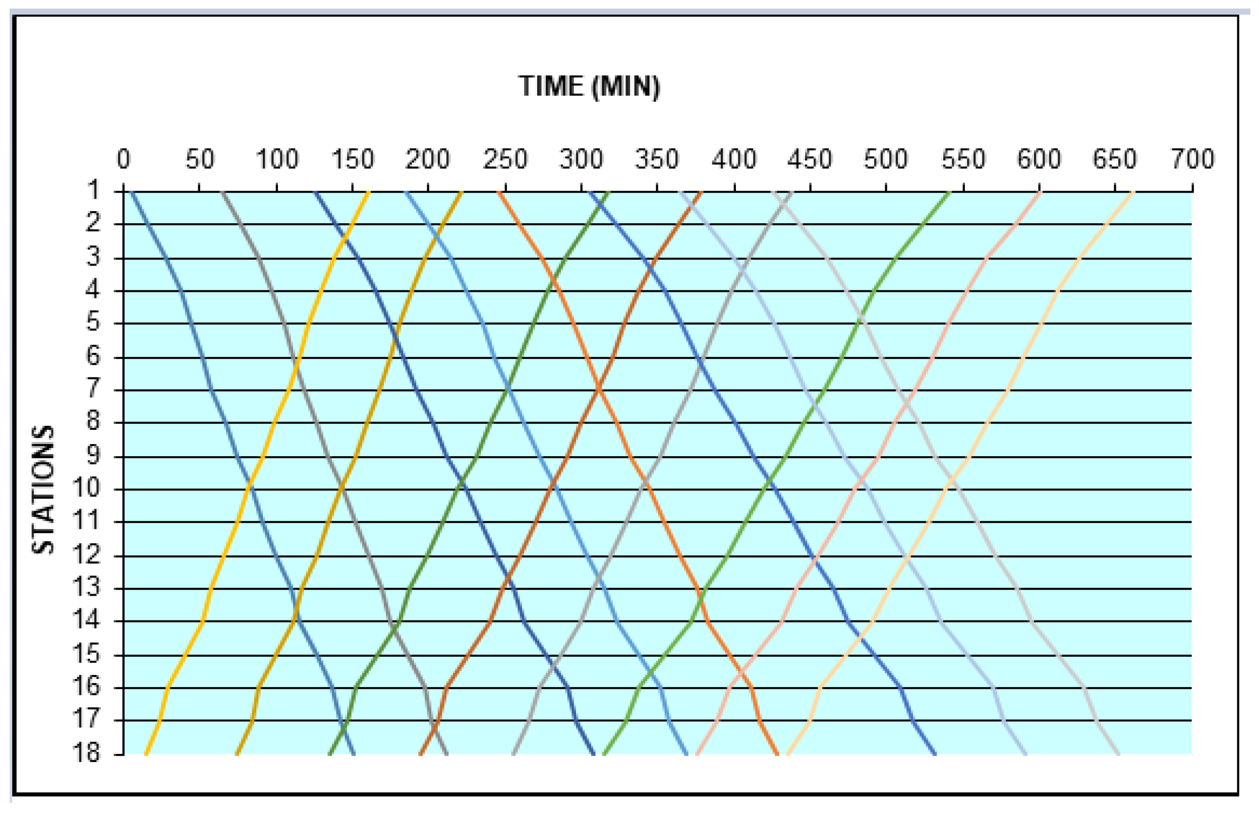
To further demonstrate the effect of train order and frequency on problem difficulty (or complexity), a special instance with eight eastbound and eight westbound trains was prepared. In this instance, trains were introduced into the system from the fastest to the slowest. In addition, the headways between train entrances were each one hour. The unsolved state (infeasible schedule) of this special instance is given in Figure 3.

Figure 3. Unsolved state (infeasible schedule) of special 8 + 8 instance.

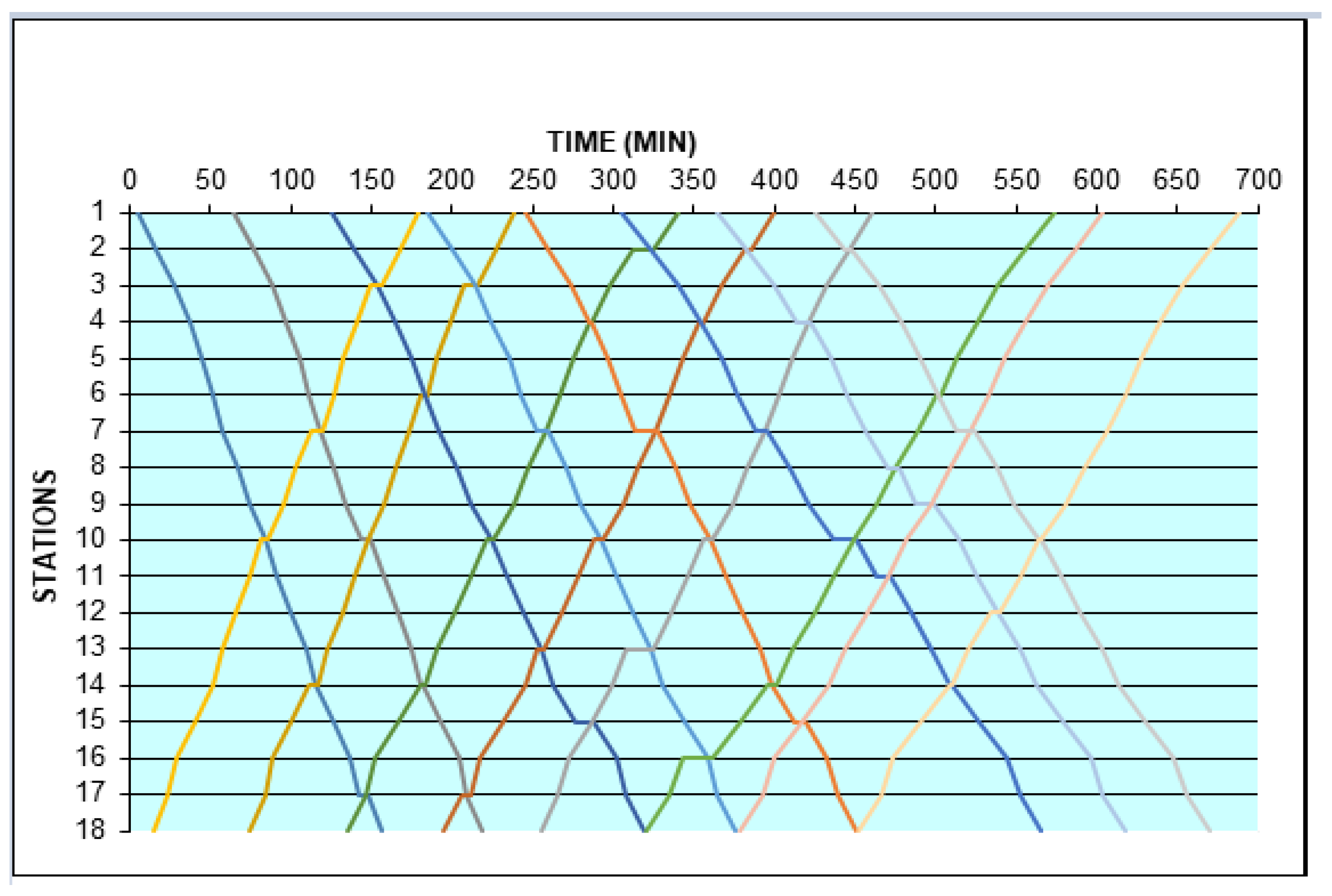
Even from the unsolved state, one can observe the simplicity of this instance. Because fast trains entered the line before slow trains, no trailing train could catch up to the train in front. Even in their smallest form, the headways between two trains in the same direction at any point were at least 60 min. This implies that no overtaking constraints and no following constraints were active. Moreover, station capacity constraints will not be active at all. Lastly, some of the trains moving in opposite directions will never meet within the line. The problem space restriction algorithm and lazy constraint attribute will recognize such special structures and make the instance even easier to solve. In Figure 4, the solved state of this special instance is shown. Unsurprisingly, this special instance was solved within only 7 s. Therefore, despite having more trains, this special instance was much easier than the 6 + 5 train instances that will be presented below.

Figure 4. The solved (optimal) state of the special 8 + 8 train instance.

Encouraged by the success in solving the 8 + 8 train special instance, we also tried a 13 + 13 problem formed with the same logic. Even the 13 + 13 train problem was solved in 80 s. This implies that a 13 + 13 instance can be easier than a 6 + 5 instance if it is specially formed. These findings suggest that the number of trains and stations cannot accurately define the difficulty of the problem instance. The frequency and entrance time order of the trains are also required to define the difficulty.

4.2.2. Minimum Running Times of Trains

A single minimum running time scheme was used for all the instances. It is given in Table 10. In the table, the number in the row of station s corresponds to minimum running time between stations s and s + 1. Hence, the row of Station 18 is empty.

Table 10. Minimum running times (minutes).

	TRAIN TYPE
Station Number	Fast	Semi-Fast	Slow
1	12	15	18
2	11	14	17
3	9	11	14
4	8	10	12
5	6	8	10
6	7	9	11
7	9	11	14
8	7	9	11
9	10	12	15
10	8	10	12
11	8	10	12
12	9	11	14
13	6	8	10
14	11	14	17
15	11	14	17
16	5	6	8
17	9	11	14
18	-	-	-

4.2.3. Recovery Times and Entrance Delays of the Trains

Every train enters the line either with some recovery time or unrecoverable delay. Therefore, the generic model accepts recovery times and initial unrecoverable delays as inputs, either explicitly or implicitly, hidden within the relation between the scheduled arrival time and the earliest possible arrival time. The earliest possible arrival time of a train is simply the sum of all minimum running times and the minimum dwell times of that train added to the entrance time of that train. Scheduled arrival time is a parameter described in Table 3.

4.2.4. Entrance Times of the Trains

Trains were introduced into the line at random times. However, the same order given in Table 4 and regarding the high frequency principle was always respected. The entrance times are given in Table 11.

Table 11. Entrance times of the trains into the system, with respect to time zero (minutes).

	Train 1	Train 2	Train 3	Train 4	Train 5	Train 6	Train 7	Train 8	Train 9	Train 10	Train 11
Instance 1	79	60	95	39	40	49	59	6	9	23	26
Instance 2	82	57	92	42	43	46	56	9	12	26	23
Instance 3	46	66	56	37	22	56	33	7	2	19	12
Instance 4	67	72	81	34	33	54	51	1	4	16	19
Instance 5	73	70	85	41	43	56	56	9	5	26	25
Instance 6	72	54	88	33	39	44	58	1	9	14	19
Instance 7	76	67	91	37	37	48	57	2	8	18	27
Instance 8	59	69	75	38	31	54	44	9	1	27	19
Instance 9	82	72	100	41	44	53	62	9	1	23	26
Instance 10	67	54	83	28	33	44	53	5	2	16	13

4.2.5. Minimum Headways between Trains

The concept of minimum headway between any successive train’s movements on a particular track element, which would be enforced by the signaling system to maintain operational safety, was adopted.

Three different minimum headways were defined: minimum arrive–arrive headway, minimum depart–depart headway and minimum arrive–depart headway. In reality, their values may be different for each train couple and each station. However, for simplicity, they were assumed to be constant in all the instances. Table 12 shows the minimum headway values.

Table 12. Minimum headways.

Min Arrive–Arrive Headway (min)	Min Depart–Depart Headway (min)	Arrive–Depart Headway (min)
2	3	2

4.3. Results of the Test Runs

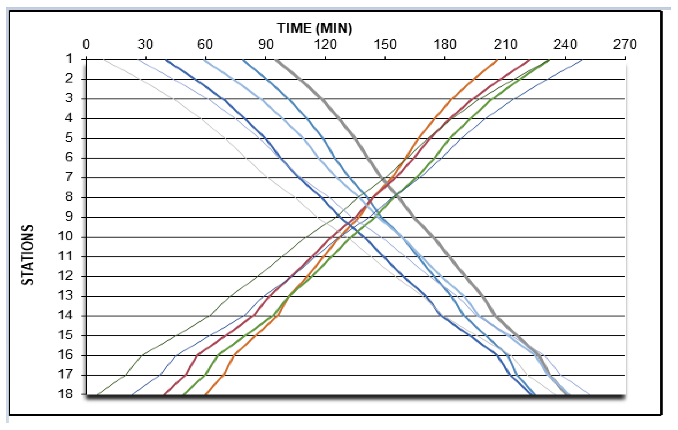
The constructed instances were run on a computer with an Intel Core i5-2400 processor with 3.1 GHz processor speed and 6.0 GB RAM. In Figure 5, the initial state of Instance 1 is given. The figure shows trains’ free paths with their minimum running times. Please note that the instance shown in Figure 5 is much more difficult to solve than that in Figure 3 because of the unfavorable entrance time orders and close entrance times.

Figure 5. Initial (infeasible) state of Instance 1.

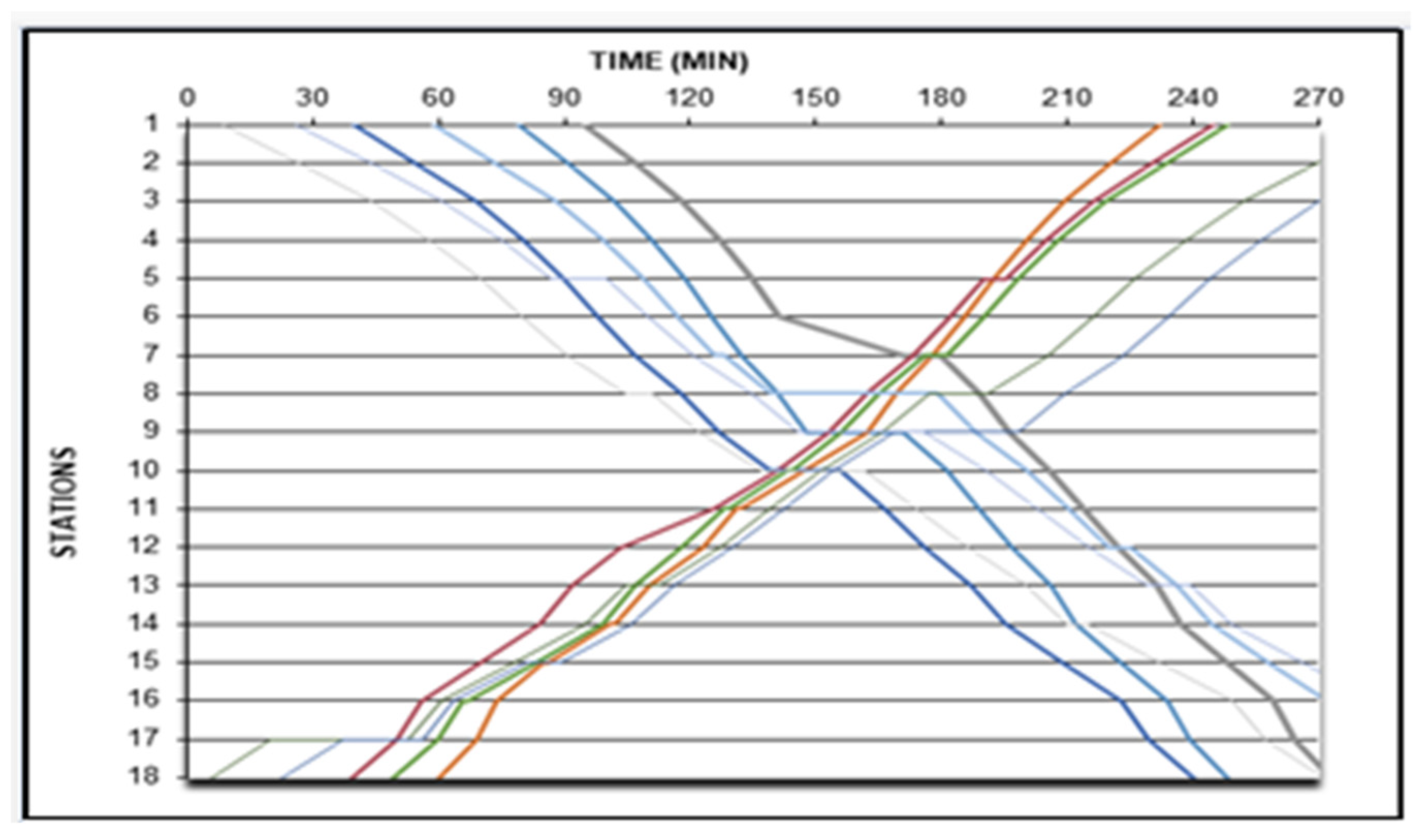
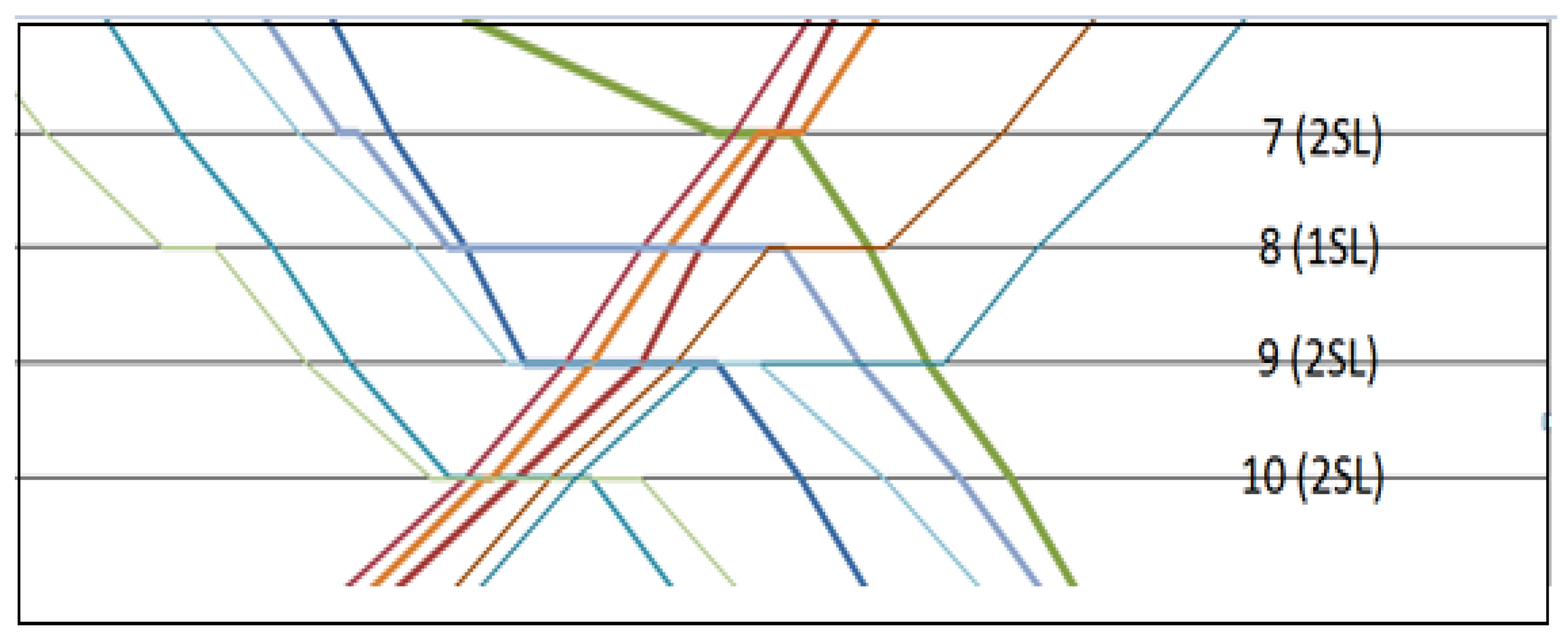
As seen in Figure 6, all conflicts are resolved. In this instance, there was a congested area between stations 7 and 10. None of the station or siding capacities were violated in the final solution. In Figure 7, the congested area in Figure 6 is zoomed in to better visualize the conflict resolutions and station track occupations. In Figure 7, the numbers of secondary lines (abbreviated as SL) in the stations are also given. As seen in this figure, no station capacity was violated in the rescheduling.

Figure 6. Final solution of Instance 1.

Figure 7. Congested area of Instance 1 is zoomed in.

In Figure 6, the final solution generated with the algorithm is presented.

In Table 13, the summary of the solution of Instance 1 is given. The results of all ten instances (together with Instance 1) are summarized in Table 14. Despite the numbers of eastbound and westbound trains being the same in every instance, there are slight differences observed in the number of binary variables created with the solution space restriction algorithm (described in Section 3.2.2). Once a decision variable is fixed, the solver treats that variable as a parameter and does not count it in the total number of variables. Lastly, the number of constraints seem to be relatively high, but very few of these constraints were actually binding at any iteration of the algorithm. Most of them were lazy constraints as defined in Section 3.2.1. They were explicitly considered only if they were violated in the LP relaxation.

Table 13. Summary of the solution of Instance 1.

Train Number	Entrance Time (min)	Arrival Time (min)	Desired Arrival Time (min)	Arrival Delay (min)	Weight	Weighted Delay (min)
1	79	248	225	23	6	138
2	60	232	206	26	6	156
3	95	273	241	32	6	192
4	39	245	222	23	4	92
5	40	240	223	17	4	68
6	49	248	232	16	4	64
7	59	289	242	47	4	188
8	6	287	232	55	3	165
9	9	271	235	36	3	108
10	23	305	249	56	3	168
11	26	305	252	53	3	159

Table 14. Summary of all the final solutions of every instance.

Instance Number	# of Binary Variables	# of Continuous Variables	# of Constraints	Max. Weighted Delay (min)	Total Weighted Delay (min)	Solution Time (s)
1	457	387	38501	192	1498	84
2	463	387	38462	192	1383	96
3	501	387	38694	198	1562	101
4	445	387	37828	195	1593	87
5	493	387	38694	204	1384	108
6	498	387	39052	198	1496	116
7	461	387	38069	198	1408	119
8	515	387	39049	201	1466	164
9	462	387	38349	192	1453	130
10	467	387	38479	204	1370	105

Experiments on a Small-Sized Problem Instance to Demonstrate the Effects of Speed-Up Methods

Due the intractable nature of train rescheduling problems, it was not possible to solve the larger sized instances in a reasonable amount of time without speed-up routines. This fact makes the observing the effects of the individual speed-up routines impossible in the largest instances. Hence, to demonstrate the effects, we set up a 4 + 4 train problem instance. In this instance, the train entrance orders and frequencies follow the same schemes with the other runs. Minimum running times, weights and minimum headways were also the same. Train orders and entrance times are given in Table 15 and Table 16, respectively.

Table 15. Train orders in the 4 + 4 train instance.

Train Numbers	Directions	Train Types	Weights
1	Eastbound	Fast	6
2	Westbound	Fast	6
3	Eastbound	Semi-fast	6
4	Westbound	Semi-fast	4
5	Eastbound	Slow	4
6	Westbound	Slow	4
7	Eastbound	Slow	4
8	Westbound	Slow	3

Table 16. Entrance times of the trains into the line in the 4 + 4 train instance with respect to time 0.

	Train 1	Train 2	Train 3	Train 4	Train 5	Train 6	Train 7	Train 8
Entrance times (min)	50	70	35	30	5	50	20	30

The instance was run using the same hardware and software as the previous instances and adopting four different approaches: no speed-up (Base), using only the lazy constraint attribute (Lazy), using the lazy constraint attribute with the solution space restriction algorithm (Lazy + Restr) and finally the multiobjective added onto the top of them (Lazy + Restr + Multi). At every minute, the optimality gaps were recorded; the results are shown in Figure 8. Figure 8 clearly displays the performance differences of the approaches. In Table 17, it can be seen what happens if the solution were not interrupted until the end (optimal solution). This table also demonstrates the effects of the speed-up routines on the problem tractability. In addition, for this instance, it can be seen that the solution restriction algorithm found the optimal solution. Given the development of the approaches in line with the railway operation practices, we concluded that this algorithm will find the optimal solution most of the time. In Table 18, the arrival time and delay data of trains in the final solution are given. The models with and without the solution space restriction algorithm produced exactly the same solution as each other. The last one naturally produced a different objective value because it was a multiobjective problem.

Figure 8. Comparison of optimality gaps for first five minutes of running.

Table 17. Outcomes of the instance with different approaches.

Instance Label	# of Binary Variables	# of Continuous Variables	# of Constraints	Total Weighted Delay (min)	Computation Time (s)
Base	634	281	12,164	707	1156
Lazy	634	281	12,164	707	711
Lazy + Restr.	298	281	11,073	707	93
Lazy + Restr + Multi	298	281	11,081	797	3

Table 18. Summary of the optimal solution of the 4 + 4 instance.

Train Number	Entrance Time (min)	Arrival Time (min)	Desired Arrival Time (min)	Arrival Delay (min)	Weight	Weighted Delay (min)
1	50	208	188	20	6	120
2	10	228	211	17	6	102
3	35	252	213	39	4	156
4	30	245	231	14	4	56
5	5	248	229	19	3	57
6	50	263	235	28	3	84
7	20	278	245	33	3	99
8	70	266	255	11	3	33

5. Discussion and Conclusions

In this study, we aimed to develop a MILP model for rescheduling train traffic on a single-track railway line. This model takes into account the station and siding capacity constraints by enumeration. The train scheduling problem is an NP-complete problem with a structure similar to an extremely difficult version of the job–shop scheduling problem. The combinatorial structure of this problem dominated all of the trial runs. Without any heuristic improvement, the solver could solve only small instances, e.g., a 3 + 3 train problem (three eastbound plus three westbound trains). However, all of the heuristic improvements helped to increase this number to, for now, 6 + 5 trains. The algorithm could solve a 6 + 5 train problem within a duration of less than three minutes. This is a considerable improvement. In real operations, rescheduling problems have to be solved in a very short time because they have to be solved in a dynamic environment. The model treats the trains as static entities, but in reality, they would be moving. Note that the instances were chosen carefully to be as difficult as possible. Normally, railway authorities tend to “speed-fleet” the trains in timetabling. That means trains in the same direction enter the line segment in the order of decreasing speed, thus minimizing the number of potential following and overtaking conflicts. However, in our instances, the scheme is just the opposite. Trains were introduced into the line in the order of increasing speed, thus maximizing the potential following and overtaking conflicts. Trains were introduced into the system with headways from 10 to 20 min/train/direction, which is indeed an unrealistically high train frequency for such a long (18 stations, approximately 160 km) single-track line. This unrealistically high frequency of trains was, again (like the difficulty created in choosing the order of trains), chosen for observing some kind of worst-case performance [1].

The solution space restriction algorithm shortened the solution time of the model quite radically. Indeed, in its presolve stage, CPLEX applies its own algorithms to eliminate some of the constraints and variables. However, we can be more aggressive in elimination because our algorithm is indeed based on a solution of the problem, albeit a relaxed version (station and siding capacities). Because this algorithm reduces the number of possible meeting locations, it is not possible to provide formal proof of the optimality of the solutions. However, based on our own knowledge and experience in railway operations, we can argue that, in the optimal solution, it is highly unlikely that the meeting will need to be outside the region defined by this restriction algorithm. In the trials, the length of this region was five stations. Carrying the meeting point outside of this region creates an excessive waiting time for one of the trains, and this most probably contradicts with the maximum weighted delay objective.

The multiobjective approach provided a surprisingly good boost for solution speed. It provided on the order of 90% improvement in the computation time. In the trial runs, it was observed that most of the time was consumed by the first problem, the minimum–maximum weighted delay. After the solution of the first problem, the second and major problem were indeed very quickly solved in only a few seconds. This was most probably due to the properties and capabilities of CPLEX. Both problems have the same feasibility domains, thus any combination of decision variable values that is feasible for one problem is also feasible for the other. Most probably, CPLEX can improve the solution with simple time shifts and quickly arrive at the optimal solution. Because the problem was solved in a heuristically restricted solution space, it is not possible to present a formal proof of optimality. However, at least the modeling approach was designed towards obtaining a Pareto-optimal solution because the problem was converted into a multiobjective one. However, this is not a very typical multiobjective problem. There is a slight contradiction between the objectives (see Table 2), and additionally, a positive correlation exists. The positive correlation between two objectives may have also helped increase the solution speed.

6 + 5 trains may seem to be a small problem instance, but in reality, it is not. Rescheduling algorithms have to be run in dynamic environments. Trains are moving, and they can always gain additional primary delays. This necessitates the model to be rerun several times. This puts a practical limit to the time horizon of a rescheduling problem. Time horizon is a preset limit to the scope of the rescheduling problem. In the literature on rescheduling, quite narrow time horizons (e.g., less than one hour) are commonly found. In this study, the length of the time horizon was, however, more than two hours from initial departure time of the first train to the resolution of the last conflict (See Figure 6). Furthermore, as previously stated, we tested our algorithm on instances with relatively short headways for a single-track railway, averaging between 10–20 min in one direction, to see the worst-case performance of the algorithm. In addition, in these instances, we introduced the trains into the system in an order that maximized the number of following and overtaking conflicts. To the best of our knowledge, no other study analyzes such a worst-case performance. Thus, 6 + 5 is quite a high number of trains to be rescheduled on a single-track railway line, given the worst case approach (small headways and order of the trains specially chosen to maximize the number of intertrain conflicts to be resolved) used. Lastly, we considered quite a long stretch of a single-track railway, with 17 stations included. Recent entries in the literature have been generally focused on double-track lines in which there are no meetings and the number of secondary lines is not a major problem, often not considered at all. However, there are still single-track railways all over the world. We consider these facts as the significance and contribution of our study.

Like all studies in this field, our study has some limitations, assumptions and simplifications. Conflict resolution often brings unplanned stops to some trains, and these increase minimum running times due to the typically slow acceleration and braking capabilities of rail vehicles. Our model assumes that minimum running times are independent from acceleration and braking. Indeed, acceleration and braking effects are partially and implicitly reflected in the numerical values of the minimum headways. Moreover, in most cases, waiting times (due to conflict resolutions) are a lot longer than the running time increases that acceleration and braking can cause; therefore, we conclude that this limitation would not be a real performance deficit. We note that, on the other hand, neglecting time losses due to acceleration and braking is quite a common practice in the literature, as incorporating them makes the underlying mathematical model nonlinear. Another limitation of the study is its pure focus on rescheduling. Although we present a generic model that can be extended to train scheduling at a tactical level (timetabling), this is not the main purpose of the study. The study was designed with rescheduling in mind. Therefore, no timetable was prepared in the process, and no timetable quality factors (e.g., meeting the passenger or freight demand, periodicity, obedience to the desired train timing intervals, timetable robustness, energy efficiency, etc.) have been considered. We did not consider other tactical planning issues such as crew scheduling, rolling stock scheduling, etc. One of the unique features of our study is that we used a two-objective model, i.e., trying to minimize both the weighted maximum delay and the weighted total delay. Minimizing delays over such objectives would certainly help avoid losing feasibility in rolling stock circulation and crew circulation.

Future work on this model will include adopting cleverer decomposition algorithms. In our mathematical model, we defined meetings in stations with more than one secondary track by two binary variables per station per train couple. This puts a huge computational workload onto the model, and it was unnecessary most cases. Such variables are needed only when siding capacity constraints for more than one eastbound train and more than one westbound train will be binding at a particular station. Thus, future work will include such decomposition algorithms that these variables may also be “lazy”.

References

1. Aydın, G. Planning of Train Movements in Single Track Railways. Ph.D. Thesis, Yıldız Technical University, Istanbul, Turkey, September 2015. Thesis No: 406540. Available online: https://tez.yok.gov.tr/UlusalTezMerkezi/giris.jsp (accessed on 28 December 2022).
2. Veelenturf, L.P.; Kidd, M.P.; Cacchiani, V.; Kroon, L.G.; Toth, P. A railway timetable rescheduling approach for handling large-scale disruptions. Transp. Sci. 2016, 50, 841–862. [Google Scholar] [CrossRef]
3. Sels, P.; Dewilde, T.; Cattrysse, D.; Vansteenwegen, P. Reducing the passenger travel time in practice by the automated construction of a robust railway timetable. Transp. Res. Part B Methodol. 2016, 84, 124–156. [Google Scholar] [CrossRef]
4. Taslimi, B.; Babaie Sarijaloo, F.; Liu, H.; Pardalos, P.M. A novel mixed integer programming model for freight train travel time estimation. Eur. J. Oper. Res. 2022, 300, 676–688. [Google Scholar] [CrossRef]
5. Samà, M.; Pellegrini, P.; D’Ariano, A.; Rodriguez, J.; Pacciarelli, D. Ant colony optimization for the real-time train routing selection problem. Transp. Res. Part B Methodol. 2016, 85, 89–108. [Google Scholar] [CrossRef]
6. Šemrov, D.; Marsetič, R.; Žura, M.; Todorovski, L.; Srdic, A. Reinforcement learning approach for train rescheduling on a single-track railway. Transp. Res. Part B Methodol. 2016, 86, 250–267. [Google Scholar] [CrossRef]
7. Liu, L.; Dessouky, M. A decomposition based hybrid heuristic algorithm for the joint passenger and freight train scheduling problem. Comput. Oper. Res. 2017, 87, 165–182. [Google Scholar] [CrossRef]
8. Ait-Ali, A.; Lindberg, P.O.; Eliasson, J.; Nilsson, J.E.; Peterson, A. A disaggregate bundle method for train timetabling problems. J. Rail Transp. Plan Manag. 2020, 16, 100200. [Google Scholar] [CrossRef]
9. Josyula, S.P.; Törnquist Krasemann, J.; Lundberg, L. A parallel algorithm for train rescheduling. Transp. Res. Part C Emerg. Technol. 2018, 95, 545–569. [Google Scholar] [CrossRef]
10. Gao, R.; Niu, H. A priority-based ADMM approach for flexible train scheduling problems. Transp. Res. Part. C Emerg. Technol. 2021, 123, 102960. [Google Scholar] [CrossRef]
11. Sinha, S.K.; Salsingikar, S.; SenGupta, S. An iterative bi-level hierarchical approach for train scheduling. J. Rail Transp. Plan Manag. 2016, 6, 183–199. [Google Scholar] [CrossRef]
12. Bettinelli, A.; Santini, A.; Vigo, D. A real-time conflict solution algorithm for the train rescheduling problem. Transp. Res. Part B Methodol. 2017, 106, 237–265. [Google Scholar] [CrossRef]
13. Şahin, İ. Railway traffic control and train scheduling based on inter-train conflict management. Transp. Res. Part B Methodol. 1999, 33, 511–534. [Google Scholar] [CrossRef]
14. Filcek, G.; Asior, D.; Hojda, M.; Józefczyk, J.; Filcek, G.; Asior, D.; Hojda, M.; Józefczyk, J. An Algorithm for Rescheduling of Trains under Planned Track Closures. Appl. Sci. 2021, 11, 2334. [Google Scholar] [CrossRef]
15. Tiong, K.Y.; Palmqvist, C.-W.; Olsson, N.O.E. The Effects of Train Passes on Dwell Time Delays in Sweden. Appl. Sci. 2022, 12, 2775. [Google Scholar] [CrossRef]
16. Martin-Iradi, B.; Ropke, S. A column-generation-based metaheuristic for periodic and symmetric train timetabling with integrated passenger routing. Eur. J. Oper. Res. 2022, 297, 511–531. [Google Scholar] [CrossRef]
17. Högdahl, J.; Bohlin, M.; Fröidh, O. A combined simulation-optimization approach for minimizing travel time and delays in railway timetables. Transp. Res. Part B Methodol. 2019, 126, 192–212. [Google Scholar] [CrossRef]
18. Sparing, D.; Goverde, R.M.P. A cycle time optimization model for generating stable periodic railway timetables. Transp. Res. Part B Methodol. 2017, 98, 198–223. [Google Scholar] [CrossRef]
19. Cavone, G.; Dotoli, M.; Epicoco, N.; Seatzu, C. A decision making procedure for robust train rescheduling based on mixed integer linear programming and Data Envelopment Analysis. Appl. Math. Model. 2017, 52, 255–273. [Google Scholar] [CrossRef]
20. Li, W.; Ni, S. Train timetabling with the general learning environment and multi-agent deep reinforcement learning. Transp. Res. Part B Methodol. 2022, 157, 230–251. [Google Scholar] [CrossRef]
21. Samà, M.; Meloni, C.; D’Ariano, A.; Corman, F. A multi-criteria decision support methodology for real-time train scheduling. J. Rail Transp. Plan Manag. 2015, 5, 146–162. [Google Scholar] [CrossRef]
22. Altazin, E.; Dauzère-Pérès, S.; Ramond, F.; Tréfond, S. A multi-objective optimization-simulation approach for real time rescheduling in dense railway systems. Eur. J. Oper. Res. 2020, 286, 662–672. [Google Scholar] [CrossRef]
23. Törnquist, J.; Persson, J.A. N-tracked railway traffic re-scheduling during disturbances. Transp. Res. Part B Methodol. 2007, 41, 342–362. [Google Scholar] [CrossRef]
24. Acuna-Agost, R.; Michelon, P.; Feillet, D.; Serigne, G. A MIP-based Local Search Method for the Railway Rescheduling Problem. Networks. 2011, 57, 69–86. [Google Scholar] [CrossRef]
25. Törnquist Krasemann, J. Design of an effective algorithm for fast response to the re-scheduling of railway traffic during disturbances. Transp. Res. Part C Emerg. Technol. 2012, 20, 62–78. [Google Scholar] [CrossRef]
Disclaimer/Publisher’s Note: The statements, opinions and data contained in all publications are solely those of the individual author(s) and contributor(s) and not of MDPI and/or the editor(s). MDPI and/or the editor(s) disclaim responsibility for any injury to people or property resulting from any ideas, methods, instructions or products referred to in the content.
Article Metrics
Citations
Article Access Statistics
Multiple requests from the same IP address are counted as one view.