Abstract
The operational measure (OM) of the Second-Generation Intact Stability Criteria (SGISC) is the initial step toward the design of a performance-based dynamic stability assessment of the ship by considering the vessel’s operation, loading condition and weather parameters. The SGISC recommends the standard wave scatter table (WST) for the environmental data, an indefinite requirement for a simplified assessment pathway, which provides the probability of wave occurrence. The existing standard WST was developed based on the North Atlantic Ocean. The study aims to identify the discrepancy in the probability of wave occurrence in the IMO-recommended WST when compared with developed hindcast WST for smaller regions of the North Atlantic Ocean for the application of the SGISC. This study is one of a kind and very significant, given that the assessment using the standard WST provided unrestricted operational ability to ship under the SGISC. The findings of this research provide insights into significant differences in the existing standard WST when compared graphically with hindcast data, especially across different seasons of the North Atlantic Ocean. A case study of OMs on the C11 class post-Panamax container ship for excessive acceleration is provided to better represent the study. In the case study, the operational limitation defined by the hindcast WST for individual sea areas and seasons is compared with the standard WST. This investigation shows that regional and seasonal operational limitations are required for season 4 operation beyond the standard WST safety estimation and that the operational limitation achieved with standard WST is not adequate. The findings suggest that the identified limitations significantly limit the use of a standard WST for unrestricted operational validation in the SGISC. The provided recommendation is very relevant in improving the safety assessment using vulnerability criteria, given that the hindcast data are reliable and available for the season and are also region-specific, and hence the accuracy of the ship stability can be improved while using the SGISC.
1. Introduction
The Second-Generation Intact Stability Criteria (SCISC) are used for the dynamic design stability assessment of a ship, are endorsed and adopted by the International Maritime Organisation (IMO), and were finalised at the seventh session of the (IMO) sub-committee, which was held in February 2020 [1]. A final draft of the explanatory notes for evaluating the ship using the SGISC is a working process [2] and is delayed due to the COVID-19 outbreak. In the SGISC, a three-tier assessment pathway is defined, with increased complexity on assessment down the pathway, namely vulnerability criteria one (VC1) (vulnerability criteria one is the simplest stability assessment method available in the SGISC), vulnerability criteria two (VC2) (vulnerability criteria two is the simplest probabilistic stability assessment pathway in the SGISC) and direct stability assessment for five-ship dynamic failure modes. Each path in the SGISC is independent; thus, successful validation of the ships using any individual path is acceptable. The SGISC also addresses the operational aspect through operational measures with the above pathways: simplified operational measures using VC1 and VC2; and probabilistic and deterministic operational measures using the direct stability assessment pathway. The operational measure encompasses operational limitation and operational guidance, where the former limits the conditions in which a ship can operate if it fails to meet the safety standard, while the latter recommends operating parameters for conditions limited by the former [1,3].
All design assessment pathways in the SGISC require three input factors: the environmental factor, the ship’s internal loading conditions and the ship’s design parameters. The environmental condition is the most challenging among the considered input factors, especially when developing operational measures (OMs). Accurate environmental data are required to identify operational limitations and operational guidance parameters. Meanwhile, a simplified OM uses a wave scatter table (WST), which is a collection of historical wave data statistics. The SGISC provides no specific directions to incorporate real-time weather data while using the WST for effective OMs [4]. The WST provides the probability of wave occurrence as a function of significant wave height and zero-crossing period. The SGISC recommends using the standard WST (Figure 1) to assess the dynamic behaviour of a ship [1].
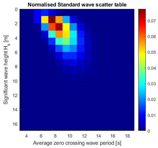
Figure 1.
Existing standard WST (sea areas 8, 9, 15 and 16).
BMT UK provides the WSTs for 104 sea areas, as shown in Figure 2 [5,6,7], including four seasons annually. However, the WSTs are not available for all seasons and all sea areas defined in the globe. The individual WST for the regions and seasons is an example of a local WST. The WST is based on visual observations of the wave’s relative motion with respect to the ship’s direction, which is reported to the Main Marine Databank of the UK Meteorological Office from ships operating in specific regions. The data are collected randomly at different conditions by different observers over the years. It is worth mentioning that standard WST only covers sea areas 8, 9, 15 and 16, as defined in [8]. The stored wave data are quality controlled and enhanced by the well-validated NMIMET method. The NMIMET method takes into account swell, but the wave period estimates are expected to be less reliable in areas where the swell is a major component of the climate (such as in tropical regions) [8]. In addition, the data do not reflect on areas prone to typhoons or hurricanes, as it is unlikely for a visual observation to be obtained of this region because ships are operated to avoid regions of rough sea. These limitations are barriers to estimating a reasonably acceptable ship’s dynamic behaviour using the simplified SGISC. The following paragraph outlines the application of the standard and the modified WSTs on the simplified OM assessment of the SGISC.
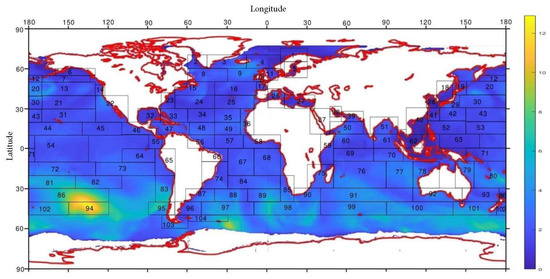
Figure 2.
Sea area nomenclature with hindcast significant wave height snapshot.
The pathway to estimate ship stability using vulnerability criteria and simplified operational measures is addressed in [1,4] and [3], respectively. Similar to the three independent pathways of assessment, any combination of simplified operational measures outlined below could be used independently for assessing the ship’s stability for each failure mode. For a ship to have unrestricted operation, the ship must pass the threshold criteria laid out in the SGISC without operational measures. The ship which fails to meet the threshold criteria with the standard WST can use a modified WST, limiting the operation to the modified WST’s location, route, or season. Further, the operational limitations could be defined at a specific significant wave height for the standard WST or modified WST based on a given SGISC assessment. This process limits the operation of the ship to a defined significant wave height across the globe if assessed against the standard WST or restricted to the modified WST’s region, route, or season. However, in the case of failure to achieve a successful combination with operational limitations, the ship can operate with the operational guidance based on the modified or the standard WST if the design assessment is accepted. This allows the ship to operate with the operational parameters advised. The above combination of operational limitation and operational guidance is only accepted if the ship’s total operation failure time to the total ship operation time estimated based on the standard or modified WST is less than 0.2 for the considered operation limitation and operation guidance [1,3].
Therefore, the operational time for a ship considering an individual wave is important in estimating acceptance criteria and is defined by the magnitude of the probability of occurrence of the wave in the WST. The total operational time is the summation of individual operating time in encountering each wave case with non-zero probability in the WST. The change in the WST will result in a change in the probability distribution of wave occurrence and hence the operating time. Thus, the individual operating time of the ship in encountering each wave varies with different WSTs. On the other hand, changing the WST according to region, season and route gives a more accurate reading of wave probability with respect to time and location [4,9]. By doing so, the OM will be defined based on the actual operating condition, i.e., the region and seasonal circumstance; thus, using the modified WST improves the accuracy of weather data and furthers the accuracy of design assessment. Therefore, it is vital to verify the representation of the wave and its probability of occurrence in the WST used for the SGISC assessment. This paper investigates the existing standard WST representation of the wave profile when compared to individual sea areas. The investigation compares the quality and representativeness of waves in the recommended standard WST with the hindcast data WST and compares OM outcomes for both region and season. The novelty of this paper appears in investigating the need for regional and seasonal WST over the standard WST.
The use of real-time weather data is a different approach compared to intact stability regulations given in the 2008 IS Code [10]. It allows for achieving real-time operational stability using SGISC. Two factors are considered important to achieve the required assessment: real-time weather data and ship operation status. The forecasted WST can be used for the ship operation guidance if data are available for number of days. Therefore, real-time ship stability analysis during operation will emerge as a systematic, regulated and recognised approach [11].
A review of the SGISC specifically on OMs and subsidiary topics can be found in Shigunov et al. [12], and there is an increasing number of publications on OMs [13,14]. A significant amount of research is in progress to regulate the practical application of simplified operational measures, some of which includes studies addressing operational limitations based on the standard WST or modified WST for specific failure modes and ship types [15,16,17]. Studies are also being conducted on the application of guidance [18,19]. In addition, some research focuses on variation in stability estimation when different weather data sources are used [20,21]. Meanwhile, other studies used a numerical approach by incorporating operational limitations [22] and route navigation simulations to assess the failure modes and using ship-traffic-based AIS data [23]. However, the limits on the recommended standard WST are not assessed, given that successful validation with the same will achieve ships with unrestricted operation. Therefore, it is important to assess the recommended standard WST’s safety limit that holds valid for major seasons and regions. However, such a study is not available, and, therefore, is carried out in this paper using hindcast data. The study allows to identify the existing limitation of the standard WST.
2. Methodology
In this section, the methodology is discussed by looking at the technique used for developing the local/modified WST, followed by the comparative study of the WSTs. The discussion extends to analysing the excessive acceleration operational limitation.
2.1. Developing Hindcast WST
Australian meteorological hindcast data were used to develop standard and local/seasonal WSTs for sea areas under consideration, i.e., the North Atlantic Sea, given that hindcast data are the most reliable source for historical weather data analysis. The Bureau of Meteorology (BoM), Australia, and the CSIRO have developed a hindcast model called the Centre for Australian Weather and Climate Research Wave Hindcast (CAWCR), which uses WAVEWATCH III, a numerical model, to provide higher-resolution global meteorological data. The model has been well-validated and updated over the years [24]. It has undergone two updates in the past, and since June 2013, no significant configuration change has been made to the model. The data available have 0.4-degree spatial and hourly temporal resolution for the global data. The spatial resolution is higher for the region around Australia. For this study, the data from June 2013 to March 2022 with a spatial resolution of 0.4 degrees are used. The CSIRO provides free access to the hindcast model through the CSIRO data server. The server is populated monthly with the previous month’s hindcast file [7].
The monthly files (netCDF file format) required for the study were downloaded to the local system and striped for parameters shown in Table 1 for the North Atlantic Sea. The temporal data of the North Atlantic Sea area were saved under individual sea area numbers, i.e., 8, 9, 15 and 16, to reduce the size of individual files. To further reduce the size of the file and for fast processing, each monthly sea area file was reduced to a monthly WST for wind, swell and mean sea using an in-house-developed algorithm. The algorithm is capable of developing WSTs for customised sea regions, including customised time for wind, swell and mean sea. The individual monthly WST is a 25 by 25 matrix and is stored in a structured format to m.files, which is used for further analysis in this study. The data set developed is a simple way of looking into the sea state contribution of swell, wind and mean sea.

Table 1.
Developed WST hindcast file parameters.
The monthly data are sorted as a function of wave height and zero-crossing wave period, and the occurrence of each state is counted to the respective matrix (mean, wind and swell). The matrix has unit meter and unit period resolution. The following data points are considered for generating a WST: significant wave height (hs) and mean period of first frequency moment (t01), significant wave height of wind sea (phs0) and peak period of wind sea (ptp0) and significant wave height of primary swell (phs1) and peak period of primary swell (ptp1). The combinations of the above parameters make the mean sea WST, the wind sea WST and the swell sea WST as given in Table 1. Equations (1) and (2) are used to estimate the zero-crossing wave period, since it is not directly available from the peak and mean wave period. The CAWCR wave model uses the JONSWAP wave model to develop the hindcast wave model [7]. The developed matrix is called the local hindcast WST.
where Tz is the zero-crossing period, T1 is the mean period, Tp is the peak period and γ is the peak shape parameter (γ = 3.3).
From the monthly local hindcast WST, the annual and seasonal WSTs are developed by summing the monthly WST for respective months. The seasonal and annual WSTs are then summed up to consecutive 2-, 5- and 10-year WSTs to investigate the sea state variation over the years. The sample size of the wave in each WST is different due to differences in the size of each sea area and also the temporal sampling length for each developed WST. Subsequently, the annual and seasonal WSTs are normalised such that the cumulative probability of occurrence of each table is one for better comparison, as shown in Table 2. In this study, the 10-year data set is used, which is more appropriate for research that requires regional and seasonal WSTs.
Table 2.
File names.
2.2. WST Comparison
For the comparison study of the WSTs, the probability of wave occurrence is summed with respect to wave height to plot the probability density function (pdf) vs. wave height for each WST. In order to carry out a quick comparison of WSTs regarding the regional and seasonal WSTs, each WST’s pdf corresponding to the Rayleigh pdf function is mapped, and the Rayleigh shape parameter () is compared to identify the variation in WSTs. To carry out the mapping of the Rayleigh pdf to match the hindcast WST’s pdf, the following three techniques were used: (i) least square error method (LSE), (ii) least area error method (LAE) and (iii) least square error method for the peak of the curve (LSEP). The peak of the curve is the region above the mean probability of exceedance (MPoE) calculated using Equation (3). The smaller Rayleigh shape parameter means the spread is narrow with a sharp peak located closer to the lower wave height, while the larger shape parameter means the pdf is broad and flat and the peak of the pdf is towards the higher wave height.
2.3. Excessive Acceleration Vulnerability Assessment and Operational Limitation
In this study, excessive acceleration VC1 [1] is used to estimate the acceleration of a C11 class post-Panamax container ship against each WST considered for this study, which are seasonal and regional WSTs of sea areas 8, 9, 15 and 16. In detail, excessive acceleration assessment is provided by Shin and Moon using vulnerability criteria [25]. This study also incorporates the operational limitation methodology proposed by Bulian and Francescutto [26] for dead ship VC1. The methodology defined is applicable to all ship types assessed using VC1 or VC2. In Bulian’s study, the wave steepness table was updated based on the WST to introduce operational limitations to the level one dead ship condition. The same methodology is used for level one excessive acceleration estimation. The details of Bulian’s methodology are available from the reference paper, but the outline of the methodology used for this study is provided below.
The step for the excessive acceleration VC1 operational limitation:
- a.
- Define the respective WST.
- b.
- Estimate the mean wind speed for the WST at the probability of exceedance = 1.2%. For IMO’s recommended standard WST, the wave height and mean wind speed () at 1.2% probability of exceedance are 8.9 m and 26 m/s, respectively.
- c.
- Determine the modified wave steepness using Figure 3 and Equation (4) [26].
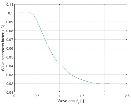 Figure 3. Wave age at natural roll period based on standard wave steepness table.
 - d.
- Apply excessive acceleration vulnerability criteria one with the modified wave steepness table.
Using the modified wave steepness table, excessive acceleration for the C11 container ship was estimated for comparison. The results of level one excessive acceleration operational limitation were compared with the example provided in Appendix 2 of the IMO SGISC draft explanatory notes [2].
where is wave age at natural roll period, Vw is mean wind speed and Tr is natural roll period.
3. Sample Ship
The C11 class post-Panamax container ship is used for this study. The inputted data are from information available on the IMO example case study and hence appropriate to compare the algorithm developed in this study. The following table provides information required for the VC1 excessive acceleration estimation (Table 3) [2].
Table 3.
C11 class post-Panamax container ship characteristics.
4. Results and Discussion
The discussion of the results in the following section is outlined in two sections. The first section validates and compares the hindcast data with the BMT global statistic data to provide insight into the outcome of the WST comparison. The second section discusses the outcome of the operational limitations using VC1 excessive acceleration.
4.1. WST Comparison
There are two sets of data used in this study: the BMT global statistic WST (hereafter BGW) [5] and the WST developed from the Australian hindcast model (hereafter AHD). In addition, we have the standard WST recommended in the SGISC interim guidelines [1], which is similar to the BGW data as it originated from BGW [8]. Figure 1 shows the standard WST recommended by the SGISC. Figure 4, Figure 5 and Figure 6 show the WST developed with hindcast mean, wind and swell sea data for the standard WST region (sea areas, 8, 9, 15 and 16, further referred together as sea area S). All WST images are normalised for comparison.
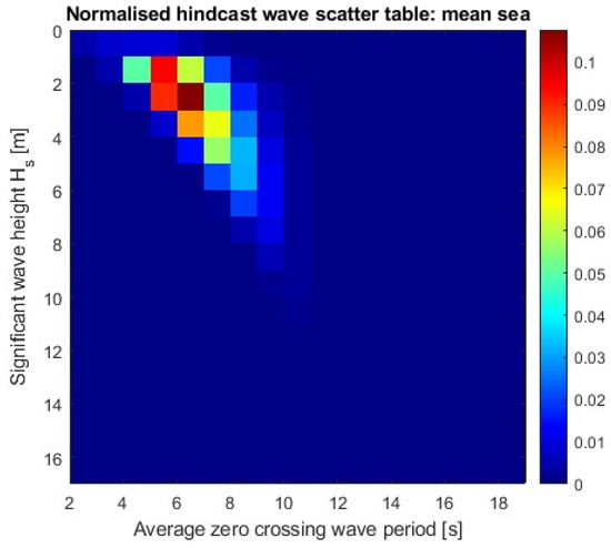
Figure 4.
Hindcast WST for mean sea (sea area S—full year).
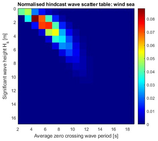
Figure 5.
Hindcast WST for wind sea (sea area S—full year).
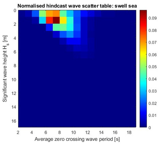
Figure 6.
Hindcast WST for swell sea (sea area S—full year).
Figure 7 shows the pdf of the standard WST provided in the SGISC, along with the associated Rayleigh pdf, and Figure 8 shows the same for sea area S using the AHD mean sea state. It is evident from Figure 7 and Figure 8 that the AHD mean sea pdf and standard WST pdf in the SGISC are almost similar for the sea area S. Additionally, the Rayleigh shape parameter for individual sea areas and sea area S is estimated using BGW, AHD mean sea, AHD wind sea and AHD swell sea data and are provided for comparison in Table 4. The statistical comparison of Table 4 is provided in Table 5. It is clear that the BGW has the highest mean shape parameter followed by AHD mean, AHD wind and AHD swell (Table 5). This shows that the assessed sea areas are wind dominant rather than swell dominant, and the trend of the sea state across all sea areas is the same, as the standard deviation is small. Hence, the evaluation of the SGISC with the standard WST is acceptable for all regions considered. Figure 9 shows the AHD swell sea state pdf, an example of a lower Rayleigh shape parameter.
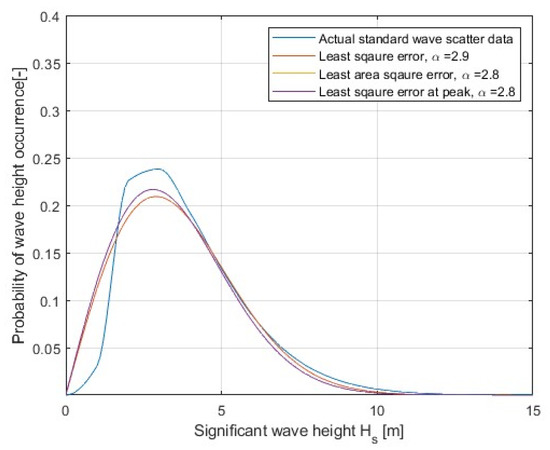
Figure 7.
Plots of standard WST pdf.
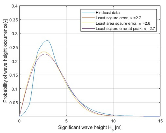
Figure 8.
Plots of WST mean sea pdf (sea area S—full year).
Table 4.
Rayleigh shape parameter for full year.
Table 5.
Statistical comparison of Rayleigh shape parameter for mean, wind and swell sea pdf (sea area S—full year).
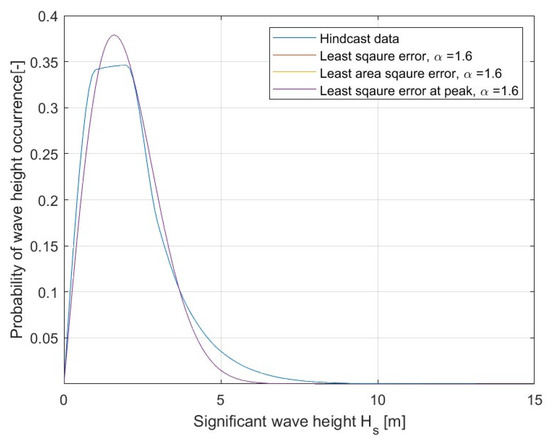
Figure 9.
Plots of WST swell sea pdf (sea area S—full year).
Similarly, for all sea areas, the seasonal WST was compared using the same technique. For this discussion, the AHD mean sea data were considered. Table 6 shows the Rayleigh shape factor comparison of WSTs for seasons 1 to 4. The statistical comparison of Table 6 is provided in Table 7, which shows that the mean Rayleigh shape factor varies over the seasons, with the highest value in season 4 and the lowest in season 2. The percentage change in the shape factor with respect to the average shape parameter of the standard WST recommended by IMO (S%) is provided in Table 7. The percentage change (S%) shows the deviation in the shape parameter for the seasonal WST from the IMO recommended standard WST shape parameter estimated in Table 5. The highest shape factor for the sea area is observed in sea area 9 for season 4, which is 49% higher than standard WST (Table 6 and Figure 10). This shows that the sea area S goes through different wave profiles during each season. The effect would be much greater if the analysis was carried out on monthly intervals instead of being seasonal. The higher shape factor for season 4 indicates that the WST of season 4 has a higher probability of occurrence for larger wave heights compared to other seasons. It is clear that in Figure 10, the peak significant wave height has increased and moved to 5 m from 3 m when comparing with Figure 7. This illustrates a significant difference among seasonal WST; hence, merging seasonal and regional sea areas will result in an inaccurate depiction of the sea profile for SGISC application. Thus, the SGISC estimation using the seasonal WST must be carried out to understand the significance of the probability of wave occurrence in different seasons. The following section is the case study of using the seasonal WST for excessive acceleration estimation. Since the standard WST is modified to the seasonal WST, the following is an example of seasonal and regional operational limitation estimates for the excessive acceleration using vulnerability criteria one.
Table 6.
Rayleigh shape parameter for AHD data (mean sea).
Table 7.
Statistical comparison of Rayleigh shape parameter for seasons 1, 2, 3 and 4.
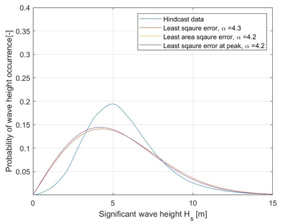
Figure 10.
Plots of WST mean sea pdf (sea area 9—season 4).
4.2. Excessive Acceleration Level One Operational Limitation
To this end, it is clear that WST varies significantly over the season for the considered sea area, hence the probability of wave occurrence. Therefore, this variation could negatively affect the estimation of simplified OM, given that the modification of environmental factors is possible in achieving OM using VC1 and VC2. In this study, Bulian methodology, as discussed in Section 2.3, is used to introduce operational limitations for evaluating excessive acceleration level one for C11 container ships. In the following discussion, only mean sea AHD data are considered, and a similar comparison could be made with AHD wind data. Table 8 and Table 9 show the estimated wave height and wind speed for developed WST based on Bulian’s method. The standard WST’s wave height and wind speeds are 8.9 m and 26 m/s (green font) [26]. The values of the same parameters for the AHD estimate, which are higher than the standard WST, are highlighted in red. Based on the developed table (Table 8 and Table 9), the wave steepness table was developed for each WST to introduce seasonal and regional operational limitations. The wave steepness factor for the standard WST recommended by IMO (Figure 11), mean AHD data sea area S full year (Table 10) and mean AHD data sea area S season 4 (Table 11) are given. It is clear that the wave steepness factor has changed significantly. With the modified WST and wave steepness factor, the excessive acceleration of C11 was estimated using the VC1 equation outlined in Section 2.3.1 of IMO SGISC guidelines [1].
Table 8.
Significant wave height (m) at probability of exceedance 1.2%.
Table 9.
Mean wind speed (m/s) corresponding to significant wave height estimated in Table 8.
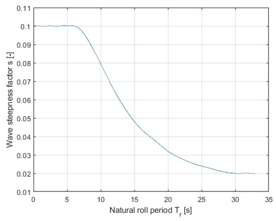
Figure 11.
Standard wave steepness table.
Table 10.
Wave steepness table AHD data (full year).
Table 11.
Wave steepness table AHD data (season 4).
To quantify the difference in using individual WSTs, the estimated excessive acceleration is compared to the example provided in [2]. Table 12 shows the estimated acceleration for the C11 container ship. It is apparent that the acceleration estimated by the standard WST is less compared to season 4 results. The excessive acceleration provided in [2] is highlighted in green. In all the WST cases considered in Table 12, the ship is vulnerable to excessive acceleration, since the estimated value is above the maximum limit of 4.64 m/s2. Let us assume that 8.1 m/s2 is the cut-off for excessive acceleration for the following discussion. The ship assessed using the standard WST will successfully pass the level one assessment and be allowed to operate unrestricted. However, the same ship which is allowed to operate in all sea areas and seasons failed the season 4 for sea area 9 assessment, which contradicts the stability results estimated with the standard WST. This demonstrates the necessity of using local and regional WSTs rather than a universal WST for the SGISC stability assessment to avoid misinterpretation of stability estimations while improving safety.
Table 12.
Excessive acceleration (m/s2) of C11 class container ship with modified WST.
The argument of using regional and seasonal WSTs for vulnerability criteria assessment rather than the standard WST can be sidelined given that ships are allowed to carry out operational assessments using region and time of operation weather data under the operational measure pathways. However, a ship successfully validated using the standard WST during the design stage is not required to have operational limitation or operational guidance estimation during the design or operation phases. Technically, an assessment using the standard WST and vulnerability criteria is a case of operational limitation for sea areas 8, 9, 15 and 16, and the operational limitation achieved for sea areas 8, 9, 15 and 16 is not adequate for season 4 of the same region. From the safety perspective, the safety limit estimated by the standard WST should be more conservative than regional and seasonal WSTs in order to give unrestricted operation. The current study shows for season 4 that operational limitation is required beyond the standard WST safety estimation.
5. Conclusions
The Second-Generation Intact Stability Criteria opened doors for operation-based intact stability assessment, and the operational measure is the initial step toward the design of a performance-based dynamic stability assessment. The SGISC recommends the standard wave scatter table (WST) for the environmental data, an indefinite requirement for a simplified assessment pathway, which provides the probability of wave occurrence. Further, simplified operation measures are possible through operational limitation and guidance. However, the current IMO SGISC guideline allows unrestricted operation once successfully assessed by the standard WST. Such unchecked operational ability of ships needs to be verified for different sea areas for ships to operate unrestricted. To improve the assessment mechanism introduced by the SGISC, the differences in hindcast regional and seasonal WSTs are investigated and compared with the standard WST.
This research aimed to identify the difference in the hindcast WST and standard WST in the application of the SGISC. The Rayleigh pdf shape factor was utilised for comparison of the hindcast seasonal and regional WSTs with the corresponding IMO recommended standard WST. In this study, sea areas 8, 9, 15 and 16 were selected for the comparison study, as the sea areas selected together form the standard WST. The result shows the Rayleigh shape factor variation by almost 30% for seasons 2 and 4, with the maximum variation of 49% for sea area 9 wind sea in season 4 when compared with the standard WST. It clearly indicates the difference in the probability of wave occurrence for the same sea area in the different seasons. This variation will contribute to the estimated operating time of the ship on each wave. Thus, by the use of hindcast data, the actual representation of the sea area is achieved for smaller regions and time frames for the estimation of ship stability. The difference in operational time on each wave contributes significantly to safety estimation not just for vulnerability criteria but also for direct stability assessments. In a case study, the WST variation was further analysed by estimating operational limitations for the C11 container ship.
The case study aims to investigate the difference in operational limitation estimate when using the hindcast WST over the standard WST and verifying the need for hindcast data in the SGISC application. The paper compares the results of VC1 excessive acceleration for a C11 container ship. The results match the case study provided in the explanatory notes for the standard WST; furthermore, the ship’s excessive acceleration varies for each region and season, and the estimates are higher in season 4 compared to the standard WST. The outcome achieved using the standard WST varies largely and shows higher excessive acceleration for the region within the sea areas 8, 9, 15 and 16, especially in season 4. It is therefore recommended to evaluate the acceptance of ship operation for all seas and seasons by individual seasonal and sea area data instead of using the standard WST, and the estimation of ship stability using the standard WST is to be considered an operational limitation for sea areas 8, 9, 15 and 16. In conclusion, the study recommends the use of regional and seasonal hindcast data for vulnerability criteria assessment, and the unrestricted ship operation with successful validation using the standard WST requires re-evaluation to improve the safety of operations.
In fact, the identified challenge for using WSTs is not limited to vulnerability criteria alone, but the effect is more significant in direct stability assessment as the operational time factor changes with the probability of occurrence change for each wave. The other important factor is the wave period variation in each sea area. This will affect the estimation of parametric rolling using vulnerability criteria. The opportunity for further research is extensive, as this paper identified the limits of the standard WST.
Author Contributions
Conceptualization, S.M.R., H.E. and N.A.; methodology, S.M.R.; software, S.M.R.; validation, S.M.R.; resources, S.M.R.; writing—original draft preparation, S.M.R.; writing—review and editing, S.M.R., H.E. and N.A.; visualization, S.M.R.; supervision, H.E. and N.A. All authors have read and agreed to the published version of the manuscript.
Funding
This research received no external funding.
Conflicts of Interest
The authors declare no conflict of interest.
References
- IMO. Interim Guidelines on the Second Generation Intact Stability Criteria. (MSC.1-Circ.1627); IMO: London, UK, 2020. [Google Scholar]
- IMO. Draft Explanatory Notes to the Interim Guidlines on the Second Generation Intact Stability Criteria; IMO: London, UK, 2021. [Google Scholar]
- Petacco, N.; Gualeni, P. IMO second generation intact stability criteria: General overview and focus on operational measures. J. Mar. Sci. Eng. 2020, 8, 494. [Google Scholar] [CrossRef]
- Marlantes, K.E.; Kim, S.P.; Hurt, L.A. Implementation of the IMO Second Generation Intact Stability Guidelines. J. Mar. Sci. Eng. 2022, 10, 41. [Google Scholar] [CrossRef]
- Hogben, N. Global Wave Statistics; British Maritime Technology: Feltham, UK, 1986. [Google Scholar]
- IACS. Recommendation No.34 Standard Wave Data-(Corr. Nov.2001); IACS: London, UK, 2001. [Google Scholar]
- Smith, G.A.; Hemer, M.; Greenslade, D.; Trenham, C.; Zieger, S.; Durrant, T. Global wave hindcast with Australian and Pacific Island Focus: From past to present [Data Paper]. Geosci. Data J. 2021, 8, 24–33. [Google Scholar] [CrossRef]
- BMT. Global Wave Statistics. BMT UK. 2011. Available online: https://www.globalwavestatisticsonline.com/Help/index.htm (accessed on 19 August 2022).
- González, M.M.; Casás, V.D.; Rojas, L.P.; Agras, D.P.; Ocampo, F.J. Investigation of the applicability of the IMO second generation intact stability criteria to fishing vessels. In Proceedings of the STAB2015, Glasgow, UK, 14–19 June 2015; p. 349. [Google Scholar]
- IMO. International Code on Intact Stability; IMO: London, UK, 2008. [Google Scholar]
- Bačkalov, I.; Bulian, G.; Rosén, A.; Shigunov, V.; Themelis, N. Improvement of ship stability and safety in intact condition through operational measures: Challenges and opportunities. Ocean. Eng. 2016, 120, 353–361. [Google Scholar] [CrossRef]
- Shigunov, V.; Themelis, N.; Bačkalov, I.; Begovic, E.; Eliopoulou, E.; Hashimoto, H.; Hinz, T.; McCue, L.; González, M.M.; Rodríguez, C.A. Operational measures for intact ship stability. In Proceedings of the First International Conference on the Stability and Safety of Ships and Ocean Vehicles (STAB&S 2021), Glasgow, UK, 7–11 June 2011. [Google Scholar]
- Liwång, H.; Rosén, A. A framework for investigating the potential for operational measures in relation to intact stability. In Proceedings of the 13th International Conference on Stability of Ships and Ocean Vehicles, Kobe, Japan, 16–21 September 2018; pp. 488–499. [Google Scholar]
- Petacco, N.; Gualeni, P. An overview about operational measures in the framework of Second Generation Intact Stability criteria. In Proceedings of the 1st International Conference on the Stability and Safety of Ships and Ocean Vehicles, Virtual, 7–11 June 2021. [Google Scholar]
- Paroka, D.; Muhammad, A.H.; Rahman, S. Excessive acceleration criterion applied to an Indonesia Ro-Ro ferry. In Proceedings of the 1st International Conference on the Stability and Safety of Ships and Ocean Vehicles (STAB&S2021), Virtual, 7–11 June 2021; Online Conference Organised by University of Strathclyde: Glasgow, UK. [Google Scholar]
- Rinauro, B.; Begovic, E.; Gatin, I.; Jasak, H. Surf-Riding Operational Measures for Fast Semidisplacement Naval Hull Form. In Proceedings of the 12th Symposium on High Speed Marine Vehicles (HSMV 2020), Napoli, Italy, 15–16 October 2020. [Google Scholar]
- Tompuri, M.; Ruponen, P.; Lindroth, D. Second generation intact stability criteria and operational limitations in initial ship design. In Proceedings of the PRADS, Copenhagen, Denmark, 4–8 September 2016. [Google Scholar]
- Fujii, M.; Hashimoto, H.; Taniguchi, Y.; Kobayashi, E. Statistical validation of a voyage simulation model for ocean-going ships using satellite AIS data. J. Mar. Sci. Technol. (Jpn.) 2019, 24, 1297–1307. [Google Scholar] [CrossRef]
- Petacco, N.; Gualeni, P.; Stio, G. Second Generation Intact Stability criteria: Application of operational limitations & guidance to a megayacht unit. In Proceedings of the 5th International Conference on Maritime Technology and Engineering, Lisbon, Portugal, 16–19 November 2020. [Google Scholar]
- Bulian, G.; Orlandi, A. Operational measures in second generation intact stability criteria: Effect of source of environmental data. In Proceedings of the International Conference on the Stability and Safety of Ships and Ocean Vehicles, Virtual, 7–11 June; University of Strathclyde: Glasgow, UK, 2021. [Google Scholar]
- Bulian, G.; Orlandi, A. Effect of environmental data uncertainty in the framework of second generation intact stability criteria. Ocean. Eng. 2022, 253, 111253. [Google Scholar] [CrossRef]
- Hashimoto, H.; Taniguchi, Y.; Fujii, M. A case study on operational limitations by means of navigation simulation. In Proceedings of the 16th International Ship Stability Workshop, Belgrade, Serbia, 5–7 June 2017. [Google Scholar]
- Hashimoto, H.; Furusho, K. Influence of sea areas and season in navigation on the ship vulnerability to the parametric rolling failure mode. Ocean. Eng. 2022, 266, 112714. [Google Scholar] [CrossRef]
- Durrant, T.; Greenslade, D.; Hemer, M.; Trenham, C. A Global Wave Hindcast Focussed on the Central and South Pacific; CAWCR: Melbourne, Australia, 2014; p. 40. [Google Scholar]
- Shin, D.-M.; Moon, B.-Y. Assessment of Excessive Acceleration of the IMO Second Generation Intact Stability Criteria for the Tanker. J. Mar. Sci. Eng. 2022, 10, 229. [Google Scholar] [CrossRef]
- Bulian, G.; Francescutto, A. An Approach for the Implementation of Operational Limitations in the Level 1 Vulnerability Criterion for the Dead Ship Condition. In Proceedings of the International Conference on the Stability and Safety of Ships and Ocean Vehicles, Virtual, 7–11 June 2021; University of Strathclyde: Glasgow, UK, 2021. [Google Scholar]
Disclaimer/Publisher’s Note: The statements, opinions and data contained in all publications are solely those of the individual author(s) and contributor(s) and not of MDPI and/or the editor(s). MDPI and/or the editor(s) disclaim responsibility for any injury to people or property resulting from any ideas, methods, instructions or products referred to in the content. |
© 2023 by the authors. Licensee MDPI, Basel, Switzerland. This article is an open access article distributed under the terms and conditions of the Creative Commons Attribution (CC BY) license (https://creativecommons.org/licenses/by/4.0/).