Tunicate Swarm Algorithm with Deep Learning Based Land Use and Cover Change Detection in Nallamalla Forest India

Abstract

Every biological system on the planet is severely impacted by environmental change, and its primary driver is deforestation. Meanwhile, quantitative analysis of changes in Land Use and Land Cover (LULC) is one of the prominent ways to manage and understand land transformation; thus, it is essential to inspect the performance of various techniques for LULC mapping to recognize the better classifier to more applications of earth observation. This article develops a Tunicate Swarm Algorithm with Deep Learning Enabled Land Use and Land Cover Change Detection (TSADL-LULCCD) technique in Nallamalla Forest, India. The presented TSADL-LULCCD technique mainly focuses on the identification and classification of land use in the Nallamalla forest using LANDSAT images. To accomplish this, the presented TSADL-LULCCD technique employs a dense EfficientNet model for feature extraction. In addition, the Adam optimizer is applied for the optimal hyper parameter tuning of the dense EfficientNet approach. For land cover classification, the TSADL-LULCCD technique exploits the Deep Belief Network (DBN) approach. To tune the hyper parameters related to the DBN system, the TSA is used. The experimental validation of the TSADL-LULCCD algorithm is tested on LANDSAT-7-based Nallamalla region images. The experimental results stated that the TSADL-LULCCD technique exhibits better performance over other existing models in terms of different evaluation measures.

1. Introduction

Depending on the usefulness of Earth’s observational data, various fields such as regional and urban planning, impact assessment, environmental vulnerability, monitoring of hazards and natural disasters, and the prediction of salinity and soil erosion, among others, require an understanding of LULC change [1]. Potential approaches to comprehending and managing landscape data include quantitative LULC dynamics prediction and assessment [2]. It was discovered that mapping LULC change is a crucial component of a wide range of applications and activities, including global warming mitigation and land use planning. Evaluation of LULC change is therefore crucial for a number of reasons related to human wellbeing, including unchecked and rapid population expansion as well as industrial and economic development, especially in emerging countries with amplified LULC shifts [3].

Such changes have effects on the environment and human society in several ways, such as groundwater depletion, rising drought and flood vulnerability, landslide hazards, loss of ecosystem services, soil erosion, environmental degradation, and many more [4].

Many approaches were advanced to map LULC dynamics and patterns from satellite observations which include conventional terrestrial mapping along with satellite-related mapping [5]. Terrestrial mapping, otherwise called a field survey, is a straight way of mapping where the map is generated at numerous scales integrating data with distinct accuracy levels, though it is a manpower-related, money-and-time-consuming way to map big regions [6]. In contrast, the aerial-and-satellite photograph-related maps of LULC are multi-temporal, inexpensive, time-saving, and spatially extensive [7]. Remote Sensing (RS) presents the chance for fast data acquisition on LULC at an affordable cost than other techniques, such as ground surveys. The satellite images have the merits of multitemporal accessibility along with extensive spatial coverage for LULC mapping [8]. Previously, more advanced techniques, such as decision trees, Artificial Neural Networks (ANNs), Random Forest (RF), and other methods, have grabbed special attention in RS-oriented applications, such as LULC classification. The classification of remote-sensing images (RSI) is generally attained through Machine Learning (ML) techniques and Deep Learning (DL) will be the correct pattern. DL has recently developed as a discipline utilized in Earth sciences and RS [9]. Many geoscience topics deal with precipitation nowcasting, extreme weather patterns, carbon fluxes prediction, and climate change projections found in the literature. Similarly, there is a wide range of RS topics, such as registration and image fusion, image segmentation, and (drought) forecasting change identification, that include DL techniques [10].

The [11] explored deep semantic data of high-spatial and temporal resolution time series power datasets for exploring its association with socio-economic features and framed a Neural Network (NN) (TR-CNNs) is integrate fuse time-series electricity datasets and RSI for detecting urban land-use types. In [12], new multi-scale DL methods, ResASPP-Unet and ASPP-Unet, were devised for LULC. In [13], the authors compared the classifier performance of four non-parametric methods; they are Xgboost, Support Vector Machine (SVM), DL, and RF. The study area selected is a complicated mixed-use land in south-central Sweden, having eight LCLU classes. The satellite images utilized for classifying are multitemporal scenes from Sentinel-2 that cover autumn, spring, winter, and summer conditions. In [14], the authors initially devised a Siamese global learning (Siam-GL) structure, which is a new semantic change detection structure for HSR- RSI.

In [15], OpenStreetMap (OSM) is utilized for delineating parcels that are identified as basic mapping units. The semantic segment of street view imageries is integrated to boost the multi-dimensional descriptions of urban parcels, plus Luojia-1 nighttime light data, Sentinel-2A, and point of interest (POI). Additionally, RF is enforced for determining the urban land use classes. The [16] study was meant to explore the minor disparities of ecosystem services rendered by the specific land use varieties of the study region. The LCLU classifications were executed through SVM approaches from 1999 to 2019. Based on multitemporal LCLU cover maps, the authors leveraged the global coefficient value of 2003 and 1997 for evaluating ecosystem services for different land use types.

In [17], a new Object-based Convolutional Neural Network OCNN was presented for urban land use classifiers utilizing Very Fast Simulated Reannealing (VFSR) images. Instead of a Pixel-wise convolution process, the OCNN is dependent upon segmented substances since its CNN networks and functional units were employed for examining and labeling objects for partitioning between-object and within-object variation. To predict linearly shaped and other objects, two CNN networks with different window sizes and model structures were developed. The [18] address this problem by using three distinct Deep NN Ensemble (DNNE) techniques and providing concise research for the LCLU classifier task. DNNE enables enhancement of the act of DNNs by guaranteeing the different methods that are integrated. Therefore, increases the model’s generalization and generates more generalizable and robust results for LCLU classifier tasks.

This article develops a Tunicate Swarm Algorithm with Deep Learning Enabled Land Use and Land Cover Change Detection (TSADL-LULCCD) technique in Nallamalla Forest, India. The presented TSADL-LULCCD technique employs a dense EfficientNet model for feature extraction. In addition, the Adam optimizer is applied for the optimal hyper parameter tuning of the dense EfficientNet approach. For land cover classification, the TSADL-LULCCD technique exploits the Deep Belief Network (DBN) model. To tune the hyper parameters compared to the DBN approach, the TSA is used. The experimental validation of the TSADL-LULCCD system is tested on LANDSAT-7-based Nallamalla region images.

2. Materials and Methods

The presented TSADL-LULCCD technique mainly focuses on the identification and classification of land use in the Nallamalla forest using LANDSAT 7 images. The presented TSADL-LULCCD technique encompasses dense EfficientNet feature extractor, DBN classification, and TSA-based hyper parameter tuning. Figure 1 depicts the workflow of TSADL-LULCCD approach.

2.1. Optimal Feature Extraction

For feature extraction, the TSADL-LULCCD technique uses dense EfficientNet model. A novel dense CNN approach was utilized to mix the existing EfficientNetB0 with dense layers. An EfficientB0 has 230 layers and 7MB Conv blocks [19]. It features a thick block infrastructure containing 4 tightly connected layers with rate of development is 4. All the layers under this infrastructure utilize the resultant mapping features of the previous levels as input mapping features. The dense block attains benefits of earlier convolutional layer resultant mapping features for generating further mapping features with some convolutional kernels. This CNN method recovered LANDSAT 7 image database. The dense EfficientNet is an alternative drop-out and dense layer. The dense layer is fundamental layer that provides every result in the preceding layer to every neuron, all the neurons offering one outcome to next layer. It starts by adding a pooling layer, then 4 dense layers and 3 drop-out layers to ensure the method runs smoothly. At the final stage, a dense layer collected of 4 FC neurons in conjunction with Softmax outcome layer for computing and classifying the probability score to each class.

In order to change the hyper parameters related to the dense efficient approach, the Adam optimizer is used [20]. The Adam algorithm performs dynamic adjustment of different parameters by evaluating m_t and v_t first-order and second-order moment estimate, as given in Equations (1)–(3), where β₁ and β₂ correspondingly describe the first-order and the second-order exponential damping decrement. Parameter g_t is a gradient at t timestep in $J_{sparse}\left(W, b\right)$ loss function.

$$m_t={\beta }_1{m}_{t-1}+\left(1-{\beta }_1\right)\cdot g_t$$

(1)

$$v_t={\beta }_2{v}_{t-1}+\left(1-{\beta }_2\right)\cdot g_t^2$$

(2)

$$g_t\leftarrow {\nabla }_{\theta }{J}_t\left({\theta }_{t-1}\right)$$

(3)

Computer bias-corrected for $m_t$ and $v_t$:

$$\acute{m_t}=\frac{m_t}{1-{\beta }_1^t}$$

(4)

$$\acute{v_t}=\frac{v_t}{1-{\beta }_2^t}$$

(5)

Update parameter:

$${\theta }_{t+1}={\theta }_t-\frac{\mathsf{\gamma }}{\sqrt{\acute{v_t}}+\xi }\cdot \acute{m_t}$$

(6)

γ represents the update stepsize, ξ takes a smaller constant to prevent the denominators to be 0

2.2. Image Classificaion Using DBN Model

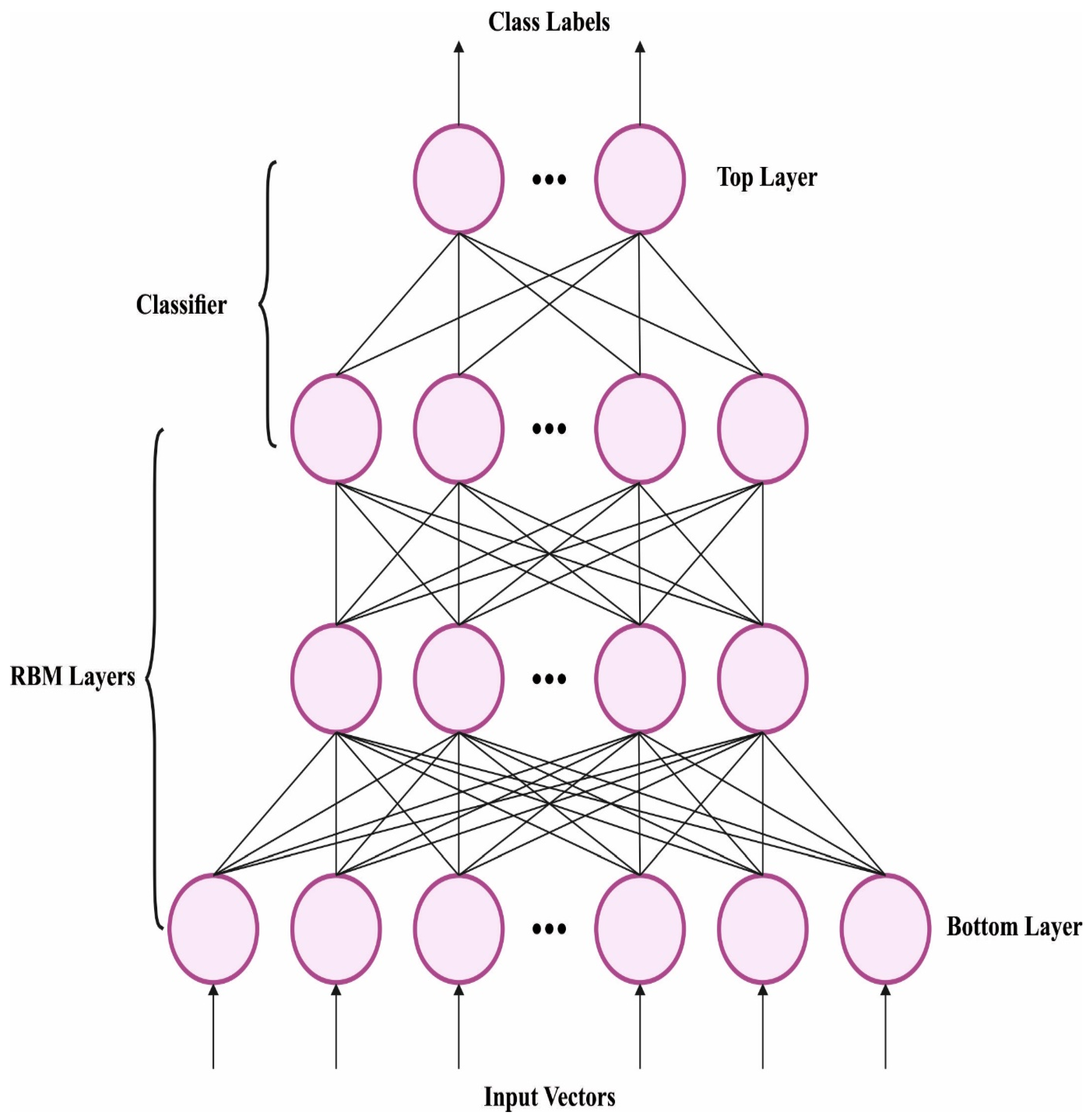
In this study, the DBN model is exploited for land cover classification. Deep Belief Network (DBN) is a probabilistic generalization mechanism that has multiple hidden layers [21]. Through updating the weights amongst neurons and training the network, the whole network is capable of recovering input dataset by the maximum probability. The DBN is made up of two networks. A number of Restricted Boltzmann machine (RBMs) are superimposed at the bottom of the network, and the RBM of every layer alter the variable θ, such that the feature of the sampling data is transmitted to the hidden layer through the maximum probability, and later the extracted feature values are considered as an input of the succeeding RBM. The data are extracted layer-wise through several RBMs, and lastly, higher-level data feature values are attained. Along with the DBN is a BPNN entity classifier. Now, a label set is attached to the topmost layer. Simultaneously, the high-level eigenvalue extracted by several RBMs is considered the input of BPNN for supervised learning. Now, the network adjusts the parameter value between different networks based on the BP and, lastly, constructs the DBN. Figure 2 showcases the framework of DBN.

DBN is composed of stacked RBM that is learned layer-wise via unsupervised greedy method. Assume the initial weight, train the initial RBM and utilize the output as an input to following layer. The output of lowermost RBM is frequently applied as an input of uppermost RBM. In this circumstance, assume that the neuron of the hidden layer h and visible layer v of RBM use binary numbers within [0, 1]. Assume (v, h), the energy function can be determined:

$$E\left(v,h|\theta \right)=-{\displaystyle \sum }_{i=1}^m{\displaystyle \sum }_{j=1}^n{\nu }_i{\omega }_{ij}{h}_j-{\displaystyle \sum }_{i=1}^m{a}_i{\nu }_i-{\displaystyle \sum }_{j=1}^n{b}_j{h}_j$$

(7)

From the expression, a_j and b_j denotes the deviation parameter of the i-th visible unit and jth hidden unit correspondingly, where m, n represents the maximum possible range of visible and hidden layers; ω_ij indicates the connection weight; {a_j, ω_ij, b_j} shows the parameters θ of RBM.

$$P\left(v,h|\theta \right)=\frac{1}{Z_{\theta }}-e^{-E\left(v,h|\theta \right)}$$

(8)

$$Z_{\theta }={\displaystyle \sum }_v{\displaystyle \sum }_h{e}^{-E(v,h|\theta )}$$

(9)

Now $Z_{\theta }$ represent the regularization factor.

RBM has two-layer NN such as h and v hidden and visual layers. The unsupervised learning capability of RBM has gained popularity; Hinton 2002 introduced contrast divergence (CD) algorithm, a fast-learning mechanism for RBM. The conditional probability is based on the principles of Bayesian formula:

$$p\left(h_j=1|v\right)=\sigma \left(b_j+{\displaystyle \sum }_i{\omega }_{ij}{v}_i\right)$$

(10)

$$p\left(v_i=1|h\right)=\sigma \left(a_i+{\displaystyle \sum }_i{\omega }_{ij}{h}_j\right)$$

(11)

where σ(x) shows the logistic function.

$$\mathsf{\sigma }\left(\mathrm{x}\right)=\frac{1}{1+{\mathrm{e}}^{-\mathrm{x}}}$$

(12)

Hinton introduced CD algorithm to calculate the updated formula of every parameter. Especially initialization of the visible layer based on the initial input sample; then, evaluate the equation of conditional probability and the conditional probability of hidden neurons based on value of visible layer; last, Gibbs sampling is utilized for extracting a sample by the computed probability.

$$W_{ij}=E(⟨V_i{h}_j⟩{}_{data}-⟨V_i{h}_j⟩{}_{recon})$$

(13)

$$a_i=E(⟨V_i⟩{}_{data}-⟨V_i⟩{}_{recon})$$

(14)

$$b_j=E(⟨h_j⟩{}_{data}-⟨h_j⟩{}_{recon})$$

(15)

Now, ε represents the learning rate, ⟨∙⟩_data and ⟨∙⟩_recon is the mathematical expectation of the data itself and after model reconstruction, correspondingly. With that condition, appropriate weight was attained, and the same technique was used until the entire weight of RBM was rehabilitated.

2.3. Hyper Parameter Tuning Using Truncate Swarm Algorithm (TSA)

Finally, the TSA is used for optimal hyper parameter tuning of the DBN model. Ref. [22] proposed a TSA based on the social behaviors of tunicate looking for prey. During hunting, marine invertebrate makes use of water jet and swarm intelligence to find prey. Every tunicate might rapidly discharge formerly inhaled seawater via the siphons of atrium, which generate a type of jet propulsion that propels it quickly. Furthermore, tunicate displays SI while they share searching information regarding the food position. The tunicate was needed to meet the subsequent 3 essential constraints to establish the mathematical modeling of jet propulsion model:

• Avoid clashes between every searching agent.
• Every agent is assured of moving towards the optimum individual.
• Make the searching agent converges to the area nearby the optimum individual.

2.3.1. Elude Clashes between Every Searching Agent

The subsequent formula is used to evaluate the new position of the agent to prevent searching agent from generating unwanted clashes:

$$\stackrel{\rightharpoonup }{A}=\frac{\stackrel{\rightharpoonup }{G}}{\stackrel{\rightharpoonup }{M}}$$

(16)

$$\stackrel{\rightharpoonup }{G}=c_2+c_3-\stackrel{\rightharpoonup }{F}$$

(17)

$$\stackrel{\rightharpoonup }{F}=2\cdot c_1$$

(18)

where $\stackrel{\rightharpoonup }{A}$ represents a vector used to search for the novel location of every agent; $\stackrel{\rightharpoonup }{G}$ represent gravity; $\stackrel{\rightharpoonup }{F}$ shows the water flow in the deep sea; $c_1,$ $c_2$, and $c_3$ denotes three randomly generated numbers within [0, 1]. $M$ indicates a vector the value where it is formulated by the social strength betwixt the searching agent and is determined by:

$$\stackrel{\rightharpoonup }{M}=P_{min}+c_1\cdot \left(P_{max}-P_{min}\right)$$

(19)

where the incipient and secondary speed enables searching agent to form social interaction can be represented as $P_{min}$ and $P_{max}$ are set to 1 and 4, correspondingly.

2.3.2. Pathfinding to the Optimal Individual

After solving clashes between nearby searching agents, the agents must move toward the nearby individual having the maximum fitness values. The mathematical modeling of moving to the better searching agent can be formulated by:

$$\stackrel{\rightharpoonup }{PD}=\left|\stackrel{\rightharpoonup }{X_{best}}-r_{rand}\cdot \stackrel{\rightharpoonup }{X\left(t\right)}\right|$$

(20)

This is Equation (20), $\stackrel{\rightharpoonup }{PD}$ represent the vector that characterizes the spatial distance between the tunicate and the target food; $\stackrel{\rightharpoonup }{X_{best}}$ refers to food that is at the location of the existing optimum individual; $r_{rand}$ indicates a random integer within $\left[0,1\right]$ and $\stackrel{\rightharpoonup }{X\left(t\right)}$ store the position data of the existing searching agent from the t-th iteration.

2.3.3. Make the Searching Agent Converge to the Optimal Individual

In order to make the searching agent perform adequate local exploration nearby the optimum individual to search for the optimum solution of the existing iteration [23], their positions are evaluated by Equation (21):

$$X\left(t\right)=\{\begin{array}{l}{X}_{besi}-\stackrel{\rightharpoonup }{A}\cdot \stackrel{\rightharpoonup }{PD},if{r}_{rand}<0.5\hfill \\ \hfill \\ X_{besi}+\stackrel{\rightharpoonup }{A}\cdot \stackrel{\rightharpoonup }{PD},if{r}_{rand}\ge 0.5\hfill \end{array}$$

(21)

At ‘t’ iteration, every searching agent explores the area nearby the optimum individual X_best and assign the outcome to X(t) for updating its location.

2.3.4. Swarm Behavior

The swarming behaviors of tunicate transmit position data betwixt the searching agents. This can be performed through the optimum individual and the location upgraded by prior individual based on swarming performance, and it can be mathematically modeled in the following:

$$X_i\left(\stackrel{\rightharpoonup }{t}+1\right)=\to \{\begin{array}{ll}\frac{\stackrel{\rightharpoonup }{X_i}\left(t\right)+X_{i-1}\left(\stackrel{\rightharpoonup }{t}+1\right)}{\to 2+c_1}\to \to \hfill & if i>1\hfill \\ \stackrel{\rightharpoonup }{X_i}\left(t\right)\hfill & if i=1\hfill \end{array}$$

(22)

whereas $i=1,\dots ,N,$ $N$ refers to the size of tunicate population, $X_i\left(\stackrel{\rightharpoonup }{t}+1\right)$ indicates the location of present searching agent, $X_{i-1}\left(\stackrel{\rightharpoonup }{t}+1\right)$ denotes the location of the preceding searching agent, and $X_i\left(\stackrel{\rightharpoonup }{t}\right)$ is evaluated using Equation (21). To demonstrate the step-by-step process of TSA, the major step to upgrade the position of searching agent is as follows:

• Step 1: Initialize the original population of searching agent $X.$
• Step 2: Assign value to $\max$-iteration and other initial variables.
• Step 3: Calculate the fitness values of every tunicate and choose the individual with the better fitness values as the optimum searching agent.
• Step 4: Upgrade the position of every searching agent using Equation (22).
• Step 5: Keep every search agent in the search space.
• Step 6: Evaluate the fitness values of every upgrade searching agent; if there is the best individual than the preceding optimum searching agent in the population, upgrade $X_{besi}.$
• Step 7: If the maximal iteration is attained, then the procedure stops. Or else, continue with steps 4–7.
• Step 8: Output the better individual $\left(X_{besi}\right)$.

Selective fitness is a vital factor in the TSA system. The solution encoder was used for measuring the aptitude (goodness) of candidate results. At this point, the accuracy value is the important state employed to design a fitness function.

$$Fitness=\max \left(P\right)$$

(23)

$$P=\frac{TP}{TP+FP}$$

(24)

From the expression, TP represents the true positive, and FP denotes the false positive value.

3. Data and Data Processing

3.1. Study Area

Nallamalla Forest is the largest stretch of undisturbed forest in South India. It is found on Nallamalla hills which are part of Eastern Ghats and spread over Kadapa, Kurnool, Guntur, Prakasam, and Mahabubnagar districts. The largest part of the forest is Nagarjunsagar-Srisailam Tiger Reserve which has a feasible tiger population. Leopard sightings are more common. Between the streams Krishna and Pennar, they follow a near north-south alignment that roughly corresponds to the Coromandel Coast for a distance of about 430 km. Its northern bounds are defined by the Palnadu bowl’s plain terrain, while its southern boundary is formed by the Tirupati slopes. Its coordinates are 16.0131 North and 78.9717 East. The slopes are an older structure that has generally persisted and crumbled over time. The modern standard increase is about 520 m, reaching 1100 m at Bhairani Konda and 1048 m at Gundla Brahmeswara. The town of Cumbum is located northwest of each of these pinnacles. Moreover, there are a variety of summits above 800 m. Typically, the forests have huge expanses of greenery, grass, and mountains.

3.2. Satellite Images

Images from the LANDSAT 7(ETM+) satellite were utilized to analyze the LULC. On 15 April 1999, NASA launched LANDSAT 7, which is equipped with the ETM+ (Enhanced Thematic Mapper plus) with four modes: SWIR (Shortwave Infrared), TIR (Thermal infrared—Thermal infrared range), PAN (Panchromatic—Panchromatic range), and VNIR (Visible and Near Infrared). The Thermal spectral bands are provided by the LANDSAT 7 ETM+ instruments, which offer an improvement from 120 m to 60 m. From GloVis, EarthExplorer, and LandsatLook Viewer, users can access the LANDSAT 7 ETM+ scenes.

The research study has been conducted by LANDSAT 7 images from [https://www.usgs.gov/landsat-missions/landsat-data-access]. On every occasion the image is oriented North Up, there is an overall of 11 bands or projection units in meters. Band 4 provides vegetation-related geographical features in TIFF format. The scenes that are pulled are TIFF files that are RASTER pictures of Bands 1, 2, 3, 4, 5, and 7. Multiple pages and layers, as well as red, blue, and green, are supported by the scenes. Multiple layer images with a depth of either 8 bits per channel or 16 bits per channel can be found in a single TIFF file. LANDSAT 7 scenes were taken from the time period of 2014 to 2022 for the analysis of the LULC over the years.

4. Results and Discussion

In this section, the performance of the TSADL-LULCCD model is tested using the data collected from Nallamalla forest, India. The details related to the target region used for simulation analysis are shown in

Table 1. Details on Database.

Class	Area (km2)	Size	% of Area
Grassland	321.30	321.00	30.20
Agriculture	182.90	183.00	17.19
Barren land	231.90	232.00	21.80
Water	327.70	328.00	30.80
Total	1063.80	1064.00	100.00

. Figure 3 illustrates the sample images.

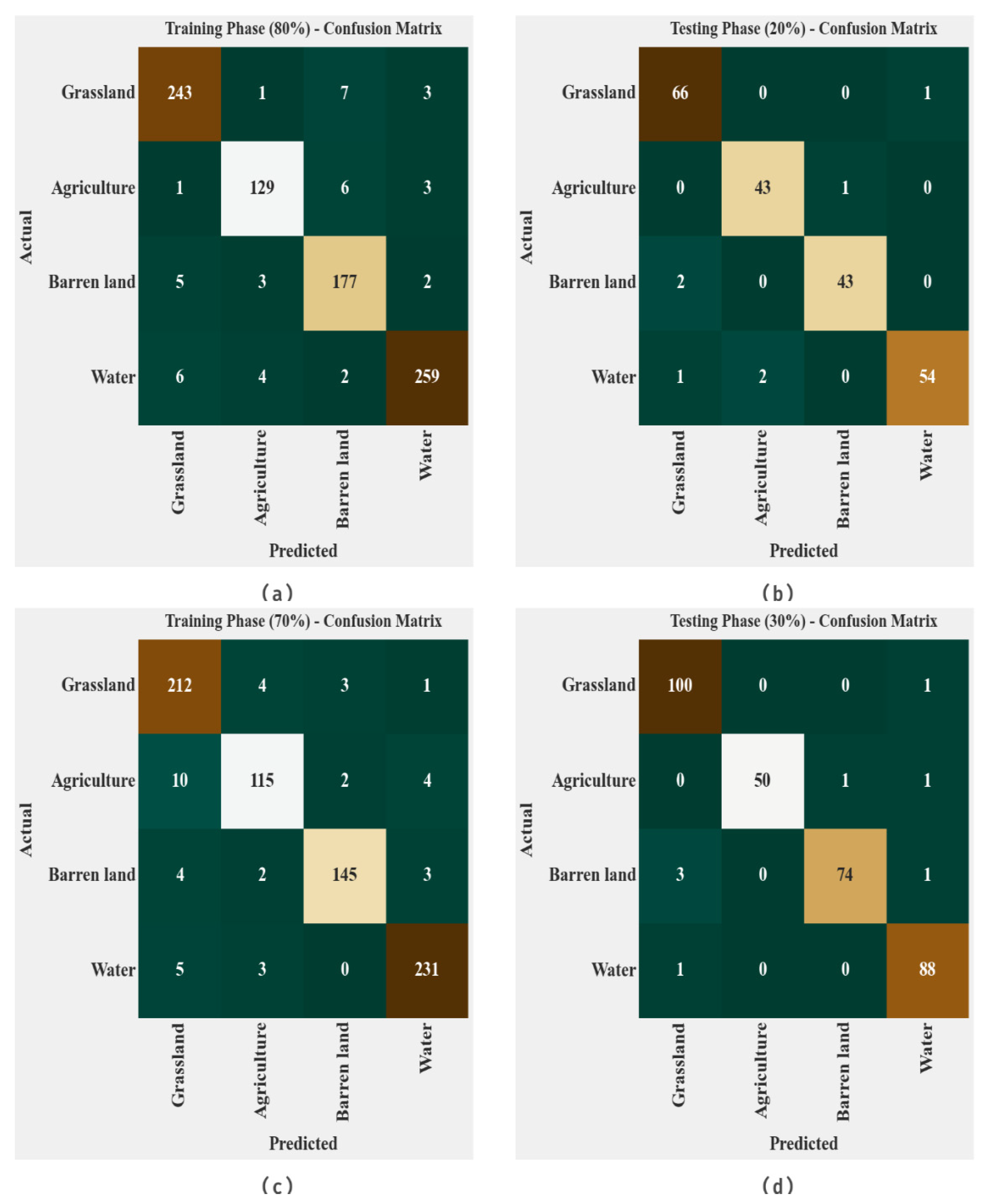
The confusion matrices of the TSADL-LULCCD model are clearly demonstrated in Figure 4. On 80% of the TR database, the TSADL-LULCCD method has recognized 243 samples in grassland, 129 samples in agriculture, 177 samples in barren land, and 259 samples in water. Simultaneously on 20% of the TS database, the TSADL-LULCCD technique has recognized 66 samples in grassland, 43 samples in agriculture, 43 samples in barren land, and 54 samples in water. Concurrently on 70% of the TR database, the TSADL-LULCCD method has recognized 212 samples in grassland, 115 samples in agriculture, 145 samples in barren land, and 231 samples in water. Finally, on 20% of the TS database, the TSADL-LULCCD approach has recognized 100 samples in grassland, 50 samples in agriculture, 74 samples in barren land, and 88 samples in water.

In

Table 2. Classification outcome of TSADL-LULCCD approach on 80:20 of TR/TS databases.

Class	$\mathit{A}\mathit{c}\mathit{c}{\mathit{u}}_{\mathit{y}}$	$\mathit{P}\mathit{r}\mathit{e}{\mathit{c}}_{\mathit{n}}$	$\mathit{R}\mathit{e}\mathit{c}{\mathit{a}}_{\mathit{l}}$	${\mathit{F}}_{\mathit{s}\mathit{c}\mathit{o}\mathit{r}\mathit{e}}$	AUC Score	MCC
Training Phase
Grassland	97.30	95.29	95.67	95.48	96.83	93.55
Agriculture	97.88	94.16	92.81	93.48	95.84	92.22
Barren land	97.06	92.19	94.65	93.40	96.20	91.53
Water	97.65	97.00	95.57	96.28	97.10	94.57
Average	97.47	94.66	94.67	94.66	96.49	92.97
Testing Phase
Grassland	98.12	95.65	98.51	97.06	98.23	95.70
Agriculture	98.59	95.56	97.73	96.63	98.27	95.75
Barren land	98.59	97.73	95.56	96.63	97.48	95.75
Water	98.12	98.18	94.74	96.43	97.05	95.18
Average	98.36	96.78	96.63	96.69	97.76	95.60

and Figure 5, the overall classification outcomes of the TSADL-LULCCD model with 80:20 of the TR/TS database are provided. On the TR database, the TSADL-LULCCD model has recognized grassland samples with $acc{u}_y$ of 97.30%, $pre{c}_n$ of 95.29%, $rec{a}_l$ of 95.67%, $F_{score}$ of 95.48%, $AU{C}_{score}$ of 96.83%, and MCC of 93.55%. Meanwhile, the TSADL-LULCCD model has identified agriculture samples with $acc{u}_y$ of 97.88%, $pre{c}_n$ of 94.16%, $rec{a}_l$ of 92.81%, $F_{score}$ of 93.48%, $AU{C}_{score}$ of 95.84%, and MCC of 92.22%. Furthermore, the TSADL-LULCCD model has categorized barren land samples with $acc{u}_y$ of 97.06%, $pre{c}_n$ of 92.19%, $rec{a}_l$ of 94.65%, $F_{score}$ of 93.40%, $AU{C}_{score}$ of 96.20%, and MCC of 91.53%.

On the TR database, the TSADL-LULCCD technique has recognized grassland samples with $acc{u}_y$ of 98.12%, $pre{c}_n$ of 95.65%, $rec{a}_l$ of 98.51%, $F_{score}$ of 97.06%, $AU{C}_{score}$ of 98.23%, and MCC of 95.70%. In the meantime, the TSADL-LULCCD approach has identified agriculture samples with $acc{u}_y$ of 98.59%, $pre{c}_n$ of 95.56%, $rec{a}_l$ of 97.73%, $F_{score}$ of 96.63%, $AU{C}_{score}$ of 98.27%, and MCC of 95.75%. Furthermore, the TSADL-LULCCD method has categorized barren land samples with $acc{u}_y$ of 98.59%, $pre{c}_n$ of 97.73%, $rec{a}_l$ of 95.56%, $F_{score}$ of 96.63%, $AU{C}_{score}$ of 97.48%, and MCC of 95.75%.

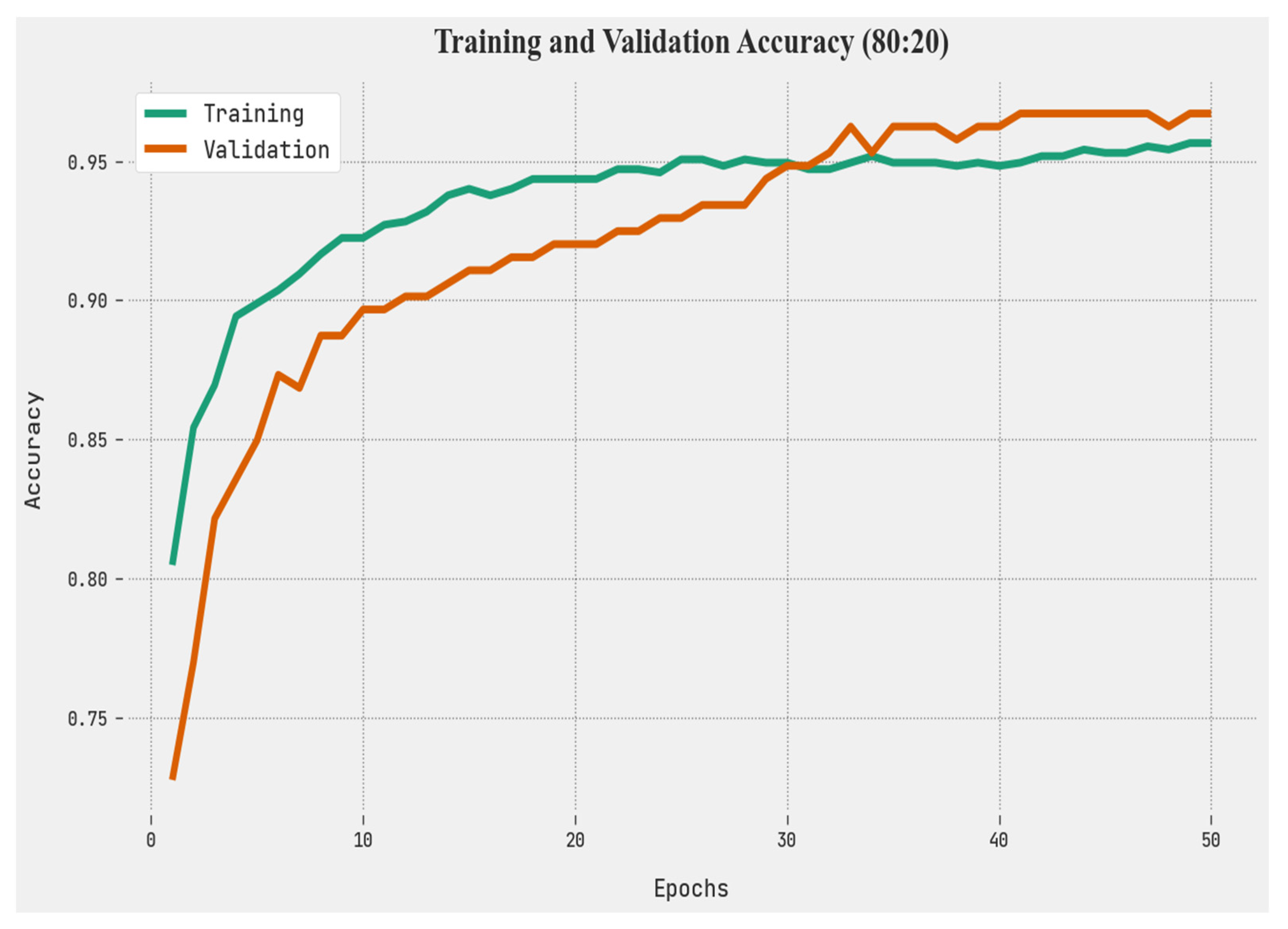
The TACC and VACC of the TSADL-LULCCD approach are inspected on 80:20 of TR/TS databases in Figure 6. The outcomes implied that the TSADL-LULCCD methodology had shown improved performance with increased values of TACC and VACC. Notably, the TSADL-LULCCD method has reached maximum TACC outcomes.

The TLS and VLS of the TSADL-LULCCD approach are tested on 80:20 of TR/TS databases in Figure 7. The figure exhibited shows that the TSADL-LULCCD method has revealed better performance with the least values of TLS and VLS. Seemingly, the TSADL-LULCCD algorithm has resulted in reduced VLS outcomes.

A clear precision-recall investigation of the TSADL-LULCCD approach on 80:20 TR/TS databases is seen in Figure 8. The results show the TSADL-LULCCD method has enhanced values of precision-recall values.

The detailed ROC study of the TSADL-LULCCD technique on 80:20 TR/TS databases is shown in Figure 9. The outcomes denoted the TSADL-LULCCD algorithm has shown its ability to categorize different classes under a test database.

In

Table 3. Classification outcome of TSADL-LULCCD approach on 70:30 of TR/TS databases.

Training/Testing (70:30)
Classes	$\mathit{A}\mathit{c}\mathit{c}{\mathit{u}}_{\mathit{y}}$	$\mathit{P}\mathit{r}\mathit{e}{\mathit{c}}_{\mathit{n}}$	$\mathit{R}\mathit{e}\mathit{c}{\mathit{a}}_{\mathit{l}}$	${\mathit{F}}_{\mathit{s}\mathit{c}\mathit{o}\mathit{r}\mathit{e}}$	AUC Score	MCC
Training Phase
Grassland	96.37	91.77	96.36	94.01	96.37	91.47
Agriculture	96.64	92.74	87.79	90.20	93.16	88.22
Barren land	98.12	96.67	94.16	95.39	96.65	94.23
Water	97.85	96.65	96.65	96.65	97.53	95.07
Average	97.24	94.46	93.74	94.06	95.93	92.25
Testing Phase
Grassland	98.44	96.15	99.01	97.56	98.59	96.43
Agriculture	99.38	100.00	96.15	98.04	98.08	97.69
Barren land	98.44	98.67	94.87	96.73	97.23	95.74
Water	98.75	96.70	98.88	97.78	98.79	96.92
Average	98.75	97.88	97.23	97.53	98.17	96.70

and Figure 10, the overall classification outcomes of the TSADL-LULCCD method with 70:30 of the TR/TS database are provided. On the TR database, the TSADL-LULCCD approach has recognized grassland samples with $acc{u}_y$ of 96.37%, $pre{c}_n$ of 91.77%, $rec{a}_l$ of 96.36%, $F_{score}$ of 94.01%, $AU{C}_{score}$ of 96.37%, and MCC of 91.47%. In the meantime, the TSADL-LULCCD method has identified agriculture samples with $acc{u}_y$ of 96.64%, $pre{c}_n$ of 92.74%, $rec{a}_l$ of 87.79%, $F_{score}$ of 90.20%, $AU{C}_{score}$ of 93.16%, and MCC of 88.22%. Additionally, the TSADL-LULCCD model has categorized barren land samples with $acc{u}_y$ of 98.12%, $pre{c}_n$ of 96.67%, $rec{a}_l$ of 94.16%, $F_{score}$ of 95.39%, $AU{C}_{score}$ of 96.65%, and MCC of 94.23%.

On the TR database, the TSADL-LULCCD method has recognized grassland samples with $acc{u}_y$ of 98.44%, $pre{c}_n$ of 96.15%, $rec{a}_l$ of 99.01%, $F_{score}$ of 97.56%, $AU{C}_{score}$ of 98.59%, and MCC of 96.43%. In the meantime, the TSADL-LULCCD approach has identified agriculture samples with $acc{u}_y$ of 99.38%, $pre{c}_n$ of 100.00%, $rec{a}_l$ of 96.15%, $F_{score}$ of 98.04%, $AU{C}_{score}$ of 98.08%, and MCC of 97.69%. Additionally, the TSADL-LULCCD technique has categorized barren land samples with $acc{u}_y$ of 98.44%, $pre{c}_n$ of 98.67%, $rec{a}_l$ of 94.87%, $F_{score}$ of 96.73%, $AU{C}_{score}$ of 97.23%, and MCC of 95.74%.

The TACC and VACC of the TSADL-LULCCD approach are investigated on 70:30 of TR/TS databases in Figure 11. The figure shows the TSADL-LULCCD technique has shown improved performance with increased values of TACC and VACC. Notably, the TSADL-LULCCD approach has achieved maximum TACC outcomes.

The TLS and VLS of the TSADL-LULCCD technique are tested on 70:30 of TR/TS databases in Figure 12. The figure designated the TSADL-LULCCD method has revealed better performance with the least values of TLS and VLS. Seemingly, the TSADL-LULCCD approach has reduced VLS outcomes.

A clear precision-recall inspection of the TSADL-LULCCD method on 70:30 TR/TS databases is seen in Figure 13. The outcomes show the TSADL-LULCCD approach has enhanced values of precision-recall values.

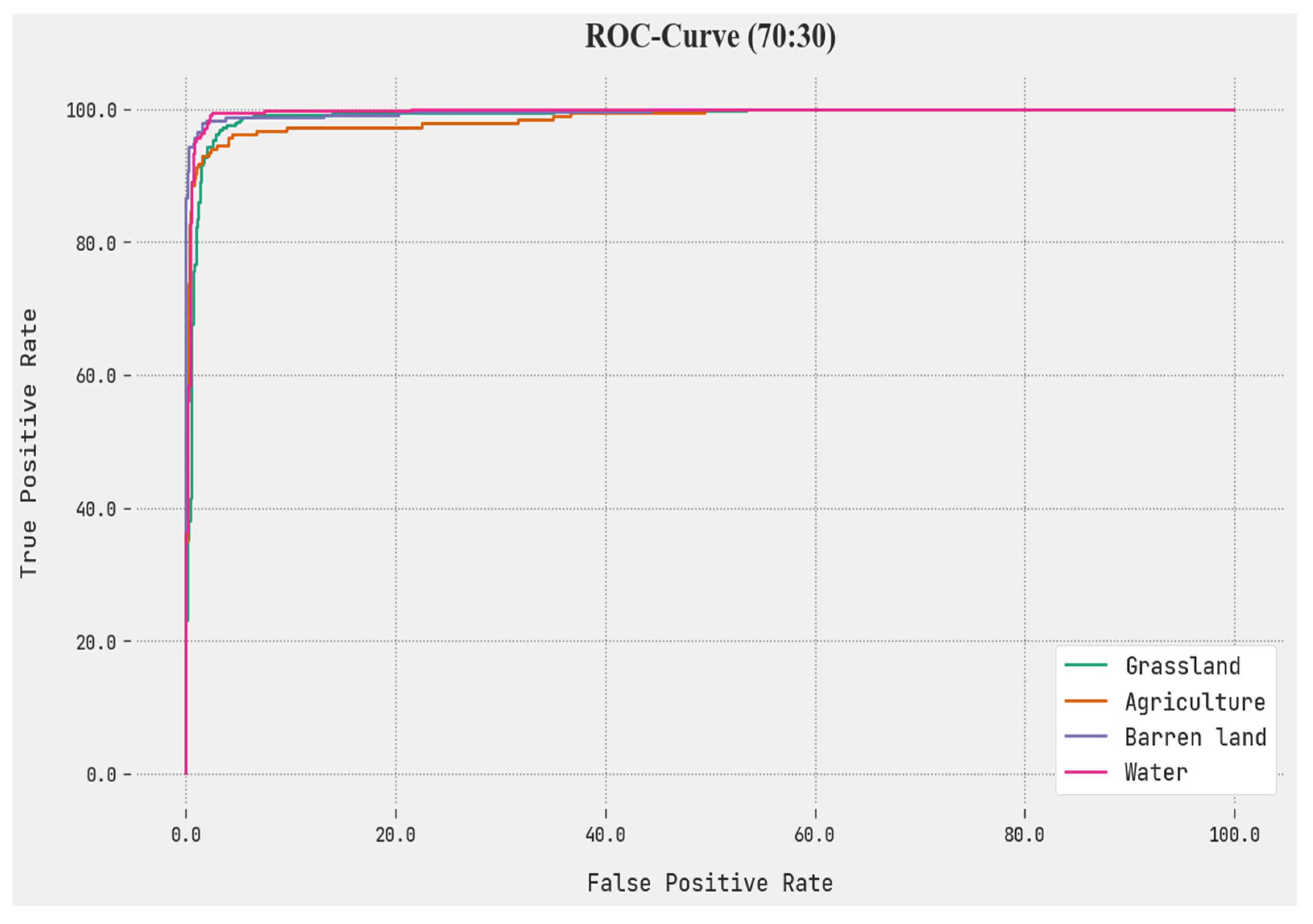
Next, a detailed ROC study of the TSADL-LULCCD method on 70:30 TR/TS databases is shown in Figure 14. The outcomes exhibit the TSADL-LULCCD technique has shown its ability to classify different classes.

Finally, an extended comparative study of the TSADL-LULCCD model with recent models is given in

Table 4. Time Comparison between KNN, LSH with TRT, LSH without TRT Models.

Algorithm	Average CPU Utilization (%)	Average GPU Utilization (%)	Time Taken (in ms)
TSADL-LULCCD	71.3	21.1	353.176
Stochastic Gradient Descent (SGD)	27.3	50.6	150.577
Symbolic ML via Genetic Algorithms (GA)	33.5	40.7	268.784

[24]. Figure 15 represents $acc{u}_y$ examination of the TSADL-LULCCD model with recent models. The results signified that the DT and LR models had reported worse outcomes with minimum $acc{u}_y$ of 91.18% and 92.03%, respectively. Followed by the SGD and ExGBT models, which have certainly accomplished closer $acc{u}_y$ of 93.11% and 93.13%, respectively. Meanwhile, the GA and DL models have revealed reasonable outcomes with $acc{u}_y$ of 95.24% and 97.88%, respectively. However, the TSADL-LULCCD model has exhibited its improved performance with $acc{u}_y$ of 98.75%.

Evaluation of our TSADL with LULCCD gives against SGD and GA algorithms insights to learn the time taken to analyze the characteristics of satellite images and to classify the nature of lands (

Table 5. Comparative analysis of TSADL-LULCCD approach with other approaches.

Methods	$\mathit{A}\mathit{c}\mathit{c}{\mathit{u}}_{\mathit{y}}$	$\mathit{P}\mathit{r}\mathit{e}{\mathit{c}}_{\mathit{n}}$	$\mathit{R}\mathit{e}\mathit{c}{\mathit{a}}_{\mathit{l}}$	${\mathit{F}}_{\mathit{s}\mathit{c}\mathit{o}\mathit{r}\mathit{e}}$
TSADL-LULCCD	98.75	97.88	97.23	97.53
Decision Tree (DT)	91.18	91.92	93.56	91.82
Logistic Regression (LR)	92.03	93.41	93.66	94.95
Stochastic Gradient Descent (SGD)	93.11	94.06	93.10	95.08
Extreme Gradient Boosted Trees (ExGBT)	93.13	96.42	93.75	95.98
Symbolic ML via Genetic Algorithms (GA)	95.24	95.75	95.79	95.88
Deep Learning (DL)	97.88	96.51	95.94	96.30

,

Table 6. Training and Validation process results.

Algorithm	Epoch	Iterations	RMSE	Log-Loss (%)	Validation Loss
TSADL-LULCCD	10	150	87.86	31.51	0.30
	20	300	66.76	29.88	0.32
	30	450	45.84	28.69	0.34
Stochastic Gradient Descent (SGD)	10	150	88.17	31.59	0.49
	20	300	67.51	29.96	0.47
	30	450	48.04	28.77	0.46
Symbolic ML via Genetic Algorithms (GA)	10	150	89.33	31.44	0.52
	20	300	67.93	29.80	0.53
	30	450	46.56	28.62	0.65

).

Figure 16 signifies $pre{c}_n$ inspection of the TSADL-LULCCD method with recent approaches. The results signified that the DT and LR methods had reported worse outcomes with minimum $pre{c}_n$ of 91.92% and 93.41%, correspondingly. Then, the SGD and GA models have exhibited certainly closer $pre{c}_n$ of 94.06% and 95.75% correspondingly. In the meantime, the ExGBT and DL models have revealed reasonable outcomes with $pre{c}_n$ of 96.42% and 96.51%, respectively. However, the TSADL-LULCCD method has exhibited its improved performance with $pre{c}_n$ of 97.88%.

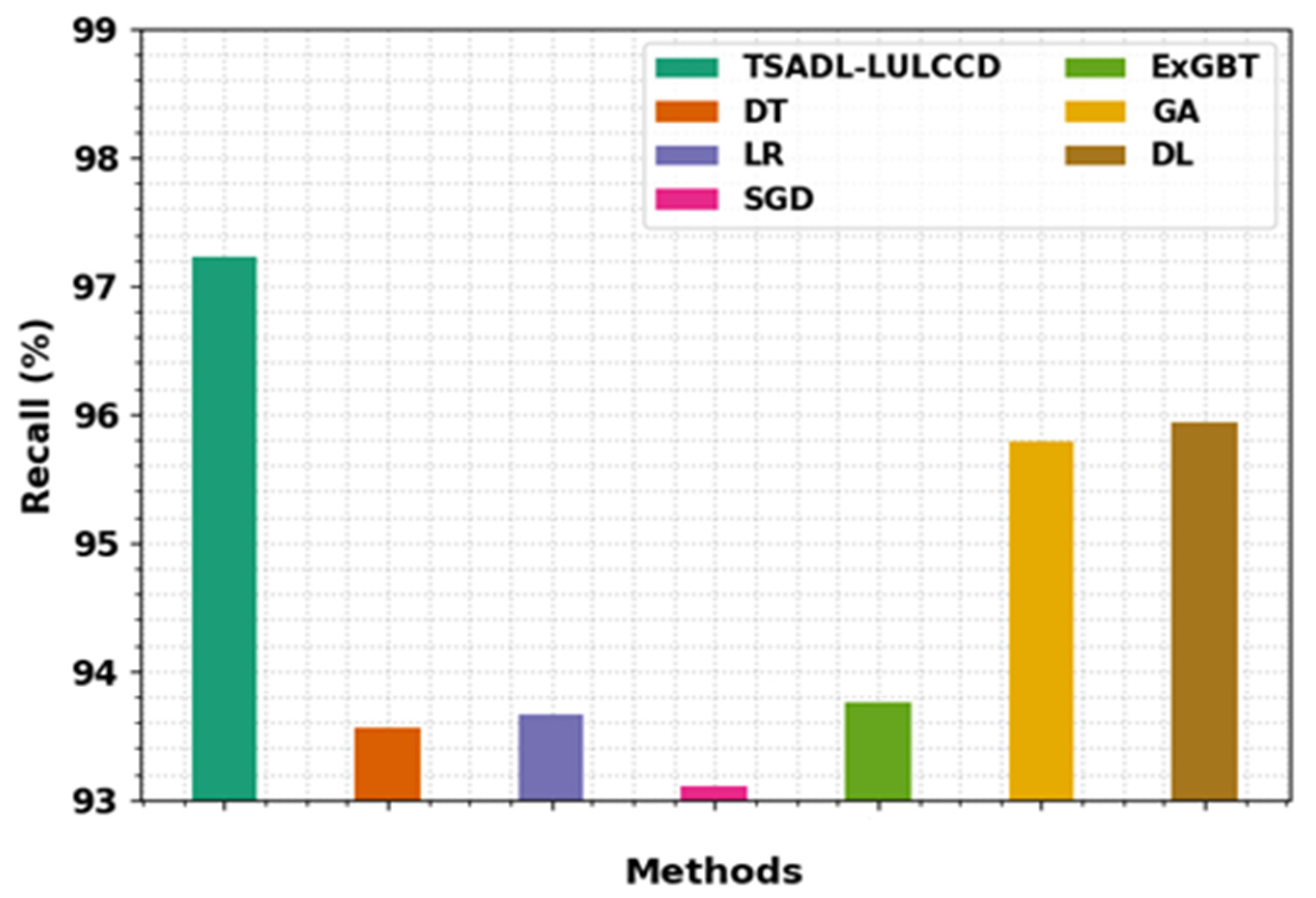
Figure 17 represents $rec{a}_l$ inspection of the TSADL-LULCCD model with recent models. The results signified that the SGD and DT approaches had reported worse outcomes with minimum $rec{a}_l$ of 93.1% and 93.56%, respectively. Followed by the LR and ExGBT models, which have accomplished certainly closer $rec{a}_l$ of 93.66% and 93.75%, respectively. In the meantime, the GA and DL models have revealed reasonable outcomes with $rec{a}_l$ of 95.79% and 95.94% correspondingly. However, the TSADL-LULCCD method has shown its improved performance with $rec{a}_l$ of 97.23%.

Figure 18 denotes $F_{score}$ investigation of the TSADL-LULCCD model with recent methods. The results signified that the DT and LR approaches had reported worse outcomes with minimum $F_{score}$ of 91.82% and 94.95%, correspondingly. Followed by the SGD and ExGBT models, which have certainly accomplished closer $F_{score}$ of 95.08% and 95.88% correspondingly. Meanwhile, the GA and DL methods have revealed reasonable outcomes with $F_{score}$ of 95.98% and 96.3%, correspondingly. However, the TSADL-LULCCD method has exhibited improved performance with $F_{score}$ of 97.53%. These results assured the better performance of the TSADL-LULCCD model compared to recent approaches.

5. Conclusions

Remote sensing (RS) is a very reliable and efficient method for monitoring environmental and terrain changes. Topographic maps are crucial to science, research, planning, and administration in the modern world. It is entirely feasible to discern changes based on RS data collected at two distinct periods. In this article, we have developed a new TSADL-LULCCD technique for land cover classification in Nallamalla Forest, India. The presented TSADL-LULCCD technique mainly focuses on the identification and classification of land use in the Nallamalla forest using LANDSAT 7 images. Primarily, the presented TSADL-LULCCD technique employed an Adam optimizer with a dense EfficientNet model for feature extraction. For land cover classification, the TSADL-LULCCD technique exploited the TSA with the DBN model. The experimental validation of the TSADL-LULCCD technique is tested on LANDSAT-7-based Nallamalla region images. The experimental results stated that the TSADL-LULCCD technique exhibits better performance over other existing models in terms of different evaluation measures. In the future, we are planning to include forest classification with the help of hybrid DL fusion techniques that can be employed to improve classification performance.

References

1. Talukdar, S.; Singha, P.; Mahato, S.; Pal, S.; Liou, Y.A.; Rahman, A. Land-use land-cover classification by machine learning classifiers for satellite observations—A review. Remote Sens. 2020, 12, 1135. [Google Scholar] [CrossRef] [Green Version]
2. Xu, Y.; Du, B.; Zhang, L.; Cerra, D.; Pato, M.; Carmona, E.; Prasad, S.; Yokoya, N.; Hänsch, R.; Le Saux, B. Advanced multi-sensor optical remote sensing for urban land use and land cover classification: Outcome of the 2018 IEEE GRSS data fusion contest. IEEE J. Sel. Top. Appl. Earth Obs. Remote Sens. 2019, 12, 1709–1724. [Google Scholar] [CrossRef]
3. Lenco, D.; Interdonato, R.; Gaetano, R.; Minh, D.H.T. Combining Sentinel-1 and Sentinel-2 Satellite Image Time Series for land cover mapping via a multi-source deep learning architecture. ISPRS J. Photogramm. Remote Sens. 2019, 158, 11–22. [Google Scholar]
4. Thepade, S.D.; Dindorkar, M.R. Fusing deep convolutional neural network features with Thepade’s SBTC for land usage identification. Eng. Sci. Technol. Int. J. 2022, 27, 101014. [Google Scholar] [CrossRef]
5. Wong, Y.; Lee, H.Y.; Chen, Y.C.; Zeng, Y.T.; Chern, Y.R.; Chen, N.T.; Lung, S.C.C.; Su, H.J.; Wu, C.D. Using a land use regression model with machine learning to estimate ground level PM 2.5. Environ. Pollut. 2021, 277, 116846. [Google Scholar] [CrossRef]
6. Helber, P.; Bischke, B.; Dengel, A.; Borth, D. Eurosat: A novel dataset and deep learning benchmark for land use and land cover classification. IEEE J. Sel. Top. Appl. Earth Obs. Remote Sens. 2019, 12, 2217–2226. [Google Scholar] [CrossRef] [Green Version]
7. Pan, X.; Wang, Z.; Gao, Y.; Dang, X.; Han, Y. Detailed and automated classification of land use/land cover using machine learning algorithms in Google Earth Engine. Geocarto Int. 2022, 37, 5415–5432. [Google Scholar] [CrossRef]
8. Tian, F.; Wu, B.; Zeng, H.; Watmough, G.R.; Zhang, M.; Li, Y. Detecting the linkage between arable land use and poverty using machine learning methods at global perspective. Geogr. Sustain. 2022, 3, 7–20. [Google Scholar] [CrossRef]
9. Yoo, S.; Lee, J.; Farkoushi, M.G.; Lee, E.; Sohn, H.G. Automatic generation of land use maps using aerial orthoimages and building floor data with a Conv-Depth Block (CDB) ResU-Net architecture. Int. J. Appl. Earth Obs. Geoinf. 2022, 107, 102678. [Google Scholar] [CrossRef]
10. Masolele, R.N.; De Sy, V.; Herold, M.; Marcos, D.; Verbesselt, J.; Gieseke, F.; Mullissa, A.G.; Martius, C. Spatial and temporal deep learning methods for deriving land-use following deforestation: A pan-tropical case study using Landsat time series. Remote Sens. Environ. 2021, 264, 112600. [Google Scholar] [CrossRef]
11. Yao, Y.; Yan, X.; Luo, P.; Liang, Y.; Ren, S.; Hu, Y.; Han, J.; Guan, Q. Classifying land-use patterns by integrating time-series electricity data and high-spatial resolution remote sensing imagery. Int. J. Appl. Earth Obs. Geoinf. 2022, 106, 102664. [Google Scholar] [CrossRef]
12. Zhang, P.; Ke, Y.; Zhang, Z.; Wang, M.; Li, P.; Zhang, S. Urban land use and land cover classification using novel deep learning models based on high spatial resolution satellite imagery. Sensors 2018, 18, 3717. [Google Scholar] [CrossRef] [Green Version]
13. Abdi, A.M. Land cover and land use classification performance of machine learning algorithms in a boreal landscape using Sentinel-2 data. GIScience Remote Sens. 2020, 57, 1–20. [Google Scholar] [CrossRef] [Green Version]
14. Zhu, Q.; Guo, X.; Deng, W.; Guan, Q.; Zhong, Y.; Zhang, L.; Li, D. Land-use/land-cover change detection based on a Siamese global learning framework for high spatial resolution remote sensing imagery. ISPRS J. Photogramm. Remote Sens. 2022, 184, 63–78. [Google Scholar] [CrossRef]
15. Chang, S.; Wang, Z.; Mao, D.; Guan, K.; Jia, M.; Chen, C. Mapping the essential urban land use in changchun by applying random forest and multi-source geospatial data. Remote Sens. 2020, 12, 2488. [Google Scholar] [CrossRef]
16. Talukdar, S.; Singha, P.; Mahato, S.; Praveen, B.; Rahman, A. Dynamics of ecosystem services (ESs) in response to land use land cover (LU/LC) changes in the lower Gangetic plain of India. Ecol. Indic. 2020, 112, 106121. [Google Scholar] [CrossRef]
17. Zhang, C.; Sargent, I.; Pan, X.; Li, H.; Gardiner, A.; Hare, J.; Atkinson, M. An object-based convolutional neural network (OCNN) for urban land use classification. Remote Sens. Environ. 2018, 216, 57–70. [Google Scholar] [CrossRef] [Green Version]
18. Ekim, B.; Sertel, E. Deep neural network ensembles for remote sensing land cover and land use classification. Int. J. Digit. Earth 2021, 14, 1868–1881. [Google Scholar] [CrossRef]
19. Nayak, D.R.; Padhy, N.; Mallick, K.; Zymbler, M.; Kumar, S. Brain Tumor Classification Using Dense Efficient-Net. Axioms 2022, 11, 34. [Google Scholar] [CrossRef]
20. Wang, L.; Liu, Z. Data-driven product design evaluation method based on multi-stage artificial neural network. Appl. Soft Comput. 2021, 103, 107117. [Google Scholar] [CrossRef]
21. Fang, Z.; Roy, K.; Mares, J.; Sham, C.W.; Chen, B.; Lim, J.B. Deep learning-based axial capacity prediction for cold-formed steel channel sections using Deep Belief Network. Structures 2021, 33, 2792–2802. [Google Scholar] [CrossRef]
22. Kaur, S.; Awasthi, L.K.; Sangal, A.L.; Dhiman, G. Tunicate Swarm Algorithm: A new bio-inspired based metaheuristic paradigm for global optimization. Eng. Appl. Artif. Intell. 2020, 90, 103541. [Google Scholar] [CrossRef]
23. Cui, Y.; Shi, R.; Dong, J. CLTSA: A Novel Tunicate Swarm Algorithm Based on Chaotic-Lévy Flight Strategy for Solving Optimization Problems. Mathematics 2022, 10, 3405. [Google Scholar] [CrossRef]
24. Sudeesh, S.; Sudhakar Reddy, C. Forest fire monitoring in Nagarjunasagar-Srisailam Tiger Reserve, Andhra Pradesh, India using geospatial techniques. Natl. Acad. Sci. Lett. 2013, 36, 437–446. [Google Scholar] [CrossRef]
Figure 1. Workflow of TSADL-LULCCD approach.
Applsci 13 01173 g001
Figure 2. Framework of DBN.
Applsci 13 01173 g002
Figure 3. (a) Map of Nallamalla Forest [16.0131° N, 78.9717° E] (b) Site View of Nallamalla Forest.
Applsci 13 01173 g003
Figure 4. Confusion matrices of TSADL-LULCCD method (a,b) TR and TS databases of 80:20 and (c,d) TR and TS databases of 70:30.
Applsci 13 01173 g004
Figure 5. Average outcome of TSADL-LULCCD method on 80:20 of TR/TS databases.
Applsci 13 01173 g005
Figure 6. TACC and VACC analysis of TSADL-LULCCD method on 80:20 of TR/TS databases.
Applsci 13 01173 g006
Figure 7. TLS and VLS analysis of TSADL-LULCCD approach on 80:20 of TR/TS databases.
Applsci 13 01173 g007
Figure 8. Precision-recall analysis of TSADL-LULCCD approach on 80:20 of TR/TS databases.
Applsci 13 01173 g008
Figure 9. ROC analysis of TSADL-LULCCD approach on 80:20 of TR/TS databases.
Applsci 13 01173 g009
Figure 10. Average outcome of TSADL-LULCCD approach on 70:30 of TR/TS databases.
Applsci 13 01173 g010
Figure 11. TACC and VACC analysis of TSADL-LULCCD approach on 70:30 of TR/TS database.
Applsci 13 01173 g011
Figure 12. TLS and VLS analysis of TSADL-LULCCD approach on 70:30 of TR/TS databases.
Applsci 13 01173 g012
Figure 13. Precision-recall analysis of TSADL-LULCCD approach on 70:30 of TR/TS.
Applsci 13 01173 g013
Figure 14. ROC analysis of TSADL-LULCCD approach on 70:30 of TR/TS databases.
Applsci 13 01173 g014
Figure 15. A c c u y analysis of TSADL-LULCCD approach with other approaches.
Applsci 13 01173 g015
Figure 16. P r e c n analysis of TSADL-LULCCD approach with other approaches.
Applsci 13 01173 g016
Figure 17. R e c a l analysis of TSADL-LULCCD approach with other approaches.
Applsci 13 01173 g017
Figure 18. F s c o r e   analysis of TSADL-LULCCD approach with other approaches.
Applsci 13 01173 g018