Abstract
Aiming at the difficulty of fault location of multi-source transmission lines, this paper proposes a fault location method for multi-terminal transmission lines based on a fault branch judgment matrix. The fault traveling wave signal is decomposed by Complete Ensemble Empirical Mode Decomposition with Adaptive Noise (CEEMDAN), and the IMFs sensitive components that can characterize the fault characteristics of the target signals are selected by constructing a correlation-rearrangement entropy function. The arrival time of fault signals at the endpoint has been accurately calibrated by combining them with the Teager Energy Operator (TEO). To eliminate the influence of wave velocity and fault time on the location results, this paper proposes a two-terminal location method based on the line mode component to improve the location accuracy. On this basis, combined with the fault branch judgment matrix, the accurate location of multi-terminal transmission line faults is realized. This method has been shown to have high accuracy in detecting traveling wave heads, accurately judging fault branches, and producing a small error in fault location results. Compared with the existing multi-terminal transmission line fault location algorithm, it has obvious advantages and meets the needs of actual working conditions.
1. Introduction
Transmission lines, as essential carriers of electric energy transmission and long-distance transmission, are prone to faults during operation due to their use in remote areas and complex operating environments, which seriously affect the normal operation of the power grid. Therefore, accurately and quickly determining the fault location is a primary problem for transmission lines. As transmission networks continue to develop, the structure of transmission lines has become increasingly complex, and the proportion of multi-terminated transmission lines has gradually increased. The complexity of the topology of multi-terminated transmission lines is higher than traditional double-terminated transmission lines, which makes traditional fault location methods unable to meet the requirements for accurate fault location in transmission networks.
Due to its accuracy and reliability, the traveling wave method [,,] is currently one of the most effective methods for fault location of power systems. However, its applications to multi-terminal transmission lines have issues such as low reliability of positioning results, difficulty in identifying traveling wave heads, and uncertainty of traveling wave velocity [,]. Further, literature has proposed a two-terminal ranging method based on time-frequency analysis of traveling waves [,]. The fault traveling wave characteristic frequency is extracted using wavelet packets to capture the fault wave head accurately. However, this method has the problem of characteristic frequency aliasing in the case of grounding faults and has significant limitations. Parsi et al. propose a fault-locating method based on the natural frequency of traveling waves and VMD (Variational Mode Decomposition), which effectively overcomes the problem of spectrum aliasing []. However, the accuracy of line parameters and the attenuation of traveling wave reflection signal has a significant impact on locating accuracy.
The structure of multi-terminal transmission lines is complex, with several branches. In the traditional double-ended traveling wave method, fault branches are not determined, resulting in an incorrect location. To address this problem, the traveling wave difference matrix to judge the feeder fault has been developed [,,]. This method has good location performance for T-connected lines but cannot be applied to more complex multi-terminal transmission lines. Malik et al. [] use the multi-terminal traveling wave time difference and the double-terminal traveling wave principle to build a fault branch search matrix and determines the fault branch through the change characteristics of matrix elements. The positioning method has a simple principle and high reliability, but the positioning process is complicated and requires substantial computation. Further, Xie et al. [] propose a fault location method based on a distance matrix and branch coefficient, which improves the traditional two-ended traveling wave method by using zero-mode components and line-mode components to accurately select fault branches. However, the zero-mode component quickly attenuates in lines and only exists in ground faults, so the location reliability needs to be investigated.
To solve the problem of wave speed uncertainty, various studies have employed the mathematical morphology method to filter and denoise the collected fault information and then used the morphological gradient method to perform local feature calculation, which improves the accuracy of traveling wave speed [,,]. Moreover, an improved double-ended traveling wave localization algorithm, which eliminates wave speed in the formula, has also been proposed [,]. However, the band method requires an accurate fault occurrence time, which is difficult to determine in practice.
A traveling wave detection algorithm based on CEEMDAN-TEO is introduced in this paper in order to reduce the problem of low precision in capturing the wave head. This algorithm improves upon CEEMDAN in terms of both its algorithm and principles, solving the problem of mode confusion. The Pearson coefficient is used to assess the degree of correlation between two variables for each IMF (Intrinsic Mode Functions) component of the decomposition. The IMF component that can characterize the fault is accurately selected by combining the alignment entropy. The TEO algorithm calculates the time at which the captured wave head reaches the end of the line. In terms of fault location, the α mode and β mode components are used to calculate the fault distance at the end of the line, effectively eliminating the influence of wave speed and fault time on the location results. Furthermore, according to the distance difference between each end and node, a fault branch judgment matrix is constructed to achieve accurate selection and location of fault segments. Finally, ATP/EMTP is used to further verify the method.
2. Improved Double-Ended Traveling Wave Localization Method Based on Line Mode Component
When a short circuit fault occurs, the fault point generates a fault-traveling wave signal that flows throughout the entire line. Since there is coupling between the three-phase lines, it is necessary to first decouple the three-phase transmission lines before performing the ranging calculation to eliminate the influence of inter-line coupling.
2.1. Decoupling of Three-Phase Transmission Lines
In real conditions, the transmission lines are uneven. For the sake of analysis, all factors causing unevenness are usually ignored. The existing transmission line is treated as a homogeneous transmission line.
The uniform transmission line equation is given by Equation (1)
In Equation (1), , are the three-phase voltage and current vectors, is the line impedance matrix.
There is a coupling relationship between the phases in the three-phase transmission line, which are not independent of each other. In order to eliminate coupling effects, phasors are usually converted to moduli, and the phase-to-mode conversion relationship is established in Equation (2).
Bringing this equation into Equation (1), it can be organized by Equation (3)
In Equation (3), , denote the α, β, and 0 moduli of voltage and current, respectively.
is the mode resistance matrix. Phase-mode transformation can be realized using various methods, such as Clark phase-mode transformation, Kellenberger phase-mode transformation, and symmetric component transformation matrix. However, the Clark phase-mode transform and Kellenberger phase-mode transform may fail to detect certain types of faults, so the symmetric component transform matrix is chosen to calculate the modulus in this paper.
The symmetric component transformation for current is given in Equation (4).
In Equation (4), is the line mode and zero mode components under symmetric component transformation and is the phase current, and .
Among them, the 0-mode component becomes more severely attenuated as the frequency increases, so the line mode component is chosen as the detection object.
Taking the alpha mode as an example, the Ia is given in Equation (5).
From Equation (5), it can be seen that is not equal to 0 regardless of the fault type, so the alpha mode component can detect all fault types. Therefore, this paper chooses the α-mode component as the fault signal to detect the traveling wave head.
2.2. Main Errors of Double-Ended Traveling Wave Ranging
The traditional traveling wave positioning method calculates the fault distance by using the time a which the fault traveling wave reaches both ends of the line. When a short circuit fault occurs at line F, the traveling wave propagation path is shown in Figure 1. In this figure, and represent the distance between the fault point and the endpoint M and N, respectively.

Figure 1.
Diagram of traditional fault location.
According to the double-ended traveling wave positioning formula, the distance from the fault point F to the end of the line M, N is shown in Equation (6).
where, is the total length of the line; , are the times at which the wave head reaches the terminals M and N, respectively; is the velocity of the traveling wave.
From Equation (6), it can be seen that the wave speed, the arrival time of the wave head, and the line length are the main factors affecting the accuracy of fault location. In practice, the arc sag of the conductor leads to a difference between the horizontal distance and the actual length. The variation range of the conductor length is 0.9~1.1 times the horizontal distance of the tower.
When the fault occurs at point F at the time , the distance between fault point F and the end of line M is given in Equation (7):
The distance of the wire between the endpoints MN is given in Equation (8):
The horizontal distance from F to the M end is given in Equation (9):
According to Equations (6)–(9), it can be seen that the errors of double-ended traveling wave ranging mainly originate from:
- Traveling wave velocity: In actual working conditions, the transmission line environment affects line parameters, making it difficult to determine the wave speed. Therefore, wave speed cannot be accurately calculated in practical applications, leading to large-ranging errors.
- Wave head capture accuracy: First arrival time of fault traveling wave at both ends of the line is a primary factor affecting the positioning accuracy. The error mainly consists of the synchronization error of the sampling clock and the extraction error of the faulty traveling wave head.
- Arc sag, ambient temperature, load current, and other factors on the line length.
Due to the high synchronization accuracy of current GPS synchronization technology, the synchronization error of the sampling clock can be effectively solved. This paper does not delve into this issue in-depth. Further, as for factors affecting the actual length of the line, the main factor causing line length error is arc sag. To solve the problem of the traditional double-ended method’s difficulty in determining wave speed and the impact of line arc sag on fault location, this paper improves upon the conventional double-ended traveling wave method.
2.3. Improved Double-Ended Traveling Wave Ranging Method Based on the Line Mode Component
According to Equation (9), the fault location accuracy is mainly determined by the wave head time and the fault occurrence time . The random nature of the fault makes it difficult to accurately measure , which impacts the localization accuracy accurately. To solve this problem, this paper improves the localization equation by combining the line mode component to improve localization accuracy without measuring the time at the moment of fault occurrence.
According to the three-phase decoupling above, it is known that the attenuation of the 0-mode component is inversely proportional to the frequency, the linear-mode element is more stable, and the linear-mode component can detect all fault types. Therefore, this paper analyzes the aerial mode component.
The moments when the α-mode and β-mode components arrive at the ends of the lines M and N, respectively, are , , , and , which can be obtained by substituting into Equation (9).
Since , it follows that
Comparing (10) and (11), the improved double-ended traveling wave ranging method proposed in this paper does not need to collect the time of short-circuit fault occurrence and can quickly locate the short-circuit point by accurately detecting the arrival time of the traveling wave head at both ends of the line.
Using the CEEMDAN-TEO algorithm to detect faulty traveling warheads, this paper proposes an improved method of correctly identifying faulty traveling wave heads.
3. Traveling Wave Head Detection Algorithm Based on CEEMDAN-TEO
When transmission lines are fault-located using the double-end ranging method, the fault signals transmitted to both ends of the line must be decomposed first. A typical Hilbert yellow transform for signal processing has been applied to the decomposition of fault-traveling waves in engineering. Therefore, some researchers have decomposed the faulty traveling wave signal using CEEMDAN, which solves the problems of modal mixing and endpoint effects. However, the method still leaves part of the noise signal, resulting in significant errors in the positioning results. On this basis, this paper proposes to improve the CEEMDAN algorithm by preprocessing the decoupled mode components, calculating the instantaneous energy spectrum using TEO for the decomposed high-frequency components, and determining the traveling wave head through the spike moments in the instantaneous energy spectrum to accurately calibrate the time when the faulty signal reaches the endpoint.
3.1. Selection of IMFs
CEEMDAN’s improved decomposition of the target signal results in IMF components derived from its highest to lowest instantaneous frequencies. Due to the existence of spurious components, in order to extract sensitive elements that can characterize the fault of the target signal, this paper makes additional improvements at the principle level by using Pearson coefficients to calculate the correlation degree between two variables and combining it with ranking entropy to achieve the accurate selection of IMF components.
For the time series and , the correlation coefficient is given in Equation (12).
where is the covariance of and , and and are the standard deviations of and .
The ranking entropy is a measure of the complexity of a time series, and the method is simple and fast to calculate and robustly and accurately capture the moment of sudden change of the fault signal.
By defining a time series as , matrix M is obtained using phase space reconstruction given in Equation (13):
where represents the delay time, represents the embedding dimension, n denotes the number of reconstructed components, and is the jth row component of the reconstruction matrix. The jth reconstructed row component of the matrix M is arranged in ascending order according to the principle from smallest to largest. The corresponding position index of each element in the vector is obtained , that is.
If there are equal values in the components of the phase space reconstruction matrix, they are arranged according to the original ordinal numbers. For each row of the q-dimensional phase space reconstruction matrix, a sequence of notations can be obtained . There are a total of q! permutations possible, and the probability of generating each sequence of notation is derived . At this point, the permutation entropy PE of the sequence M(i) can be calculated according to the formula of information entropy, i.e.,
In Equation (15) is the probability of producing the jth sequence. When , PE has the maximum value in (15). In general, the PE value is normalized to , and the alignment entropy of this time series M(i) is the normalized PE value.
Based on the above analysis, the correlation-alignment entropy function is constructed and given in Equation (16).
The improved CEEMDAN algorithm decomposes the target signal to obtain several IMF components and then processes them, i.e., calculates the correlation coefficients and the alignment entropy values of these components, respectively, and then substitutes into the correlation-alignment entropy function constructed by Equation (16). This allows the IMF-sensitive components that can best characterize the fault features of the target signal to be selected by this function. This method can improve the accuracy of fault feature recognition and the extraction of weak fault feature signals under solid noise interference.
3.2. Demodulation of TEO
The accurate capture of wave heads is one of the important factors in determining the accuracy of positioning. The waveform obtained by decomposition using the improved CEEMDAN algorithm does not fully identify the fault traveling wave head. At the same time, TEO is a nonlinear operator that can track the real-time changes of the measured signal waveform and plot the envelope of the locally adjacent sampling points of the modal component waveform with good resolution. This is a highly suitable processing method for detecting the wave head of traveling wave faults in transmission lines.
The TEO demodulation process involves the instantaneous amplitude and instantaneous frequency of the signal.
where is the time-varying amplitude; is the time-varying phase; is the initial phase; is the normalized FM signal; is the carrier frequency; is the maximum frequency deviation.
The energy operator of the single component signal is given in Equation (19).
According to Equation (19), the instantaneous amplitude of signal can be obtained as follows:
The instantaneous frequency of the signal can be obtained from (20) as:
The TEO is used to process the single-component signal of the fault-traveling waveform after improved CEEMDAN decomposition, which can effectively detect the change of frequency component energy in the single-component signal. When applied in transmission line fault ranging, it can accurately calibrate the moment of sudden waveform change.
3.3. Simulation Verification
In this paper, a simulation line was set up using ATP/EMTP, with a fault point located 45 km away from the M end. The wave within 1 ms after the fault was selected for analysis. The α-mode component and β-mode component were detected at M and N ends, respectively, after improving CEEMDAN-TEO. As shown in Figure 2, the time of the α-mode component arriving at the M and N ends was 154.2 μs and 260.3 μs, respectively; the time of the β-mode feature arriving at the M and N ends was 150.8 μs and 254.6 μs, respectively.

Figure 2.
Time of arrival of the fault traveling wave mode component.
Substituting the data into (11) yields.
The modified wave ranging method employed by Raphael et al. [] only eliminates the effect of wave speed, and it also needs to be combined with the moment of fault occurrence to achieve ranging. The accuracy of the method proposed in this paper was verified by comparing it with Raphael et al.’s method.
Substituting into the double-ended traveling wave localization Equation of Raphael et al. []:
As can be seen from Equation (23), the positioning error of the proposed method is 170 km, while the calculation error of Raphael et al.’s method is 360 m. In order to further evaluate the accuracy of the algorithm proposed in this paper, comparative experiments were conducted at different fault locations, and the results are shown in Figure 3.

Figure 3.
The comparative experimental results of this paper and Raphael et al. [].
From Figure 3, the accuracy of the improved algorithm is better than that of the algorithm utilized by Raphael et al. [], excluding when the fault occurs near the measurement point. Meanwhile, Raphael et al. [] accurately obtained the time of failure; the fault signal at fault 0 s is directly studied for convenience consideration. A comparison of the wavehead capture accuracy is also made, from which it is evident that Raphael et al. [] have greater errors. Further, by comparing the localization errors of the two localization methods, the proposed method has higher ranging accuracy.
3.4. Algorithm Adaptation Analysis
The algorithm’s relevance and ranged accuracy were determined through comparison experiments conducted on different grounding resistances and fault types.
3.4.1. Different Transition Resistance
A phase A grounded short circuit simulation test was performed on the transmission line located 50 km from the M terminal for various transition resistances. The proposed method was used to calculate the fault location, and the results are shown in Table 1.

Table 1.
Positioning results under different transition resistors.
As demonstrated in Table 1, the proposed method exhibits smaller error and higher positioning accuracy compared to Raphael et al. [] under different transition resistances. Furthermore, when a high-resistance ground fault occurs, the ranging error is 251 m, meeting the requirements for fault location.
3.4.2. Different Fault Types
Simulation tests of different types of short circuits with a fault resistance of 50 Ω were conducted on a transmission line located 80 km from the M terminal. The fault distance was estimated using the algorithm presented in this paper, and the errors are shown in Table 2.

Table 2.
Location error under different fault types.
As demonstrated in Table 2, the method proposed in this paper exhibits higher positioning accuracy. It can conduct fault location for any fault type, meeting the requirements for accurate line positioning. This is in contrast to Raphael et al. [].
4. Research on Multi-Branch Line Fault Ranging Technology Based on Fault Branch Judgment Matrix
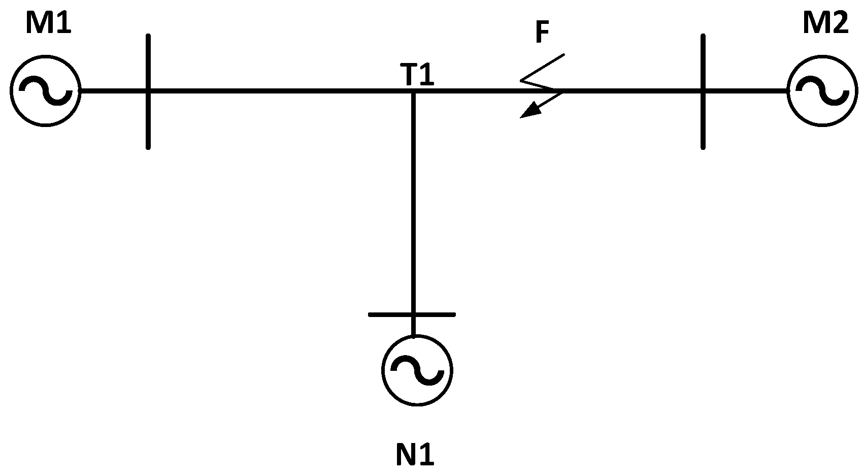
4.1. T-Type Transmission Line Fault Branch Judgment Method
When the T-type transmission line in Figure 4 experiences a failure, and the time for the fault traveling wave to reach each endpoint is , , .

Figure 4.
T transmission line.
There are two cases of faults on T-type transmission lines: faults on branch lines and faults on T nodes. These are discussed separately in this paper.
4.1.1. Fault Occurred on The Branch Line
As shown in Figure 4, the fault occurs on M1–M2 and the fault distances of branches M1–M2 and M1–N1 with M1 as the starting point are calculated according to (11).
Similarly, we can calculate the fault distance starting from M2 as and , and starting from N1 as and .
To further determine the location of the fault on the branch line, the calculated fault distance and the distance from the beginning of the branch line to the T node are used to construct a fault branch line judgment matrix, where × represents elements that are not considered.
The fault branch judgment matrix constructed by modeling the T-shaped transmission line in Figure 4 is given in Equation (26).
when the fault occurs on , , , , , ,, therefore, the fault branch judgment matrix is
As can be seen from the fault branch judgment matrix (27), the elements in the row corresponding to the M2 endpoint are all <0, while the elements in the column corresponding to the M2 endpoint are all >0. Therefore, the principle for determining the fault branch on a T-type transmission line is as follows: when the elements in the row of a fault branch judgment matrix corresponding to an endpoint are all <0 and the elements in the column corresponding to the same endpoint are all >0, then the endpoint corresponds to the fault branch.
4.1.2. T-Node Failure
When the fault occurs in the T-node, the distance from the fault point to any endpoint is the distance from the T-node to each endpoint, and all elements in the fault branch judgment matrix are 0. Therefore, the principle for determining a fault at the T-node of a T-type transmission line is as follows: when all elements in the fault branch judgment matrix are 0, the T-node is determined to be faulty.
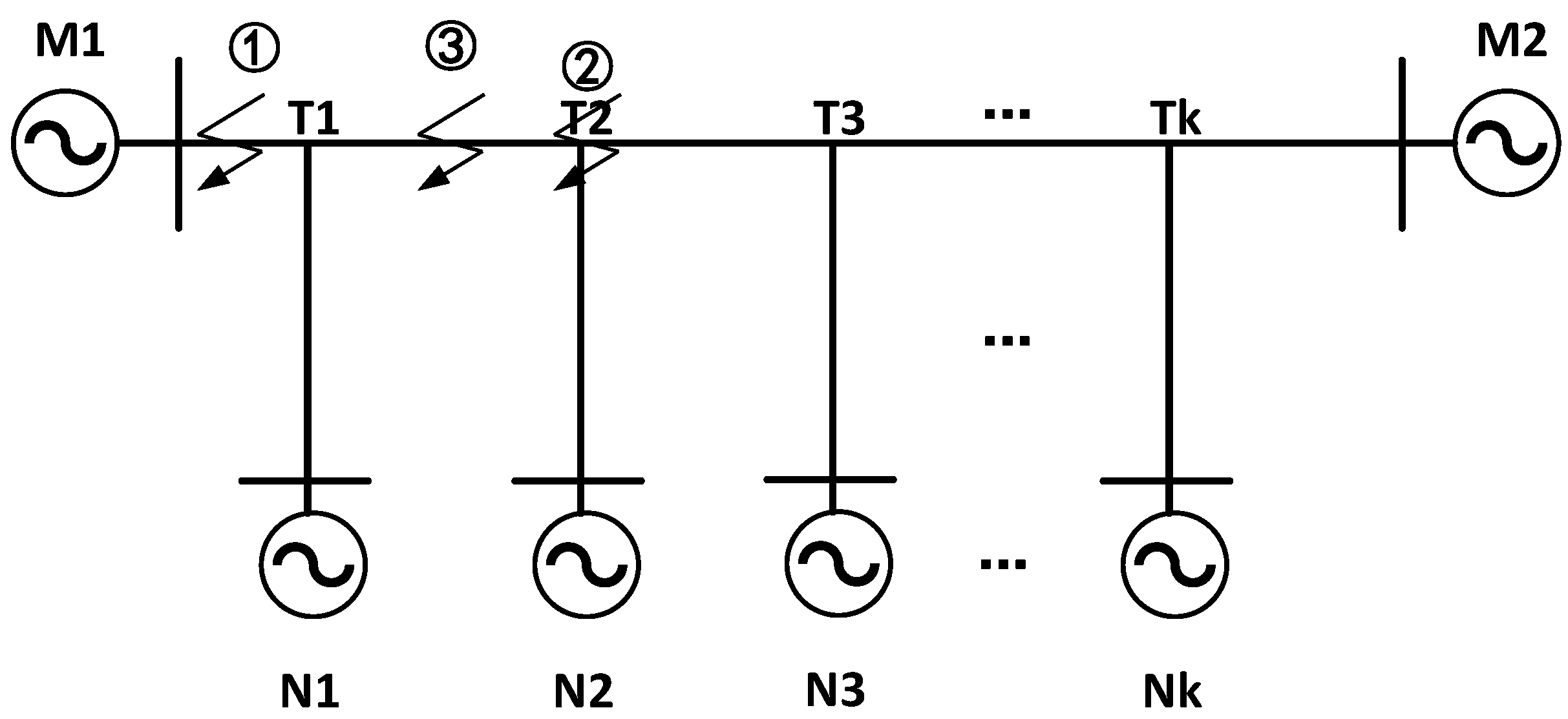
4.2. Multi-Terminal Transmission Line Fault Location Method
When a fault occurs in a multi-terminal transmission line that passes through multiple T-nodes, it can be analyzed using the T-type transmission line fault branch determination method proposed in the previous section. The schematic is shown in Figure 5.

Figure 5.
Multi-branch grid-connected line.
Multi-terminal transmission lines have multiple branch nodes. The corresponding element in the fault branch judgment matrix must be changed to the difference between the distance from the beginning to the fault point and the distance between the beginning of the fault branch and the nearest T-node from the end. Therefore, the fault branch judgment matrix is as follows:
There are three cases of multi-terminal transmission line faults: faults occurring on branch lines, T-node faults, and T-T inter-node faults. These are analyzed separately below.
4.2.1. Branch Line Failure
When a fault occurs in a branch line, as shown in Figure 5 (①), the fault occurs on M1–T1, which is thought to start from M1. The following relationship holds:
where, , I ∈ (1,2,3..., k), represents the endpoints of each branch line, and , I ∈ (1,2,3..., k) denotes each T node.
Therefore, the fault branch judgment matrix is as follows:
Combining Equations (29) and (30) yields the principle for determining the fault branch on a multi-branch grid-connected line. When the elements in a row of the fault branch judgment matrix are <0 and the corresponding elements in the column are >0, then the endpoint corresponding to the branch can be determined.
4.2.2. T-Node Failure
When a fault occurs at the T node, as shown in Figure 5 (②), the fault occurs at the T2 node. Similarly, the fault branch judgment matrix can be calculated as follows:
In Equation (31), the column elements corresponding to N2 are all equal to 0, and the row elements are all less than 0. Therefore, the principle of determining a fault at the T node is as follows: when the column elements corresponding to a specific endpoint in the fault branch judgment matrix are all equal to 0. The row elements are all less than 0, the fault is determined to occur in the branch node where the branch endpoint is located.
4.2.3. T-T Inter-Node Failure
When the fault occurs at nodes T1-T2, as shown by ② in Figure 5, the same principle of determination can be applied as follows: when the value of the line element corresponding to only one end measurement point in the fault branch judgment matrix is less than 0, and either only the value of the first element in its previous line is equal to 0 or only the last element in the next line is equal to 0, the fault is determined to occur between the T node of the branch where the endpoint is located and the T node corresponding to the endpoint in the previous or next line.
4.3. Fault Distance Calculation
A fault branch is defined according to the above principle by putting the line’s beginning at the fault point so that it forms the most double-ended branch endpoint, calculating the initial distance from the fault point to the other nodes in the double-ended branch, and finally calculating the average distance between these faults.
Using the average fault distance as the final result helps to cancel out positive and negative errors when multiple fault distances are calculated with both positive and negative errors, resulting in a more accurate positioning result. At the same time, taking the average value can also produce a compromise positioning result without a large error when the error of the calculated fault distance has the same sign.
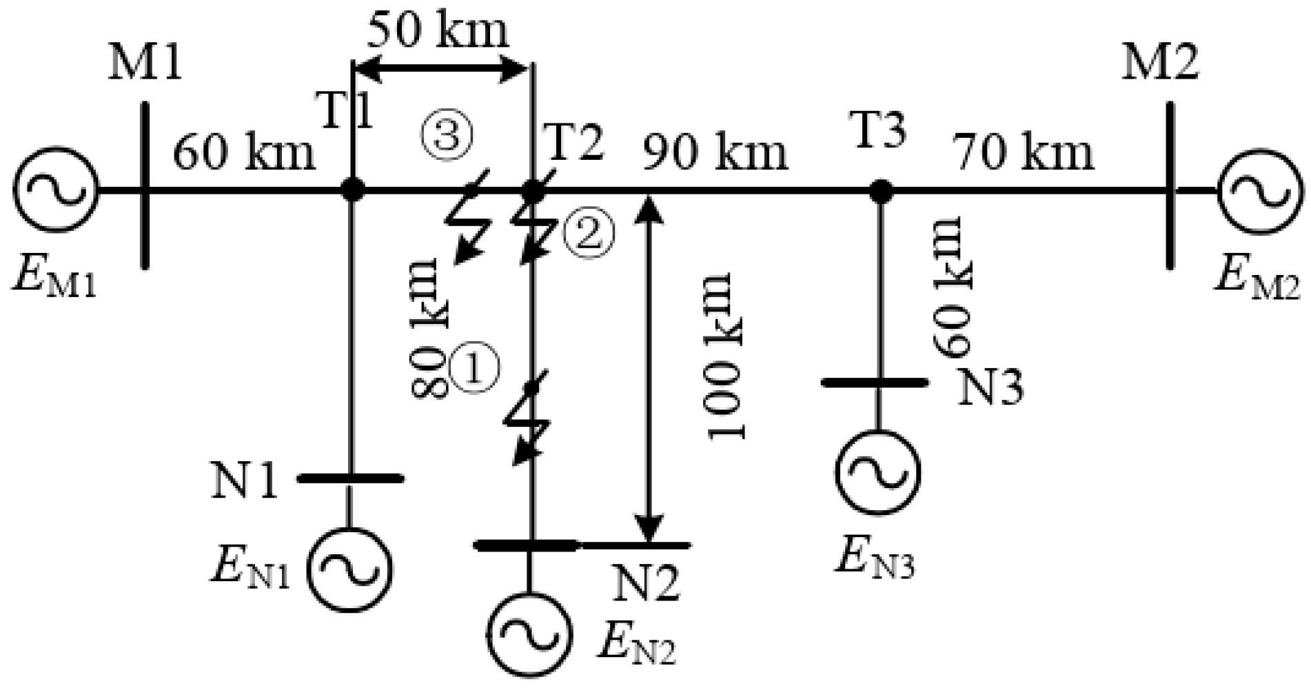
4.4. Simulation Verification
The 220 kV multi-branch grid-connected circuit shown in Figure 6 was built in ATP/EMTP. All line parameters are set to be the same, the sampling frequency is 10 MHz, and the fault occurrence time is 2 μs. The line parameters are highlighted in Table 3.

Figure 6.
Multi-terminal transmission line fault model.

Table 3.
Parameters of multi-branch grid-connected lines.
4.4.1. Branch Line Failure
As shown in Figure 6, a fault occurs at the N2 -T2 branch 40 km from the N2 end of the line, and the line wave signal is obtained at each end of the line using a line wave sensor. The signal is subjected to symmetric component transformation to obtain the line mode component. The initial wave heads of the faulty traveling wave mode components are calibrated using the modified CEEMDAN-TEO to obtain the time of arrival of the α-mode and β-mode components at each end of the fault, as shown in Table 4.

Table 4.
Time for the line modulus component to reach each endpoint.
The fault branch judgment matrix was constructed according to Equation (11)
it can be seen that the elements in the row corresponding to N2 are all less than zero, and the elements in the column corresponding to N2 are all greater than zero. This is consistent with the principle for determining a fault on a branch line proposed above, so it can be determined that the faulty branch is the branch where the N2 endpoint is located.
The fault distance using the N2 end as the initial end can be calculated as:
This shows that the faulty branch is accurately judged, and the positioning error is 177 m.
4.4.2. T-Node Failure
When a fault occurs at node T2, the time for the line mode components to reach each endpoint is shown in Table 5. A fault branch judgment matrix is then constructed.

Table 5.
Sampling numbers that the initial wave arrives at each measurement when the fault occurs on a T node.
Construct the fault branch judgment matrix according to Equation (11)
From Equation (36), the row elements corresponding to N2 are all less than zero. The column elements are all equal to zero, consistent with the T-node fault determination proposed above. Thus, the fault point can be identified as the T2 node.
To calculate the fault distance using the N2 end as the initial end, the following is obtained:
This demonstrates that the fault point has been accurately determined, with a positioning error is 102 m.
4.4.3. T-T Failure
In the case of a T-T failure, the time for the line mode components to reach each endpoint is shown in Table 6, and a fault branch judgment matrix is constructed.

Table 6.
Sampling numbers that the initial wave arrives at each measurement when the fault occurs on a T node.
The fault branch judgment matrix can be constructed according to Equation (11)
From Equation (36), the elements of the rows corresponding to N2 are all less than zero. According to the T-node fault determination proposed above, only the first element of the N1 row is zero, so the fault point can be determined between T1 and T2.
Calculate the fault distance using the N2 end as the initial end.
In order to further verify the accuracy of the distance measurement method proposed in this paper, a comparison was made using the technique in this paper and the method in Zeng et al. []. The results of the comparison are shown in Table 7 and Table 8.

Table 7.
The results of the method presented in this paper are obtained under different experimental conditions.

Table 8.
The results of reference [] under different experimental conditions.
Due to space constraints, the results of all comparative experiments are not listed in this paper. However, the comparison results show that the method proposed in this paper is superior to the method by Zeng et al. [] in terms of distance measurement error, fault branch judgment, and calculation speed. It has a high positioning accuracy and is suitable for use in actual working conditions.
5. Conclusions
To address the problem of fault location in multi-branch grid-connected lines, this paper proposes a CEEMDAN-TEO-based fault ranging method for multi-terminal transmission lines. This method combines CEEMDAN and TEO to accurately extract fault mutations under strong noise interference and accurately capture fault-traveling waveheads, providing a foundation for subsequent accurate fault location. The traditional double-ended weakness-ranging algorithm is also improved by proposing a double-ended ranging method based on line mode components, which eliminates the influence of line wave speed uncertainty on fault-ranging results. This method does not need to consider line wave fold reflection or fault occurrence time.
For fault branch determination in multi-terminal transmission lines, this paper constructs a fault branch determination matrix based on the difference between the fault transmission distance and the line branch length. It combines the traveling wave head capture method and the improved double-end fault ranging form to achieve accurate fault location. It compares it to the current multi-terminal transmission line location method to achieve precise fault branch determination. The proposed method can achieve accurate fault branch determination and high-ranging accuracy, meeting the requirements of actual working conditions.
Author Contributions
Conceptualization, Q.Z. and Y.Y.; methodology, M.W. and X.W.; software, M.W.; validation, M.W., E.Q.; formal analysis, X.W.; investigation, Y.Y; data curation, X.W. and E.Q.; writing—original draft preparation, Q.Z.; writing—review and editing, Y.Y. and Q.Z.; visualization, E.Q. All authors have read and agreed to the published version of the manuscript.
Funding
This research was supported by [Jilin Province Science and Technology Development Program Project], grant number [20220201075GX].
Institutional Review Board Statement
Not applicable.
Informed Consent Statement
Not applicable.
Data Availability Statement
The data used to support the findings of this study are included in the article.
Conflicts of Interest
The authors declare that they have no competing interests.
References
- Khoshbouy, M.; Yazdaninejadi, A.; Bolandi, T.G. Transmission line adaptive protection scheme: A new fault detection approach based on pilot superimposed impedance. Int. J. Electr. Power Energy Syst. 2022, 137, 107826. [Google Scholar] [CrossRef]
- Ortega, J.S.; Tavares, M.C. Fault impedance analysis and non-conventional distance protection settings for half-wavelength transmission line applications. Electr. Power Syst. Res. 2021, 198, 107361. [Google Scholar] [CrossRef]
- Dai, F.; Zeng, D.; Liu, S.; Wang, G. A practical impedance modeling method of MMC-HVDC transmission system for medium-and high-frequency resonance analysis. Electr. Power Syst. Res. 2022, 212, 108636. [Google Scholar] [CrossRef]
- Wang, D.; Cheng, D.; Sun, X.; Chen, W.; Qiao, F.; Liu, X.; Hou, M. Novel travelling wave directional pilot protection approach for LCC-MMC-MTDC overhead transmission line. Int. J. Electr. Power Energy Syst. 2023, 144, 108553. [Google Scholar] [CrossRef]
- Chen, W.; Wang, D.; Cheng, D.; Liu, X. Travelling wave fault location approach for MMC-HVDC transmission line based on frequency modification algorithm. Int. J. Electr. Power Energy Syst. 2022, 143, 108507. [Google Scholar] [CrossRef]
- Banafer, M.; Mohanty, S.R. A travelling wave based primary and backup protection for MMC-MTDC transmission system using morphological un-decimated wavelet scheme. Electr. Power Syst. Res. 2022, 212, 108367. [Google Scholar] [CrossRef]
- Mousaviyan, I.; Seifossadat, S.G.; Saniei, M. Traveling Wave-based Algorithm for Fault Detection, Classification, and Location in STATCOM-Compensated Parallel Transmission Lines. Electr. Power Syst. Res. 2022, 210, 108118. [Google Scholar] [CrossRef]
- Parsi, M.; Crossley, P.; Dragotti, P.L.; Cole, D. Wavelet based fault location on power transmission lines using real-world travelling wave data. Electr. Power Syst. Res. 2020, 186, 106261. [Google Scholar] [CrossRef]
- Ravesh, N.R.; Ramezani, N.; Ahmadi, I.; Nouri, H. A hybrid artificial neural network and wavelet packet transform approach for fault location in hybrid transmission lines. Electr. Power Syst. Res. 2022, 204, 107721. [Google Scholar] [CrossRef]
- Rezaei, D.; Gholipour, M.; Parvaresh, F. A single-ended traveling-wave-based fault location for a hybrid transmission line using detected arrival times and TW′ s polarity. Electr. Power Syst. Res. 2022, 210, 108058. [Google Scholar] [CrossRef]
- Chen, W.; Wang, D.; Cheng, D.; Qiao, F.; Liu, X.; Hou, M. Novel travelling wave fault location principle based on frequency modification algorithm. Int. J. Electr. Power Energy Syst. 2022, 141, 108155. [Google Scholar] [CrossRef]
- Malik, H.; Fatema, N.; Iqbal, A. Intelligent Data-Analytics for Condition Monitoring: Smart Grid Applications; Academic Press: Cambridge, MA, USA, 2021; pp. 115–140. ISBN 9780323855105. [Google Scholar]
- Xie, L.; Luo, L.; Ma, J.; Li, Y.; Zhang, M.; Zeng, X.; Cao, Y. A novel fault location method for hybrid lines based on traveling wave. Int. J. Electr. Power Energy Syst. 2019, 141, 108102. [Google Scholar] [CrossRef]
- Abbasi, F.; Abdoos, A.A.; Hosseini, S.M.; Sanaye-Pasand, M. New ground fault location approach for partially coupled transmission lines. Electr. Power Syst. Res. 2023, 216, 109054. [Google Scholar] [CrossRef]
- Khalili, M.; Namdari, F.; Rokrok, E. Traveling wave-based protection for SVC connected transmission lines using game theory. Int. J. Electr. Power Energy Syst. 2020, 123, 106276. [Google Scholar] [CrossRef]
- Jamali, S.; Mirhosseini, S.S. Protection of transmission lines in multi-terminal HVDC grids using travelling waves morphological gradient. Int. J. Electr. Power Energy Syst. 2019, 108, 125–134. [Google Scholar] [CrossRef]
- Anane, P.O.K.; Huang, Q.; Bamisile, O.; Ayimbire, P.N. Fault location in overhead transmission line: A novel non-contact measurement approach for traveling wave-based scheme. Int. J. Electr. Power Energy Syst. 2021, 133, 107233. [Google Scholar] [CrossRef]
- Wang, D.; Hou, M. Travelling wave fault location principle for hybrid multi-terminal LCC-VSC-HVDC transmission line based on R-ECT. Int. J. Electr. Power Energy Syst. 2020, 117, 105627. [Google Scholar] [CrossRef]
- Reis, R.L.; Lopes, F.V. Correlation-based single-ended traveling wave fault location methods: A key settings parametric sensitivity analysis. Electr. Power Syst. Res. 2022, 213, 108363. [Google Scholar] [CrossRef]
- Zeng, R.; Wu, Q.; Zhang, L. Two-terminal traveling wave fault location based on successive variational mode decomposition and frequency-dependent propagation velocity. Electr. Power Syst. Res. 2022, 213, 108768. [Google Scholar] [CrossRef]
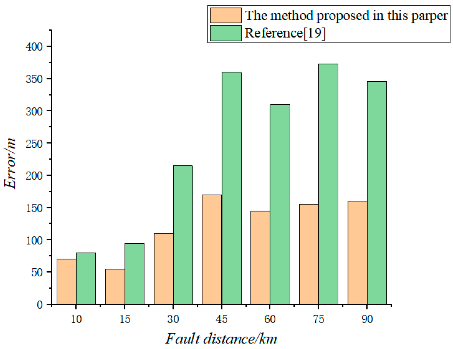
Disclaimer/Publisher’s Note: The statements, opinions and data contained in all publications are solely those of the individual author(s) and contributor(s) and not of MDPI and/or the editor(s). MDPI and/or the editor(s) disclaim responsibility for any injury to people or property resulting from any ideas, methods, instructions or products referred to in the content. |
© 2023 by the authors. Licensee MDPI, Basel, Switzerland. This article is an open access article distributed under the terms and conditions of the Creative Commons Attribution (CC BY) license (https://creativecommons.org/licenses/by/4.0/).