Article

DLALoc: Deep-Learning Accelerated Visual Localization Based on Mesh Representation

School of Computer and Information Security, Guilin University of Electronic Science and Technology, Guilin 541004, China
*
Author to whom correspondence should be addressed.
Appl. Sci. 2023, 13(2), 1076; https://doi.org/10.3390/app13021076
Submission received: 4 November 2022 / Revised: 5 January 2023 / Accepted: 5 January 2023 / Published: 13 January 2023

Abstract

:
Visual localization, i.e., the camera pose localization within a known three-dimensional (3D) model, is a basic component for numerous applications such as autonomous driving cars and augmented reality systems. The most widely used methods from the literature are based on local feature matching between a query image that needs to be localized and database images with known camera poses and local features. However, this method still struggles with different illumination conditions and seasonal changes. Additionally, the scene is normally presented by a sparse structure-from-motion point cloud that has corresponding local features to match. This scene representation depends heavily on different local feature types, and changing the different local feature types requires an expensive feature-matching step to generate the 3D model. Moreover, the state-of-the-art matching strategies are too resource intensive for some real-time applications. Therefore, in this paper, we introduce a novel framework called deep-learning accelerated visual localization (DLALoc) based on mesh representation. In detail, we employ a dense 3D model, i.e., mesh, to represent a scene that can provide more robust 2D-3D matches than 3D point clouds and database images. We can obtain their corresponding 3D points from the depth map rendered from the mesh. Under this scene representation, we use a pretrained multilayer perceptron combined with homotopy continuation to calculate the relative pose of the query and database images. We also use the scale consistency of 2D-3D matches to perform the efficient random sample consensus to find the best 2D inlier set for the subsequential perspective-n-point localization step. Furthermore, we evaluate the proposed visual localization pipeline experimentally on Aachen DayNight v1.1 and RobotCar Seasons datasets. The results show that the proposed approach can achieve state-of-the-art accuracy and shorten the localization time about five times.

1. Introduction

Precise visual localization of 6-degree-of-freedom (DoF) camera poses within a known three-dimensional structure is one of the most important abilities in some modern intelligence systems, e.g., self-driving cars [1,2] and augmented or virtual reality systems [3,4]. Obtaining a centimeter-accurate 6-DoF pose in real time is essential to guarantee reliable and safe driving and ensure immersive experiences. In terms of accuracy, most state-of-the-art visual localization methods are structure-based [5,6,7,8]. These approaches deploy a coarse-to-fine way to generate 2D–3D correspondences between a feature point from the query image and a database 3D point; each 3D point has its local features in database images.
However, in these methods, both 2D–2D local feature mismatch of query feature and database image features and 2D–3D mismatch of a database feature and database 3D point will lead to wrong 2D–3D match of a query feature and database 3D point, especially in large scale scene, which contains millions of features and points to match. Therefore, generating robust matching pairs within a limited time is essential for some real-time visual localization algorithms. The general way to filter out mismatches is to apply a modern random sample consensus (RANSAC) framework, which utilizes a minimal solver for optimization [9,10,11].
Moreover, the database point cloud is usually generated from the structure-from-motion (Sfm) process and the scene is presented with this point cloud and images [12,13]. A dense 3D model scene representation [14,15,16] is a replacement for using sparse Sfm point clouds and images. This representation uses the mesh generated via multiview stereo, Lidar or depth map to represent the scene which is more flexible at feature point types because it does not need to match local features between database images to triangulate the 3D point cloud. The 3D point can easily be obtained from the depth map rendered from the mesh. More importantly, this rendering process will not provide wrong 2D–3D matches compared with the 3D point cloud from the Sfm model.
In this paper, we propose to take advantage of mesh-based scene representation to alleviate the complexity of the 2D–3D matching step. We use the pretrained multilayer perceptron (MLP) combined with homotopy continuation to solve the relative poses [17]. We also use the scale consistency of 2D–3D matches to perform efficient RANSAC to find the best 2D inlier set for the subsequential perspective-n-point (PnP) [18] localization step. The input of the MLP in our approach is five-feature correspondences, and the outputs from the MLP are their corresponding depths in the scene; however, the scale is different from the rendered depth map. Using this method to solve relative pose can calculate once quickly. We employ scale consistency to verify whether a solution from the minimal RANSAC sample is a real solution or whether the input of MLP contains outliers to skip the validation step for some wrong solutions, which greatly improves the efficiency of RANSAC implementation.
The core idea of our approach is summarized as follows. With the mesh-based scene representation, the 2D–3D matches contain no mismatch. We use the pretrained MLP combined with homotopy continuation to calculate the relative pose in a short time. We also use the scale information from rendered 2D–3D correspondences to help the RANSAC to perform more efficiently. In such a way, we can get more robust 2D–2D correspondences in a short time. Thus, the 2D–3D matches established by these 2D features are also more robust. The performance of the algorithm can be greatly improved using such an approach.

2. Related Work

The 6 DoF visual localization has been widely studied in recent years. It can be classified into structure-based [5,6,7,8] and image-based approaches [19,20,21,22,23]. The structure-based approach normally triangulates feature correspondences from the database images to generate a 3D point cloud and represents the scene using this point cloud and database images. Each 3D point has its corresponding local features in the database images to match. In the test process, the 2D–3D matches are established between the local features in a query image and database point cloud using descriptor matching. Then, a PnP method based on these matches is used to localize the query image. Moreover, a hierarchical approach [5,8] is often used to handle different illumination conditions, seasonal changes, and large scenes with numerous database images. In most hierarchical localization pipelines, first, an image retrieval [24,25] stage is used to select the most relevant database image set for feature matching. The selected images range from 10 to 50, depending on different conditions. The 3D points for localization are often restricted to being visible in these images. Second, the 2D–3D matches of query features and database 3D points are established via explicit descriptor matching. Finally, the query pose can be obtained based on these matches. Meanwhile, the image-based approaches represent the 3D geometry implicitly by the weights of a machine learning model. Refs. [22,26,27,28,29] adopt the scene coordinate regression techniques, which use the neural network to regress the 2D–3D matches instead of computing them via explicit descriptor matching. There are also some techniques use the network to be a pose regressor. Refs. [19,20,21,30,31] use the network to regress the absolute poses, and [32,33] choose to regress the relative pose from a known database image. Though these scene coordinate regressors achieve state-of-the-art results for small scenes, the pose calculated from these methods are not competitive with the structure-based methods in more challenging scenes, even when [31,34] use the new view synthesis technology to generate more images for training the network.
Generally, the 3D point cloud used for scene representation is sparse and is generated from Sfm. One 3D point normally has many local features to match in different database images. For a large scene with millions of 3D points and many more 2D features, the mismatch of a 2D feature and 3D point is unavoidable when generating the point cloud. A covisable filtering [35,36] can reduce the mismatches by removing the 3D points that might not be visible together. Additionally, RANSAC can help to calculate the poses and find the best solution with maximal data support.
A dense 3D model [14,15,16] is an alternative to sparse point clouds and database images for scene representation. Different dense types ranging from dense multi-view stereo and laser point clouds to colored or textured meshes, have been used to represent the scene. Different from [15], which is mainly focused on coarse image localization (on the level of hundreds of meters), ref. [14] proposed a full pipeline to centimeter-accurate image localization based on mesh representation. This mesh-based method is still structure-based and obtains the 3D points from the depth map rendered from the mesh. Moreover, using the mesh to establish 2D-3D correspondences in runtime is more lightweight for memory usage than storing the whole Sfm model and images [14].
However, no matter which forms represent the scene, the final step of localization is to perform a RANSAC-based PnP solver for pose estimation. In each iteration, it samples a minimal set of 2D-3D correspondences to calculate pose. This step is time-consuming because it requires many iterations to refine the optimal solution from the noisy data. Therefore, the robustness of 2D–3D matches used to calculate relative pose is essential to improve the performance of the localization algorithm. For the mesh-based scene representation, establishing robust 2D–3D matches mainly depends on finding robust 2D feature correspondences. Nearest neighbors (NN) [37] is the most widely used feature matching method. The initial matches can be refined by following the RANSAC implementation. Ref. [38] proposed a learning-based feature matching strategy that can achieve high accuracy by performing a self/cross attention mechanism; however, this approach is more time-consuming compared with [37]. Ref. [17] proposed a novel learning-based method to solve the relative pose. Although the relative pose estimation is not required for the structure-based visual localization, this learning-based method can calculate once in a very short time. With this advantage, a more efficient RANSAC framework can be used to filter the outliers of 2D feature correspondences, thus improving the performance of visual localization algorithms.

3. System Illustration

Figure 1 shows the differences between the general hierarchical localization method and DLALoc method. Dark blue and cyan flow is the method proposed by [5]. In this method, the last step of estimating a query image pose is based on the P3P method [39]. Using RANSAC to perform robust pose estimation inside a P3P method is the most time-consuming step in the whole pipeline of this visual localization method. In order to release the burden of this step, we proposed DLALoc, which is illustrated as dark blue and yellow flow. Same as [5], DLALoc is still structure-based and the first step is to retrieve the most relevant database images. Then, the 2D–2D feature correspondences are calculated through some feature matching strategies. Different from [5], we do not obtain these 2D–2D correspondences directly from these feature matching strategies, which contain many outliers. Instead, we use a pretrained MLP that models the 3D structure of the scene to filter outliers of 2D feature correspondences, thereby establishing more robust 2D-3D matching pairs in the next step. The filtration of outliers is based on optimal relative pose estimation of two images (i.e., a query image and a database image) with RANSAC. We find the maximum 2D correspondence set whose reprojection error on another image according to epipolar constraint is under the threshold. Moreover, by using the mesh to represent the scene, we could obtain the 2D–3D matching pairs from the rendered depth map, and these 2D–3D matching pairs are more precise than Sfm model. Thus, we take advantage of this property, and propose to use the scale consistency to a step further help us to filter out the outliers. To be specific, the different depth information of five 2D–3D matching pairs between the depth map and output from the MLP can give a preknowledge of whether the relative pose has been accurately calculated or the input to calculate the relative pose contains outliers. In this way, we can skip the inner validation step of some wrong solutions to perform a more efficient RANSAC and obtain robust 2D correspondences in a short time.
As illustrated above, in DLALoc method, because the 2D information can be handled more efficiently, we split the RANSAC in the P3P method into two steps. In the first step, we used RANSAC to filter 2D outliers. In the second step, RANSAC is used for robust pose estimation whose inputs contain less noise. The first RANSAC step was much more efficient than the second step. Therefore, the entire visual localization algorithm can be greatly improved in terms of efficiency and accuracy.

4. Methods and Material

4.1. Mesh-Based Visual Localization

In this section, we first introduce the hierarchical mesh-based visual localization algorithm, which is mainly divided into four steps:
Step 1: Image retrieval. Given a query image, a coarse search at the image level is performed to find the most relevant views in the database. This is done by matching the global descriptors of images, and the top-k NN are selected as the prior images. This step is efficient given that there can be far fewer images to match in the database.
Step 2: Local feature matching. This step generates the 2D–2D local feature correspondences between the query and top-k retrieved database images. These 2D–2D correspondences will be lifted to the 2D–3D matches in the next step. It is common to use state-of-the-art deep-learning local features. Additionally, local features can be matched by exhaustive matched or deep-learning matching strategies.
Step 3: Lift local feature correspondences to 2D–3D matches. Since we can get the depth map by rendering the mesh, each feature f i j (where i indicates the image index, and j indicates the feature index) has a valid depth in the scene, and the 3D points P i can be recovered from the depth. There are only some noisy 2D feature measurements which will be propagated to 3D points (i.e., even though f 1 j , f 2 j ... corresponding to the same 3D point in the physical world, the corresponding 3D points recovered from the depth map will be slightly different). There is no mismatch of 2D–3D matches in the SFM model (i.e., f 1 j , f 2 k ... corresponding to the different 3D points but was categorized to be the same projection of a 3D point), which greatly influences the efficiency and accuracy of the localization algorithm.
Step 4: Pose estimation: The last step is to use the resulting 2D–3D matches to calculate the image poses. The P3P method calculates the poses from the minimal sample of the three 2D–3D matches in each iteration, and the RANSAC framework is performed to refine the optimal estimation inside and after RANSAC with a nonlinear refinement for all inliers. Figure 2 shows the mesh-based scene representation.

4.2. Learning-Based Relative Pose Estimation

Relative pose estimation is not required in the above method. Because regressing the query pose from the database views is inaccurate, as estimating the pose from structure-based methods contains consistency checks within a RANSAC. However, in our method we use the relative pose estimation mechanism as a strong outlier filter, which greatly improves the efficiency and accuracy of the localization algorithm.
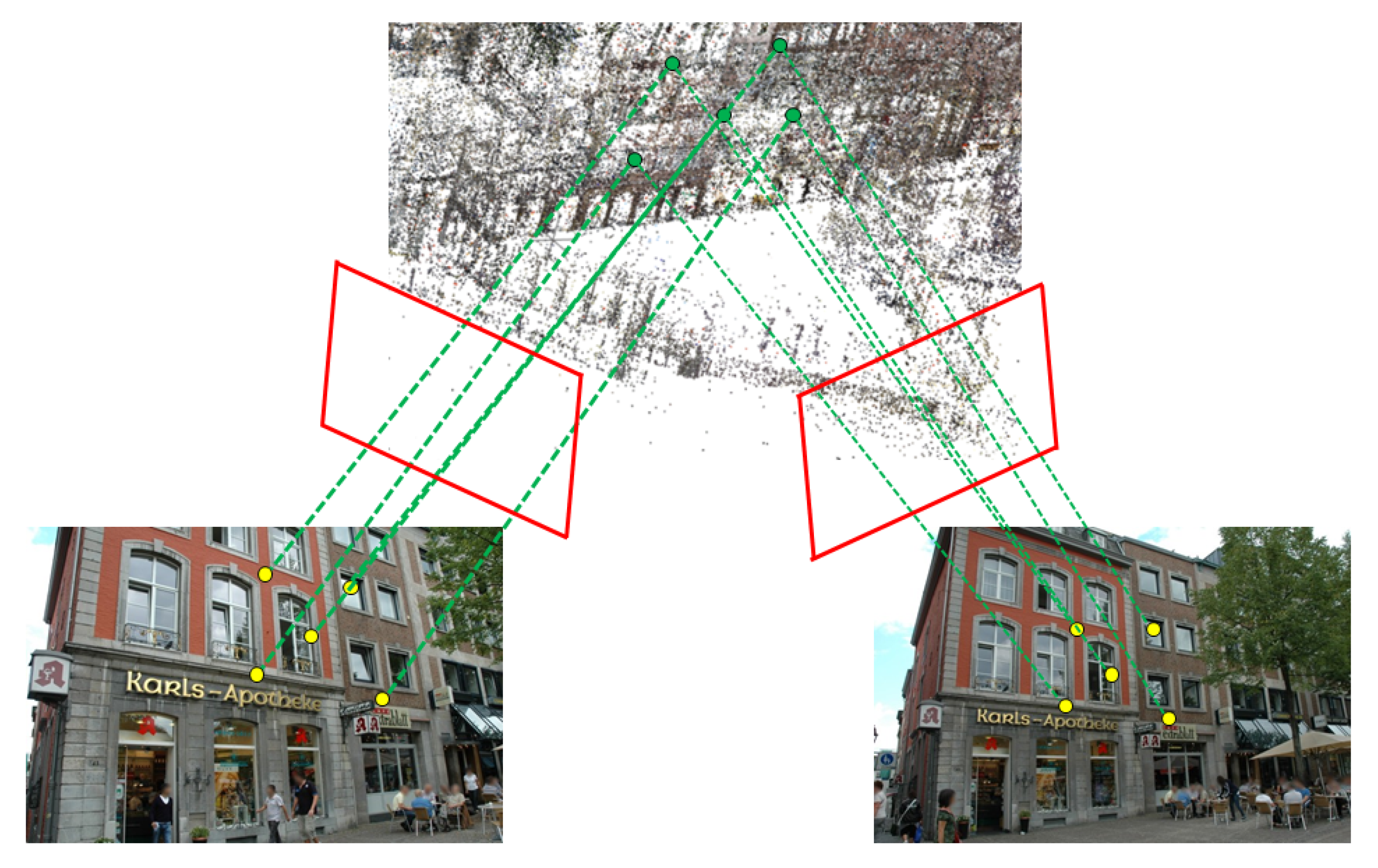
Ref. [17] proposed a deep-learning method to estimate the relative pose of two images, which is also feature-based same as the five-point method [40]. Due to geometry consistency, as illustrated in Figure 3, the distance between every two 3D points, when reconstructed in different cameras, must be the same. Thus, the form of a five-point problem in this method is parametrized by the projection of five 3D points into 2 calibrated cameras. There are ten unknown depths of five 3D points in two images λ k , i , k = 1 , . . . , 5 , i = 1 , 2 , and the result can be solved by 10 = 5 2 equations given in (1):
λ k , i v k , i λ m , i v m , i 2 = λ k , j v k , j λ m , j v m , j 2
where λ k , i , λ k , j , λ m , i , λ m , j are two features correspondences, and v k , i , v k , j , v m , i , v k , i are their depths in the scene.
We also use deep-learning to solve this problem. We first extract pairs of five local feature correspondences and their ten corresponding depths from the SFM model to be the training data. In this paper, we call this form of pair a n c h o r s . We choose a certain number of anchors with the best connectivity to be the output of MLP.
At test time, with arbitrary five local feature correspondences selected from the query image and database image as inputs, the MLP can find which anchor has the nearest geometry to track according to the input local features. It will also track this anchor with homotopy continuation to output the depth of these ten local features. Then, the coordinates of local features and their depths in the scene can be decomposed into the relative pose with a unique solution. Figure 4 shows the entire pipeline of this algorithm.
There are several reasons why we incorporate this relative pose estimating stage. First, estimating relative pose using MLP combined with homotopy continuation has orders of magnitude advantage of time compared with other methods (calculating time is on the level of µs) and time spent on adding additional relative pose estimation is negligible in the entire algorithm. Moreover, the nearest anchors and training data are extracted from the Sfm model. Therefore, we can model the 3D structure of the scene with MLP.
Second, the solution was tracked from the anchors extracted from the SFM model. Therefore, we can directly obtain the depths of the local features in the 3D structure, where the depths are in a convenient format for the validation step of our localization algorithm.
Third, this network is lightweight and thus easy to train. It can easily generate training data. Therefore, we can customize this neural network for different scenarios to improve the performance of finding the real geometry. We train our MLP using data extracted from Aachen DayNight v1.1 and RobotCar Seasons datasets. We also compared the performance under the Aachen DayNight v1.1 (Table 1). Here, Aachen/RobotCar Seasons [%] indicates the success ratio of finding the real geometry with MLP trained on two different datasets. We can see that the success ratio of MLP trained on the Aachen DayNight v1.1 dataset is nearly twice as good as that on the RoborCar Seasons dataset.

4.3. Efficient RANSAC Using Scale Consistency

With the mesh-based scene representation, we can use the depth from the projection of the mesh to verify whether the solution from MLP combined with homotopy continuation is the real geometry or the input of MLP contains outliers.
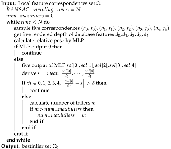
To be more specific, in this step, the input of the MLP is five local feature correspondences in the query and database images. We denote the five local features in the database image as f 0 , f 1 , f 2 , f 3 , and f 4 . We denote their corresponding depth in the depth map as d 0 , d 1 , d 2 , d 3 , and d 4 . The output of the MLP is ten depths of these five feature correspondences (five depths for the database image and five for the query image), whose scale is different from the depth map. We denote the output of the five depths in the database image as Sol [ 0 ] , Sol [ 1 ] , Sol [ 2 ] , Sol [ 3 ] , and Sol [ 4 ] . Suppose the MLP has tracked the correct geometry with the correct input; the five depths obtained from five depth maps and MLP, ideally, only differ a scale factor (i.e., for i { 0 , 1 , 2 , 3 , 4 } , the ratio of d i and Sol [ i ] should be the same). Therefore, we set a deviation threshold for Sol [ i ] d i , i { 0 , 1 , 2 , 3 , 4 } considering the noise. If there exists a ratio that is obviously different from others, we suppose it is an unreal solution. Thus, we can skip the validation step of this solution in the inner loop of RANSAC, which greatly improves the efficiency of RANSAC. We illustrate our algorithm to filter out 2D outliers in Algorithm 1.
Algorithm 1 Filtration algorithm using scale consistency
Applsci 13 01076 i001

5. Experimental Evaluation

5.1. Experiment Prerequisites and Dataset

In this section, we validate both the accuracy and efficiency of our DLALoc localization algorithm on two large scene datasets namely Aachen Day-night v1.1 and RobotCar Seasons. We also examine how the number of anchors and different RANSAC sampling times of our additional RANSAC implementation affect the algorithm’s performance. The Aachen Day-Night v1.1 dataset contains 6697 database images captured in an old European town, Aachen, Germany. All database images were taken under daytime conditions over different seasons. This dataset also contains 824 daytime and 191 nighttime query images captured with different mobile devices. We use both daytime and more challenging nighttime images for evaluation. The RobotCar Season datasets is a benchmark dataset for long-term autonomous driving localization. The images were taken on an urban road that spans multiple city blocks with the RobotCar platform. This dataset contains 20,862 overcast database images, and a total of 11,934 images for query taken under different conditions like sun, dusk, and rain. To generate the mesh model, we first use colmap [13] to generate sfm point cloud from stereo images; then, we use this multiview stereo point cloud to generate mesh by using screened Poisson surface Reconstruction [41]. All the testing experiments are conducted in Ubuntu version 18.04 operating system equipped with Intel® Core™ i7-7700 CPU @ 3.60 GHz × 8 CPU, NVIDIA GeForce RTX 3070 8 GB/PCIe/SSE4 Graphics, and 32 GB Memory.

5.2. Methods and Metrics

Training data preparation: The original SFM model of Aachen Day-Night contains too many database images to handle, and some 3D points have few 2D features in database images. We use the covisible graph to select the best covisible database images and 3D points to be the subset of the original SFM model for anchor extraction.
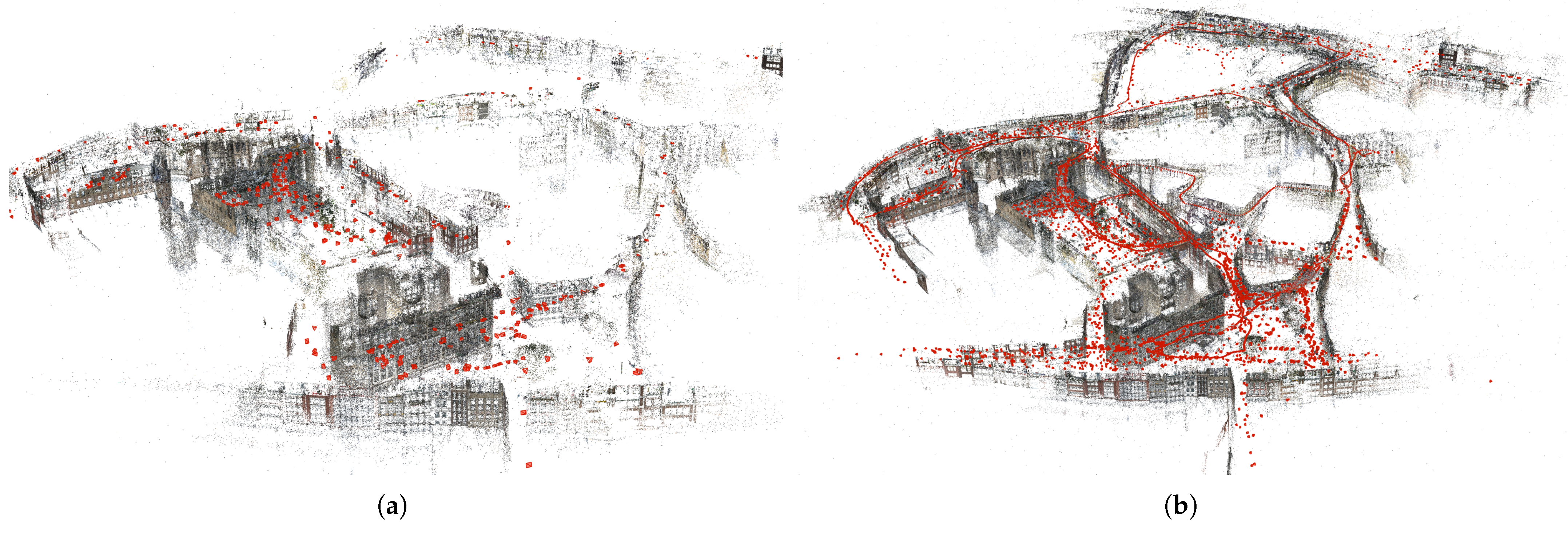
We define the covisible graph from the Sfm reconstruction as ( ( I 1 , I 2 ) , P ) , a bipartite graph where two nodes correspond to two database images ( I 1 , I 2 ) , and the edge P corresponds to the number of 3D points that are covisible in both images. In our experiment, we select 200 image pairs from the visible graph whose covisible edge is greater than 150, and their covisible 3D points to a the simplified SFM model. Figure 5 compares the two Sfm models.
We first evaluate the performance of our localization algorithm to fit different global features, local features, and feature matching strategies. we conducted experiments on learned and traditional local features (SuperPoint [42] and SIFT [43]) based on images extracted by NetVLAD. Then, the features can be matched by NN [37] or SuperGlue [38] method. We call them NV+SP+NN, NV+SP+SG, NV+SIFT+NN, and NV+SIFT+SG. Next, we evaluate a more efficient method that simultaneously computes local and global features using HF-Net [5] on our method, with the same matching strategy. We call them HF-Net+NN and HF-Net+SG. We set different numbers of anchors and RANSAC sampling times to show how the different MLP and RANSAC parameters could affect the efficiency and accuracy of the localization algorithm.
Furthermore, we introduce the following metrics to evaluate the partial and global performances of the localization algorithm.
  • The overall accuracy of localization is defined by position and orientation error. The position error is defined as the Euclidean distance p e s t p g t 2 between the estimated pose p est , and ground truth pose p gt . The orientation error is the absolute degree error computed from the estimated and ground truth camera rotation matrices R e s t , R g t ; we derived error | ζ | from 2 cos | ζ | = trace ( R e s t 1 R g t ) 1 . Additionally, we calculate the percentage of query images localized within three error thresholds varying from high precision (0.25 m, 2°) to medium precision (0.5 m, 5°) to low precision (5 m, 10°).
  • Matching time is the time used to establish 2D–3D matches of query and database images. This time includes time spent on image retrieval, extracting local features of query images, and matching these features to retrieved database image features.
  • P3P time is the time used for P3P method as illustrated in Step 4; providing high quality 2D–3D matches can significantly reduce the time for this step.
  • P3P points are the average 3D points that localize a query image. The less number of P3P points that are used to reach a certain level of quality of the 2D–3D matches built on these 3D points for localization, the better the algorithm performance.
  • MLP time is the total time used for additional pose estimation combined with filtering 2D correspondence outliers. The reduction of time in our algorithm can be estimated by the decrease in P3P time plus additional time spent.

5.3. Experimental Results and Analysis

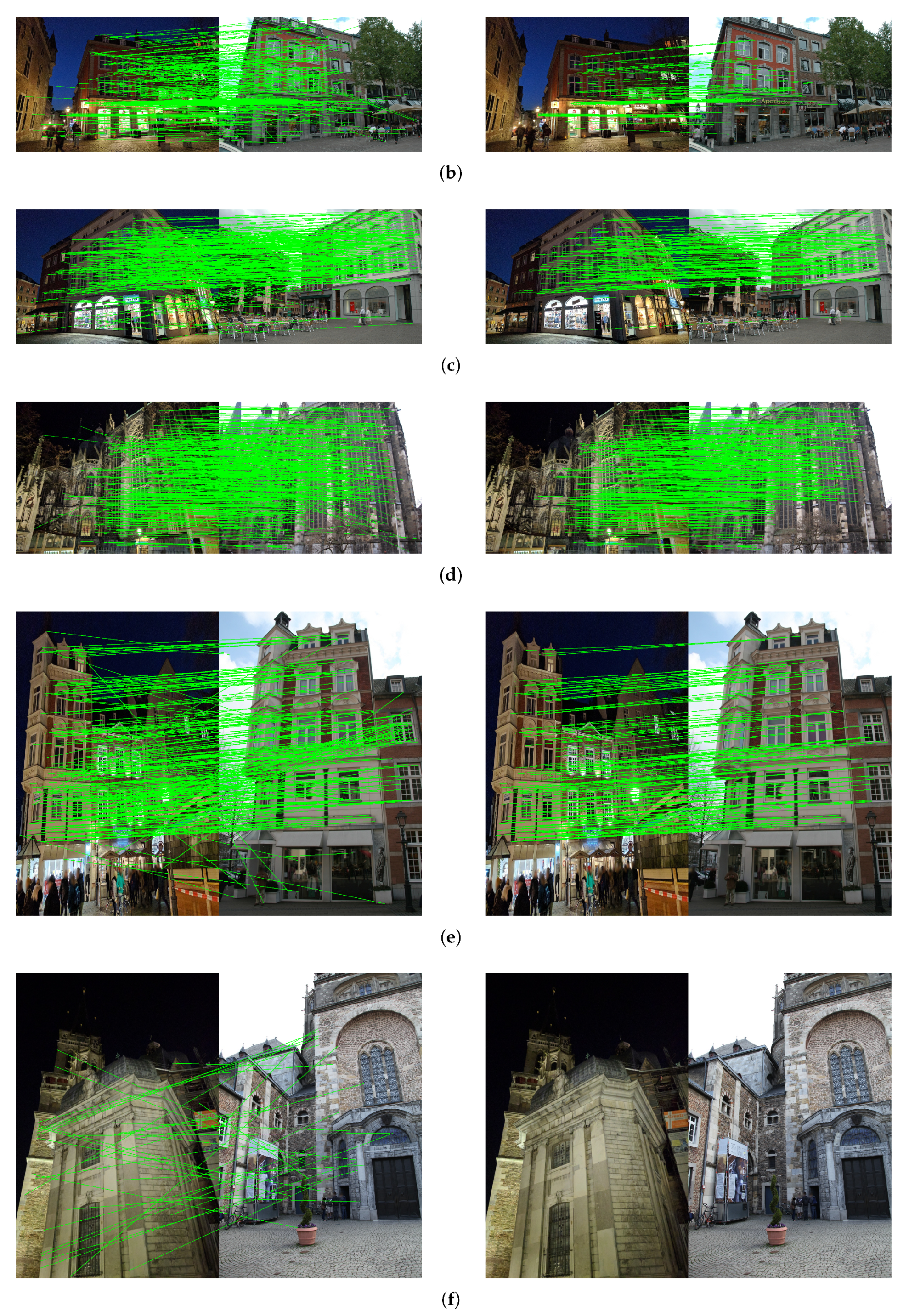
Table 2 presents the accuracy results of hierarchical localization method proposed by [5] on the Aachen and RobotCar Seasons datasets. We use the different combination of image retrieval, feature extraction, and matching strategies to localize a image as illustrated is Section 5.2. As presented in Table 2, we can see that on the Aachen dataset all methods in daytime queries outperform nighttime queries, and NV+SP+SG is the most competitive on all queries. The relatively poor performance in nighttime is mainly because that the nighttime condition suffers more error-prone feature correspondences than the daytime environment. Additionally, the learning-based feature types and matching strategies outperform the traditional methods. Table 3, Table 4 and Table 5 show the accuracy results of DLALoc with 100 anchors and different RANSAC sampling times using the same combinations of Table 3. Data with improvements compared to Table 3 are highlighted on black bold. The results show that our localization algorithm still maintains the trend on Table 3, confirming that our method can take advantage of the better image retrieval method as well as local feature types and matching strategies. When the RANSAC sampling times is greater than 50 our method can achieve more accurate results at all levels of precision. These improvements are more significant on the nighttime queries. This result further highlights the filtering effect of our method. However, when the RANSAC sampling time is 25, we only achieve a more precise result on the lowest precision level, meaning that the estimated pose is not so accurate that when filtering bad correspondences, some good matching pairs will also be filtered out along with bad ones. Furthermore, when the RANSAC sampling time is 100, the precision improvement is smaller than of the 50 RANSAC sampling time. This indicates that our RANSAC mechanism may converge around 50 sampling times. However, on the RobotCar Seasons dataset, our method performs similar to the Aachen dataset. On dusk and sun sequences, the accuracy tends to saturate. However, our method can achieve a more robust result in the more challenging sequences than all baselines when the RANSAN sampling time is greater than 50. Since the main advantage of DLALoc is that it can filter 2D outliers efficiently, we compare the different 2D feature correspondences of the same query image under baseline method and DLALoc with 100anchors and 50 RANSAC sampling times on Figure 6. As Figure 6 illustrated, DLALoc does filter out most of the outliers, which is the key to the improvement of localization algorithm.
Table 6 compares the overall time of DLALoc with 100 anchors and 50 RANSAC sampling times and the time it spends in separate parts with the baseline of three combinations on the Aachen dataset. The total localization time of these three methods differs from 20.4 to 35.6 mins. The time difference between these three methods mainly concentrates on the feature matching and P3P steps. We also improve the algorithm by putting the feature correspondences produced by these methods into the MLP and using the MLP to filter the outliers. We can see the total time of the improved NV+SP+NN method reduced from 35.6 to 6 min. However, it almost achieves the localization accuracy on all three levels of the original NV+SP+SG method. Moreover, we can see the total time of the improved NV+SP+SG method reduced from 20.4 to 4.6 mins, and we can still improve the localization accuracy. Moreover, HF-Net seems to be a compromise of efficiency and accuracy, which has the shortest matching time in all three baselines and can achieve relatively high accuracy. With our improvement, this combination can achieve outstanding efficiency and state-of-the-art accuracy.
As can be seen, our method has a significant time priority compared with the traditional method. This is mainly because the reduction of the P3P time is way beyond the additional time brought by the relative pose estimation and outlier filtration. The resulting P3P points are fewer; however, the 2D–3D matches are more robust. Although, some deep-learning matching strategies can provide more robust correspondences, they will bring additional space and time overhead. Meanwhile, we can use the fine filtration strategy to efficiently filter the outliers even with relatively poor matches as input, which can act as a substitute for expensive matching strategies. Moreover, from the 25 to 100 RANSAC sampling times, the additional time spent on calculating relative pose and filtering outliers is shorter than that of other algorithms. However, the total time for localization can be reduced significantly, and the accuracy can be improved from 50 RANSAC sampling times.
Furthermore, we train the MLP with different numbers of anchors as output to illustrate how the performance of the DLALoc algorithm can react to different anchor numbers. Figure 7 shows the algorithms’ accuracy and time on different anchor numbers. It can be clearly seen that the accuracy of calculating relative pose increases as the number of anchors increases. Interestingly, the runtime is not monotonic in the anchor number, and we can see the best performance occurs when the anchor number is 100. The reason is as follows. When the anchor is less than 100, the outliers cannot be effectively filtered out yet, so the 2D–3D matching pairs for localization still contain some outliers. When anchors are larger than 100, the filtration performance of MLP confronts a bottleneck and can be no longer improved, so the P3P time cannot be reduced, whereas the calculation time of MLP increases as anchors increase. Nevertheless, for all anchor numbers, the localization time is significantly less than the baseline time.

6. Conclusions

In this paper, we proposed a novel visual localization algorithm called DLALoc that is far more efficient and can still obtain more accurate results. Our system still follows a hierarchical localization pipeline [5]. In the proposed DLALoc algorithm, we use the mesh to represent the scene. Thus, we can obtain the 3D points from the rendered depth map, which is unique for one local feature in images. We also add the additional relative pose estimation step, which is not needed in the general hierarchical localization pipeline to filter outliers of 2D feature correspondences. Additionally, we perform local 2D-3D matching of the 2D inliers to obtain accurate 6-Dof poses.
Furthermore, we evaluated the proposed algorithm on different combinations of image-retrieval methods, local feature types, and feature matching strategies. The experimental results show that the proposed method can outperform state-of-the-art hierarchical methods with all combinations in terms of efficiency and accuracy. We further demonstrate how the better 2D correspondences can improve the performance of the localization algorithm by counting the time on different parts of the entire algorithm. The results show that the additional time on calculating the relative pose of the filtering outliers is trivial compared to the whole pipeline and significantly reduces the time of localizing with 2D–3D matches. Moreover, the total time for localization can be shortened by five times around and can still improve accuracy.

Author Contributions

Conceptualization, P.Z. and W.L.; methodology, P.Z.; software, P.Z.; validation, P.Z. and W.L.; formal analysis, P.Z.; investigation, P.Z. and W.L.; resources, W.L.; data curation, P.Z.; writing—original draft preparation, P.Z.; writing—review and editing, P.Z. and W.L.; visualization, P.Z. and W.L.; supervision, P.Z. and W.L.; project administration, W.L.; funding acquisition, W.L. All authors have read and agreed to the published version of the manuscript.

Funding

This work was supported by the National Natural Science Foundation of China under Grant 61862011.

Conflicts of Interest

The authors declare no conflict of interest. The funders had no role in the design of the study; in the collection, analyses, or interpretation of data; in the writing of the manuscript, or in the decision to publish the results.

References

  1. Liu, D.; Cui, Y.; Guo, X.; Ding, W.; Yang, B.; Chen, Y. Visual localization for autonomous driving: Mapping the accurate location in the city maze. In Proceedings of the 2020 25th International Conference on Pattern Recognition (ICPR), Milan, Italy, 10–15 January 2021; pp. 3170–3177. [Google Scholar]
  2. Bürki, M.; Schaupp, L.; Dymczyk, M.; Dubé, R.; Cadena, C.; Siegwart, R.; Nieto, J. Vizard: Reliable visual localization for autonomous vehicles in urban outdoor environments. In Proceedings of the 2019 IEEE Intelligent Vehicles Symposium (IV), Paris, France, 9–12 June 2019; pp. 1124–1130. [Google Scholar]
  3. Amato, G.; Cardillo, F.A.; Falchi, F. Technologies for visual localization and augmented reality in smart cities. In Sensing the Past; Springer: Berlin/Heidelberg, Germany, 2017; pp. 419–434. [Google Scholar]
  4. Middelberg, S.; Sattler, T.; Untzelmann, O.; Kobbelt, L. Scalable 6-dof localization on mobile devices. In Proceedings of the European Conference on Computer Vision, Zurich, Switzerland, 6–12 September 2014; pp. 268–283. [Google Scholar]
  5. Sarlin, P.E.; Cadena, C.; Siegwart, R.; Dymczyk, M. From coarse to fine: Robust hierarchical localization at large scale. In Proceedings of the IEEE/CVF Conference on Computer Vision and Pattern Recognition, Long Beach, CA, USA, 16–20 June 2019; pp. 12716–12725. [Google Scholar]
  6. Sattler, T.; Weyand, T.; Leibe, B.; Kobbelt, L. Image Retrieval for Image-Based Localization Revisited. In Proceedings of the BMVC, Surrey, UK, 3–7 September 2012; Volume 1, p. 4. [Google Scholar]
  7. Sarlin, P.E.; Unagar, A.; Larsson, M.; Germain, H.; Toft, C.; Larsson, V.; Pollefeys, M.; Lepetit, V.; Hammarstrand, L.; Kahl, F.; et al. Back to the feature: Learning robust camera localization from pixels to pose. In Proceedings of the IEEE/CVF Conference on Computer Vision and Pattern Recognition, Virtual, 19–25 June 2021; pp. 3247–3257. [Google Scholar]
  8. Humenberger, M.; Cabon, Y.; Guerin, N.; Morat, J.; Revaud, J.; Rerole, P.; Pion, N.; de Souza, C.; Leroy, V.; Csurka, G. Robust image retrieval-based visual localization using kapture. arXiv 2020, arXiv:2007.13867. [Google Scholar]
  9. Barath, D.; Ivashechkin, M.; Matas, J. Progressive NAPSAC: Sampling from gradually growing neighborhoods. arXiv 2019, arXiv:1906.02295. [Google Scholar]
  10. Barath, D.; Noskova, J.; Ivashechkin, M.; Matas, J. MAGSAC++, a fast, reliable and accurate robust estimator. In Proceedings of the IEEE/CVF Conference on Computer Vision and Pattern Recognition, Seattle, WA, USA, 13–19 June 2020; pp. 1304–1312. [Google Scholar]
  11. Chum, O.; Matas, J. Matching with PROSAC-progressive sample consensus. In Proceedings of the 2005 IEEE Computer Society Conference on Computer Vision and Pattern Recognition (CVPR’05), San Diego, CA, USA, 20–26 June 2005; Volume 1, pp. 220–226. [Google Scholar]
  12. Agarwal, S.; Furukawa, Y.; Snavely, N.; Simon, I.; Curless, B.; Seitz, S.M.; Szeliski, R. Building rome in a day. Commun. ACM 2011, 54, 105–112. [Google Scholar] [CrossRef]
  13. Schonberger, J.L.; Frahm, J.M. Structure-from-motion revisited. In Proceedings of the IEEE Conference on Computer Vision and Pattern Recognition, Las Vegas, NV, USA, 27–30 June 2016; pp. 4104–4113. [Google Scholar]
  14. Panek, V.; Kukelova, Z.; Sattler, T. MeshLoc: Mesh-Based Visual Localization. In Proceedings of the European Conference on Computer Vision, Tel Aviv, Israel, 23–27 October 2022; pp. 589–609. [Google Scholar]
  15. Brejcha, J.; Lukáč, M.; Hold-Geoffroy, Y.; Wang, O.; Čadík, M. Landscapear: Large scale outdoor augmented reality by matching photographs with terrain models using learned descriptors. In Proceedings of the European Conference on Computer Vision, Glasgow, UK, 23–28 August 2020; pp. 295–312. [Google Scholar]
  16. Zhang, Z.; Sattler, T.; Scaramuzza, D. Reference pose generation for long-term visual localization via learned features and view synthesis. Int. J. Comput. Vis. 2021, 129, 821–844. [Google Scholar] [CrossRef] [PubMed]
  17. Hruby, P.; Duff, T.; Leykin, A.; Pajdla, T. Learning to Solve Hard Minimal Problems. In Proceedings of the IEEE/CVF Conference on Computer Vision and Pattern Recognition, New Orleans, LA, USA, 18–24 June 2022; pp. 5532–5542. [Google Scholar]
  18. Lepetit, V.; Moreno-Noguer, F.; Fua, P. Epnp: An accurate o (n) solution to the pnp problem. Int. J. Comput. Vis. 2009, 81, 155–166. [Google Scholar] [CrossRef] [Green Version]
  19. Brahmbhatt, S.; Gu, J.; Kim, K.; Hays, J.; Kautz, J. Geometry-aware learning of maps for camera localization. In Proceedings of the IEEE Conference on Computer Vision and Pattern Recognition, Salt Lake City, UT, USA, 18–22 June 2018; pp. 2616–2625. [Google Scholar]
  20. Kendall, A.; Cipolla, R. Geometric loss functions for camera pose regression with deep learning. In Proceedings of the IEEE Conference on Computer Vision and Pattern Recognition, Honolulu, HI, USA, 21–26 July 2017; pp. 5974–5983. [Google Scholar]
  21. Shavit, Y.; Ferens, R.; Keller, Y. Learning multi-scene absolute pose regression with transformers. In Proceedings of the IEEE/CVF International Conference on Computer Vision, Montreal, QC, Canada, 10–17 October 2021; pp. 2733–2742. [Google Scholar]
  22. Brachmann, E.; Rother, C. Learning less is more-6d camera localization via 3d surface regression. In Proceedings of the IEEE Conference on Computer Vision and Pattern Recognition, Salt Lake City, UT, USA, 18–22 June 2018; pp. 4654–4662. [Google Scholar]
  23. Zeisl, B.; Sattler, T.; Pollefeys, M. Camera pose voting for large-scale image-based localization. In Proceedings of the IEEE International Conference on Computer Vision, Santiago, Chile, 7–13 December 2015; pp. 2704–2712. [Google Scholar]
  24. Gordo, A.; Almazan, J.; Revaud, J.; Larlus, D. End-to-end learning of deep visual representations for image retrieval. Int. J. Comput. Vis. 2017, 124, 237–254. [Google Scholar] [CrossRef] [Green Version]
  25. Arandjelovic, R.; Gronat, P.; Torii, A.; Pajdla, T.; Sivic, J. NetVLAD: CNN architecture for weakly supervised place recognition. In Proceedings of the IEEE Conference on Computer Vision and Pattern Recognition, Las Vegas, NV, USA, 27–30 June 2016; pp. 5297–5307. [Google Scholar]
  26. Brachmann, E.; Rother, C. Visual camera re-localization from RGB and RGB-D images using DSAC. IEEE Trans. Pattern Anal. Mach. Intell. 2021, 44, 5847–5865. [Google Scholar] [CrossRef] [PubMed]
  27. Brachmann, E.; Krull, A.; Nowozin, S.; Shotton, J.; Michel, F.; Gumhold, S.; Rother, C. Dsac-differentiable ransac for camera localization. In Proceedings of the IEEE Conference on Computer Vision and Pattern Recognition, Honolulu, HI, USA, 21–26 July 2017; pp. 6684–6692. [Google Scholar]
  28. Cavallari, T.; Golodetz, S.; Lord, N.A.; Valentin, J.; Di Stefano, L.; Torr, P.H. On-the-fly adaptation of regression forests for online camera relocalisation. In Proceedings of the IEEE Conference on Computer Vision and Pattern Recognition, Honolulu, HI, USA, 21–26 July 2017; pp. 4457–4466. [Google Scholar]
  29. Cavallari, T.; Golodetz, S.; Lord, N.A.; Valentin, J.; Prisacariu, V.A.; Di Stefano, L.; Torr, P.H. Real-time RGB-D camera pose estimation in novel scenes using a relocalisation cascade. IEEE Trans. Pattern Anal. Mach. Intell. 2019, 42, 2465–2477. [Google Scholar] [CrossRef] [PubMed] [Green Version]
  30. Kendall, A.; Grimes, M.; Cipolla, R. Posenet: A convolutional network for real-time 6-dof camera relocalization. In Proceedings of the IEEE International Conference on Computer Vision, Santiago, Chile, 7–13 December 2015; pp. 2938–2946. [Google Scholar]
  31. Moreau, A.; Piasco, N.; Tsishkou, D.; Stanciulescu, B.; de La Fortelle, A. LENS: Localization enhanced by NeRF synthesis. In Proceedings of the Conference on Robot Learning, PMLR, London, UK, 8–11 November 2022; pp. 1347–1356. [Google Scholar]
  32. Balntas, V.; Li, S.; Prisacariu, V. Relocnet: Continuous metric learning relocalisation using neural nets. In Proceedings of the European Conference on Computer Vision (ECCV), Munich, Germany, 8–14 September 2018; pp. 751–767. [Google Scholar]
  33. Ding, M.; Wang, Z.; Sun, J.; Shi, J.; Luo, P. CamNet: Coarse-to-fine retrieval for camera re-localization. In Proceedings of the IEEE/CVF International Conference on Computer Vision, Seoul, Republic of Korea, 27 October–2 November 2019; pp. 2871–2880. [Google Scholar]
  34. Mildenhall, B.; Srinivasan, P.P.; Tancik, M.; Barron, J.T.; Ramamoorthi, R.; Ng, R. Nerf: Representing scenes as neural radiance fields for view synthesis. Commun. ACM 2021, 65, 99–106. [Google Scholar] [CrossRef]
  35. Sattler, T.; Leibe, B.; Kobbelt, L. Improving image-based localization by active correspondence search. In Proceedings of the European Conference on Computer Vision, Florence, Italy, 7–13 October 2012; pp. 752–765. [Google Scholar]
  36. Li, Y.; Snavely, N.; Huttenlocher, D.; Fua, P. Worldwide pose estimation using 3d point clouds. In Proceedings of the European Conference on Computer Vision, Florence, Italy, 7–13 October 2012; pp. 15–29. [Google Scholar]
  37. Friedman, J.H.; Baskett, F.; Shustek, L.J. An algorithm for finding nearest neighbors. IEEE Trans. Comput. 1975, 100, 1000–1006. [Google Scholar] [CrossRef]
  38. Sarlin, P.E.; DeTone, D.; Malisiewicz, T.; Rabinovich, A. Superglue: Learning feature matching with graph neural networks. In Proceedings of the IEEE/CVF Conference on Computer Vision and Pattern Recognition, Seattle, WA, USA, 13–19 June 2020; pp. 4938–4947. [Google Scholar]
  39. Gao, X.S.; Hou, X.R.; Tang, J.; Cheng, H.F. Complete solution classification for the perspective-three-point problem. IEEE Trans. Pattern Anal. Mach. Intell. 2003, 25, 930–943. [Google Scholar]
  40. Nister, D. An efficient solution to the five-point relative pose problem. In Proceedings of the 2003 IEEE Computer Society Conference on Computer Vision and Pattern Recognition, Madison, WI, USA, 16–22 June 2003; Volume 2, p. II-195. [Google Scholar]
  41. Kazhdan, M.; Hoppe, H. Screened poisson surface reconstruction. ACM Trans. Graph. (ToG) 2013, 32, 1–13. [Google Scholar] [CrossRef] [Green Version]
  42. DeTone, D.; Malisiewicz, T.; Rabinovich, A. Superpoint: Self-supervised interest point detection and description. In Proceedings of the IEEE Conference on Computer Vision and Pattern Recognition Workshops, Salt Lake City, UT, USA, 18–22 June 2018; pp. 224–236. [Google Scholar]
  43. Lowe, D.G. Distinctive image features from scale-invariant keypoints. Int. J. Comput. Vis. 2004, 60, 91–110. [Google Scholar] [CrossRef]
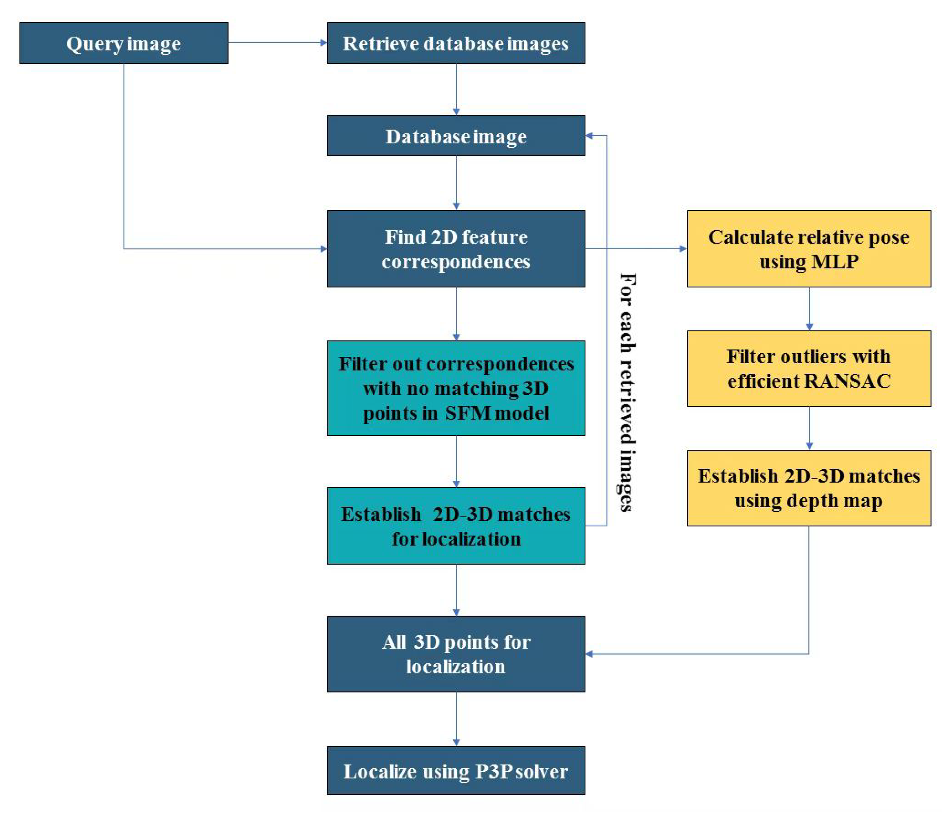
Figure 1. Illustration of different localization methods. Dark blue and cyan flow shows the general hierarchical localization pipeline, and dark blue and yellow flow shows the DLALoc pipeline.
Applsci 13 01076 g001
Figure 2. Mesh-based scene representation. (a,b) are two different views of the mesh-model.
Applsci 13 01076 g002
Figure 3. Form of five-point problem.
Applsci 13 01076 g003
Figure 4. The structure of learning-based algorithm.
Applsci 13 01076 g004
Figure 5. Two different SFM model. (a) sparse SFM model. (b) Original SFM model.
Applsci 13 01076 g005
Figure 6. Filtration effect of DLALoc method, from (ae) are the correctly retrieved database images, and DLAloc can efficiently filter out the outliers. (f) is the wrong retrieved database image, and DLALoc can filter out all mismatches.
Applsci 13 01076 g006aApplsci 13 01076 g006b
Figure 7. Comparison of localization accuracy and time with different anchor numbers.
Applsci 13 01076 g007
Table 1. Comparison of success rate tracked by MLP.
RoborCar Seasons/Aachen [%]Numbe of anchors
RANSAC Sampling Times4080120160200
51.5/4.84.7/7.28.5/16.48.9/17.68.8/17.9
103.5/6.96.1/11.312.5/21.712.9/22.313.5/24.3
305.1/7.95.4/13.213.7/25.412.8/23.213.3/24.6
505.7/6.26.9/14.714.8/28.914.5/22.515.2/24.8
1006.1/9.57.3/15.115.7/29.115.6/23.415.5/21.9
Table 2. Localization results of hierarchical localization baseline.
Hierarchical Localization Baseline
AachenRobotCar
DayNightDuskSunNight
Distance [m]0.25/0.50/5.00.5/1.0/5.00.25/0.50/5.00.25/0.50/5.00.25/0.50/5.0
Orient. [deg]2/5/102/5/102/5/102/5/102/5/10
NV+SIFT+NN82.6/87.3/92.934.2/46.8/60.156.7/83.5/94.946.1/67.8/91.05.1/10.9/23.9
NV+SIFT+SG84.6/88.7/93.754.5/71.7/86.963.2/87.9/95.461.1/74.9/93.57.2/18.4/33.6
NV+SP+NN83.7/88.4/93.240.8/56.4/73.759.2/86.7/95.158.5/69.7/93.36.7/17.3/31.1
NV+SP+SG88.0/94.9/97.870.2/87.4/98.467.9/88.9/96.957.4/67.8/92.66.4/18.1/30.9
HF-Net+NN75.7/88.3/90.145.9/61.1/78.955.6/85.6/95.246.7/74.6/95.93.2/6.9/17.7
HF-Net+SG87.6/92.4/93.765.4/85.9/94.464.8/87.1/95.846.3/67.4/90.94.7/17.5/24.9
Table 3. Localization results of DLALoc with 100 anchors and 25 RANSAC sampling times.
DLALoc with 100 Anchors and 25 RANSAC Sampling Times
AachenRobotCar
DayNightDuskSunNight
Distance [m]0.25/0.50/5.00.5/1.0/5.00.25/0.50/5.00.25/0.50/5.00.25/0.50/5.0
Orient. [deg]2/5/102/5/102/5/102/5/102/5/10
NV+SIFT+NN81.9/87.1/93.234.4/47.1/63.156.3/84.5/94.945.9/68.1/92.45.0/10.6/24.7
NV+SIFT+SG83.8/87.6/94.554.3/72.5/88.161.2/86.2/95.360.9/73.8/94.17.4/18.6/36.6
NV+SP+NN82.9/88.1/93.941.1/57.3/75.258.9/85.9/96.158.1/70.2/93.16.9/18.4/32.9
NV+SP+SG78.6/95.1/97.770.4/87.4/98.665.4/88.4/95.855.9/68.8/93.76.8/18.8/31.3
HF-Net+NN75.6/87.9/91.146.2/62.9/79.655.4/86.5/95.646.9/74.7/95.93.6/7.1/18.5
HF-Net+SG87.4/93.2/94.564.4/84.2/94.164.5/87.2/96.245.9/67.2/91.04.6/18.5/26.9
Table 4. Localization results of DLALoc with 100 anchors and 50 RANSAC sampling times.
DLALoc with 100 Anchors and 50 RANSAC Sampling Times
AachenRobotCar
DayNightDuskSunNight
Distance [m]0.25/0.50/5.00.5/1.0/5.00.25/0.50/5.00.25/0.50/5.00.25/0.50/5.0
Orient. [deg]2/5/102/5/102/5/102/5/102/5/10
NV+SIFT+NN84.9/88.4/94.345.4/58.1/76.258.2/86.3/95.150.1/71.2/93.17.8/13.6/26.1
NV+SIFT+SG84.9/89.1/95.657.6/74.8/89.963.4/88.9/96.264.1/75.6/94.88.5/20.3/37.9
NV+SP+NN84.7/89.6/93.942.6/58.9/76.960.1/87.1/96.459.8/72.8/93.97.5/19.6/34.2
NV+SP+SG78.9/95.4/97.974.6/89.6.4/98.868.4/88.9/96.957.2/69.9/94.57.9/19.6/32.4
HF-Net+NN74.6/90.9/94.555.6/68.9/93.858.4/89.5/96.449.3/77.9/96.94.5/8.6/20.4
HF-Net+SG88.6/94.4/95.666.1/87.2/96.657.8/89.4/96.747.1/68.9/92.45.0/19.6/27.5
Table 5. Localization results of DLALoc with 100 anchors and 100 RANSAC sampling times.
DLALoc with 100 Anchors and 100 RANSAC Sampling Times
AachenRobotCar
DayNightDuskSunNight
Distance [m]0.25/0.50/5.00.5/1.0/5.00.25/0.50/5.00.25/0.50/5.00.25/0.50/5.0
Orient. [deg]2/5/102/5/102/5/102/5/102/5/10
NV+SIFT+NN85.1/88.6/94.745.6/58.2/76.458.4/87.2/95.351.2/72.3/93.08.2/14.2/27.4
NV+SIFT+SG84.9/89.7/95.857.7/75.2/90.163.6/88.4/96.665.0/75.4/94.98.9/21.4/38.1
NV+SP+NN86.7/89.9/94.242.8/59.4/77.660.5/86.8/96.360.3/73.6/94.27.9/20.4/35.1
NV+SP+SG79.0/95.7/98.274.4/89.6/98.769.2/89.3/97.257.5/70.3/94.98.6/19.7/34.1
HF-Net+NN74.6/91.5/94.856.6/69.3/94.260.6/89.9/96.951.2/78.4/97.24.7/9.3/21.5
HF-Net+SG89.3/94.8/95.367.5/87.7/97.758.7/89.9/97.247.1/68.9/92.45.9/20.3/28.4
Table 6. Time and number of P3P points comparison of DLALoc with baseline methods.
Matching Time (min)P3P Time (min)MLP Time (min)Total Time (min)ImprovementLocal FeaturesP3P Points
NV+SP+NN6435.6-35.6-24922096
DLALoc(NV+SP+NN)6450.55.584.5%2492746
NV+SP+SG25820.4-20.4-17641657
DLALoc(NV+SP+SG)2584.10.54.676.7%17641032
HF-Net+NN6125.6-25.6-14321324
DLALoc(HF-Net+NN)614.30.54.881.3%1432998
Disclaimer/Publisher’s Note: The statements, opinions and data contained in all publications are solely those of the individual author(s) and contributor(s) and not of MDPI and/or the editor(s). MDPI and/or the editor(s) disclaim responsibility for any injury to people or property resulting from any ideas, methods, instructions or products referred to in the content.